Your script works. You tested it on the sample export — 1,000 rows — and it finished before your finger left the Enter key. You ship it. On Monday it runs against the real export: 1,000,000 rows. It is still running on Tuesday.
Nothing broke. There is no exception, no traceback, no bug in the ordinary sense. Every line does exactly what it did on Friday. The only thing that changed is how much data, and that is the one thing your code never mentioned.
# The Friday version. On 1,000 rows: 11 milliseconds. Ship it.
duplicates = []
for i in range(len(rows)):
    for j in range(i + 1, len(rows)):
        if rows[i] == rows[j] and rows[i] not in duplicates:
            duplicates.append(rows[i])
1,000× more data, and — measured later in this lesson, not guessed — roughly 1,000,000× more work. Three hours instead of eleven milliseconds. The fix is four lines long and finishes in 114 milliseconds.
Seeing Monday from Friday is the whole skill. It has a name — algorithmic thinking — and it is not about memorising sorting algorithms. It is about one question you learn to ask before you write the loop: what happens to this when the data gets big?
Why this matters
Here is the thing nobody tells beginners: your laptop is fast enough to hide your mistakes. A modern CPU does billions of operations a second, so at n=1,000 almost any algorithm finishes instantly. A linear scan, a nested loop, a bubble sort — all “fast.” Your test data is a liar. It tells you every approach works, right up until the day it doesn’t.
The gap does not creep up on you gradually. It detonates. Below is the same task — find the duplicate values in a list — written two ways, both measured on this machine with timeit. The only difference is the algorithm.
| Rows (n) | Two nested loops | A set, one pass | You’d notice? |
|---|---|---|---|
| 1,000 | 11.0 ms | 0.032 ms | No — both feel instant |
| 2,000 | 44.4 ms | 0.080 ms | No |
| 4,000 | 172.8 ms | 0.160 ms | Barely |
| 8,000 | 685.5 ms | 0.386 ms | The slow one blinks |
| 100,000 | ~1.8 minutes | 5.7 ms | Coffee |
| 1,000,000 | ~3 hours | 114 ms | You kill it and blame Python |
Read that table twice. At n=1,000 the two versions are separated by a rounding error, and every instinct you have says “don’t optimise prematurely, they’re both fine.” At n=1,000,000 one of them answers before you can blink and the other one is a Jira ticket. The choice you made when the data was small is the choice that decides what happens when it is big — and you cannot un-make it later without a rewrite.
Notice what the fast column is not: it is not the same algorithm written cleverly. There is no micro-optimisation here, no C extension, no multiprocessing, no rewriting it in Rust. It is the same Python, on the same machine, doing the same job — with a different shape. That shape is what Big-O measures, and it is the only performance idea in this lesson that will still be true in twenty years, on hardware that doesn’t exist yet.
The mental model to carry: Big-O is not a speed. It is a growth rate. It does not tell you how long your code takes; it tells you what happens to that time when your data gets ten times bigger. A fast O(n²) algorithm and a slow O(n) algorithm will cross — always — and Big-O tells you they will cross without you having to run anything. That is why we care about it even though we are about to measure everything: measurement tells you about today’s data, and Big-O tells you about next year’s.
Big-O: growth, not a stopwatch
Big-O notation describes how the work an algorithm does grows as its input grows. We write it O(something), where the “something” is a function of n — the size of the input. O(n) means “the work grows in proportion to n”: double the data, double the work. O(n²) means “double the data, quadruple the work.” That’s it. That’s the whole notation.
Three conventions make it useful, and each one looks like cheating until you see why.
We drop the constants. An algorithm that does 3n operations and one that does n operations are both O(n). This feels wrong — surely 3× slower matters? — but the constant depends on your CPU, your Python version, whether the data is in cache, and how you spell the loop. It is real, and it is not the interesting part, because it never changes the shape of the curve. A 3× penalty is a 3× penalty forever. An O(n²) algorithm’s penalty grows without limit. Constants are a fight you can win with better hardware; growth rates are not.
We drop the lower-order terms. 3n² + 5n + 200 is just O(n²), because as n grows the n² term drowns everything else. Not “approximately” — arithmetically:
| n | 3n² + 5n + 200 |
Just 3n² |
The n² term is… |
|---|---|---|---|
| 10 | 550 | 300 | 54.55% of the total |
| 100 | 30,700 | 30,000 | 97.72% |
| 1,000 | 3,005,200 | 3,000,000 | 99.83% |
| 1,000,000 | 3,000,005,000,200 | 3,000,000,000,000 | 100.00% |
By n=1,000 the +5n + 200 you were worried about accounts for 0.17% of the runtime. Keeping it in the notation would be false precision. The biggest term wins, and at scale it wins so completely that nothing else is worth writing down.
We usually mean the worst case. More on that shortly.
The ladder
There are six growth rates you will meet in practice. Learn them as a ladder, best at the top — and make it visceral straight away with the operation count at each size, plus how long that takes at a very optimistic 1 billion operations per second:
| Class | Name | You get it from | n=10 | n=1,000 | n=1,000,000 | Time @ n=1M |
|---|---|---|---|---|---|---|
| O(1) | Constant | Dict/set lookup, xs[i], len(), .append() |
1 | 1 | 1 | 1 ns |
| O(log n) | Logarithmic | Binary search, bisect, balanced trees |
3 | 10 | 20 | 20 ns |
| O(n) | Linear | A for loop, sum(), in on a list, max() |
10 | 1,000 | 1,000,000 | 1 ms |
| O(n log n) | Linearithmic | sorted(), .sort(), good general sorts |
33 | 9,966 | 19,931,569 | 20 ms |
| O(n²) | Quadratic | Nested loops, bubble sort, all-pairs | 100 | 1,000,000 | 1,000,000,000,000 | 16.7 min |
| O(2ⁿ) | Exponential | Naive recursion, brute-force subsets | 1,024 | 1.07 × 10³⁰¹ | overflow | longer than the universe |
Sit with the bottom two rows. At n=10, O(n²) costs 100 operations and O(2ⁿ) costs 1,024 — both instant, both apparently fine, and O(2ⁿ) is only 10× worse. At n=1,000, O(n²) needs a million operations (about a millisecond — still fine!) and O(2ⁿ) needs a number with 302 digits. For scale: there are roughly 10⁸⁰ atoms in the observable universe. The n=10 column is why you cannot test your way to this knowledge. Every row looks fine at n=10. That column is your sample data.
The O(n²) row is the one that will actually bite you, precisely because it is not absurd. It is plausible. It passes review. It ships. Sixteen minutes at n=1M is slow but not obviously insane — it’s the shape that makes n=10M take 28 hours.
And the top rows are why this lesson has a happy ending: O(1) is a flat line. Not “fast” — flat. It costs the same at n=1,000,000 as at n=10. In Python that flat line has a name, and you already know it: it’s a dict, and it’s a set.
The diagram below is that entire ladder, made real. It’s one task on one million rows, priced five ways, with every number measured by timeit on CPython 3.12 later in this lesson. Read it left → right and watch the cost climb: a hashed lookup answers in 15 nanoseconds; binary search needs 20 steps and 1.25 microseconds; a linear scan touches all million rows in 20.5 milliseconds; a full sort costs 136 milliseconds; and the two nested loops at the right-hand end take about three hours. Each arrow carries the real multiplier between its neighbours.
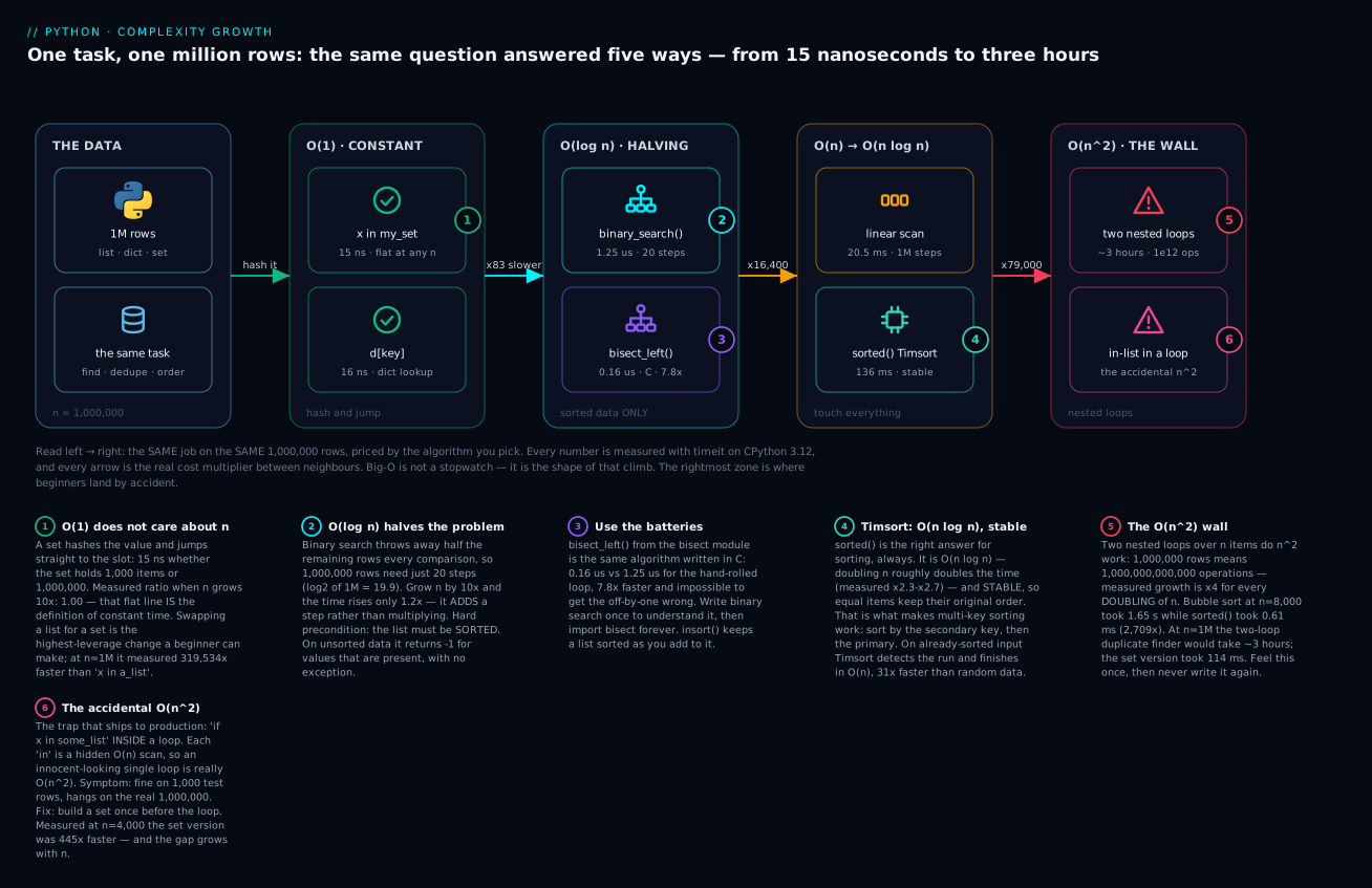
The badges mark the six things worth carrying out of this lesson: O(1) is genuinely flat, measuring the same 15 ns at every n (1); O(log n) halves the problem so a million rows cost 20 steps — but only on sorted data (2); bisect is that same algorithm in C, 7.8× faster and impossible to get wrong (3); sorted() is O(n log n) and stable, which is what makes multi-key sorting work (4); the O(n²) wall is where two nested loops put you (5); and the accidental O(n²) — x in a_list inside a loop — is the one that ships to production (6).
Reading a snippet’s complexity
You do not need mathematics for this. You need two rules and the willingness to count loops — so if for, while and nesting aren’t yet second nature, Control Flow: Conditionals, Loops & Logical Operators is the prerequisite for everything below.
Rule 1 — sequential steps ADD, and addition means the biggest one wins. Do an O(n) thing, then another O(n) thing? That’s O(n) + O(n) = O(2n) = O(n). Do an O(n) thing and then an O(n²) thing? O(n + n²) = O(n²). One after another, the worst step is your answer.
Rule 2 — nested steps MULTIPLY. A loop inside a loop, each running n times, does n × n = O(n²) work. This is the rule that matters, because nesting is how quadratic sneaks in.
# O(n) — one pass, n steps.
for row in rows:
    print(row)

# O(n) — two passes in sequence: n + n = 2n. Constants dropped -> O(n).
for row in rows:
    validate(row)
for row in rows:
    save(row)

# O(n^2) — a loop inside a loop: n * n.
for a in rows:
    for b in rows:
        compare(a, b)

# O(n^2) STILL — the inner loop averages n/2 iterations, giving n^2/2.
# Constants dropped. Half of catastrophic is catastrophic.
for i in range(len(rows)):
    for j in range(i + 1, len(rows)):
        compare(rows[i], rows[j])

# O(n log n) — an O(log n) operation done n times.
for row in rows:
    binary_search(sorted_index, row)

# O(1) — no loop over n at all. 1,000 iterations is a CONSTANT, not n.
for _ in range(1000):
    do_something()
That last one catches people. n is the thing that grows. A loop that always runs exactly 1,000 times is O(1) with an embarrassing constant, because it does not get slower when your data does. Meanwhile a loop that runs len(rows) times is O(n) even if rows currently has three items in it.
Now the rule that catches everyone, because the loop is invisible:
# Looks like ONE loop. Is actually O(n * m) — and O(n^2) when the lists are similar sizes.
for row in rows:                 # n iterations...
    if row.id in known_ids:      # ...and THIS is an O(m) scan if known_ids is a LIST
        matched.append(row)
There is no second for on the screen, so it reads as O(n). But in on a list is a hidden linear scan. Python is looping; you just aren’t. Every built-in that touches a collection has a cost, and if you don’t know it, you cannot read your own code. That is why the operations table further down is the single most valuable table in this lesson.
| Pattern | Complexity | Why |
|---|---|---|
for x in xs: |
O(n) | One pass over n items |
Two for loops in sequence |
O(n) | n + n = 2n; constants dropped |
for inside a for (both over n) |
O(n²) | Nested → multiply |
for i... for j in range(i+1, n) |
O(n²) | n²/2 pairs; constants dropped |
| Loop over n calling an O(log n) function | O(n log n) | Multiply n by log n |
| Loop over n calling an O(n) function | O(n²) | The call is the inner loop |
if x in a_list: inside a loop |
O(n²) | in on a list is a hidden O(n) scan |
if x in a_set: inside a loop |
O(n) | in on a set is O(1) — no hidden loop |
xs.sort() inside a loop |
O(n² log n) | Sorting n items, n times. Sort once, outside |
for _ in range(1000): |
O(1) | 1,000 is a constant — it doesn’t grow with n |
Halving each step (lo/hi window) |
O(log n) | 20 halvings gets you from 1M to 1 |
| Recursion branching twice per call | O(2ⁿ) | Each level doubles the calls |
Best, average, and worst case
An algorithm doesn’t have one running time — it has a range, depending on the data it gets. Linear search finds a match on the first comparison if you’re lucky and does all n comparisons if you’re not.
- Best case — the luckiest input. Mostly useless for decisions. Every algorithm is fast on its favourite input.
- Average case — a typical input. What you’ll actually experience.
- Worst case — the unluckiest input. This is what Big-O usually means, and it’s what you engineer for, because “usually fast” is no comfort at 3 a.m. when the input is adversarial or just unlucky.
| Algorithm | Best | Average | Worst | The worst case happens when… |
|---|---|---|---|---|
| Linear search | O(1) | O(n) | O(n) | The target is last, or absent |
| Binary search | O(1) | O(log n) | O(log n) | The target is a leaf of the search tree, or absent |
| Bubble sort | O(n) | O(n²) | O(n²) | Data is reverse-sorted (best case needs the early-exit swap flag) |
| Insertion sort | O(n) | O(n²) | O(n²) | Reverse-sorted; best case is already-sorted data |
Timsort (sorted()) |
O(n) | O(n log n) | O(n log n) | Genuinely random data; best case is sorted or reverse-sorted runs |
| Dict/set lookup | O(1) | O(1) | O(n) | Every key collides — vanishingly rare, but not impossible |
| Naive Fibonacci | O(2ⁿ) | O(2ⁿ) | O(2ⁿ) | Always. It has no good case |
Two rows there deserve a flag. Timsort’s O(n) best case is not a trivia item — it is the reason sorted() on already-sorted data measured 31× faster than on random data at n=1M in my benchmarks (4.4 ms vs 136 ms). Real data is often partly ordered, and Timsort was built to notice.
And dict lookup’s O(n) worst case is why we say “O(1) average.” With adversarial keys engineered to collide, a dict degrades to a linked list. In practice this never happens to you by accident; it’s a denial-of-service concern for web servers, which is why Python randomises string hashing per process by default.
Space complexity
Time is not the only cost. Space complexity is the same idea for memory: how much extra memory does the algorithm need as n grows? (By convention we don’t count the input itself — just what the algorithm allocates on top.)
| Approach | Space | Why it matters |
|---|---|---|
xs.sort() |
O(1)-ish | Sorts in place; Timsort needs a small temp buffer |
sorted(xs) |
O(n) | Builds a whole new list — at n=1M that’s another 8 MB |
| Binary search (iterative) | O(1) | Two integers, lo and hi |
| Binary search (recursive) | O(log n) | One stack frame per halving |
The seen = set() refactor |
O(n) | You trade memory for time — that’s the deal |
[x for x in huge] |
O(n) | Materialises everything |
(x for x in huge) |
O(1) | A generator — one item at a time |
| Naive recursive Fibonacci | O(n) stack | Depth n; RecursionError past ~1000 |
The seen = set() row is the honest bargain at the heart of this lesson. The O(n²) → O(n) refactor is not free — you pay for it in memory. You build a set holding up to n items to avoid scanning n items repeatedly. At n=1,000,000 that’s tens of megabytes to turn three hours into a tenth of a second — take that deal every time. But know you’re taking it: on a 500-million-row dataset that doesn’t fit in RAM, the calculation changes and you reach for a database or a chunked pass instead.
Searching: linear vs binary
Linear search: the honest baseline
Look at each item until you find it or run out. That’s it. It works on anything — sorted, unsorted, mixed, whatever — and it costs O(n).
def linear_search(items, target):
    """Return the index of target, or -1 if absent. Works on ANY list."""
    for i, item in enumerate(items):
        if item == target:
            return i
    return -1

data = [42, 7, 19, 3, 88, 1, 56]
print(linear_search(data, 88))     # => 4
print(linear_search(data, 99))     # => -1
In real Python you’d write 88 in data or data.index(88) — both are linear search implemented in C, and both are O(n). Writing the loop out is worth doing once so you can see the cost: the for loop is the O(n).
Binary search: throw away half, every time
If the data is sorted, you can do enormously better. Look at the middle. Too big? The answer is in the left half — throw the right half away. Too small? Throw the left half away. Repeat.
Each comparison eliminates half of everything that’s left. That’s the definition of O(log n), and log₂(1,000,000) ≈ 20, which is where the diagram’s “20 steps” comes from.
def binary_search(items, target):
    """Return the index of target, or -1. REQUIRES items to be sorted."""
    lo, hi = 0, len(items) - 1          # the window: inclusive on BOTH ends
    while lo <= hi:                     # <= : a 1-item window is still valid
        mid = (lo + hi) // 2
        if items[mid] == target:
            return mid
        if items[mid] < target:
            lo = mid + 1                # target is in the RIGHT half; mid is ruled out
        else:
            hi = mid - 1                # target is in the LEFT half; mid is ruled out
    return -1                           # lo passed hi -> the window is empty
Four details in those nine lines are where every bug lives, so name them out loud:
hi = len(items) - 1, notlen(items). The window is inclusive at both ends, sohiis a valid index. Uselen(items)and you’ll index off the end →IndexError.while lo <= hi, not<. Whenlo == hithere’s exactly one item left and it might be your answer. Use<and you’ll miss it — silently. (I measured this: onlist(range(10)), the<version reports 0, 3, 6 and 9 as missing.)mid + 1andmid - 1, notmid. You just checkedmid; it isn’t the answer, so exclude it. Writelo = midand when the window shrinks to two items it stops shrinking — an infinite loop.return -1after the loop.lo > himeans the window is empty and the value isn’t there.
Watch it work. Searching for 987 in list(range(1000)), printing the window at each step:
step  1: window [   0,  999] width 1000  mid= 499  items[mid]= 499
step  2: window [ 500,  999] width  500  mid= 749  items[mid]= 749
step  3: window [ 750,  999] width  250  mid= 874  items[mid]= 874
step  4: window [ 875,  999] width  125  mid= 937  items[mid]= 937
step  5: window [ 938,  999] width   62  mid= 968  items[mid]= 968
step  6: window [ 969,  999] width   31  mid= 984  items[mid]= 984
step  7: window [ 985,  999] width   15  mid= 992  items[mid]= 992
step  8: window [ 985,  991] width    7  mid= 988  items[mid]= 988
step  9: window [ 985,  987] width    3  mid= 986  items[mid]= 986
step 10: window [ 987,  987] width    1  mid= 987  items[mid]= 987
found at index 987 in 10 steps
The width column is the algorithm: 1000 → 500 → 250 → 125 → 62 → 31 → 15 → 7 → 3 → 1. Ten halvings and a thousand candidates became one. Linear search would have taken 988 comparisons to reach the same index.
The sorted precondition is not a suggestion
This is the part that matters most, and it is the reason binary search is dangerous in a way linear search never is. On unsorted data, binary search does not raise. It lies.
unsorted = [42, 7, 19, 3, 88, 1, 56]
print(binary_search(unsorted, 42))    # => -1   ...but 42 is at index 0
print(binary_search(unsorted, 7))     # => -1   ...but 7 is at index 1
print(binary_search(unsorted, 88))    # => -1   ...but 88 is at index 4
No TypeError. No ValueError. No warning. It returns “not found” for values sitting right there in the list, because it reasoned about halves of a list that was never ordered. A wrong answer delivered confidently is worse than a crash — a crash you fix on Tuesday; this you discover in a customer report in March.
The same trap applies to bisect. On that seven-item unsorted list, bisect-based lookup got six of the seven wrong — and the seventh right by pure luck. If your list came from a database, an API, a file, or anywhere you didn’t sort yourself, sort it or don’t binary search it.
The measured race
Now stop trusting me and look at the numbers. Same target (the last element — worst case for linear), timeit, best of three, CPython 3.12:
| n | Linear | Growth | Binary | Growth | Speedup |
|---|---|---|---|---|---|
| 10,000 | 202.9 µs | — | 0.89 µs | — | 228× |
| 100,000 | 2,049.6 µs | ×10.1 | 1.08 µs | ×1.2 | 1,901× |
| 1,000,000 | 20,510.4 µs | ×10.0 | 1.25 µs | ×1.2 | 16,356× |
Those growth columns are the whole point of this lesson. Forget the absolute numbers — they’re specific to this laptop and will be wrong on yours. Look at what happens when n goes up 10×:
- Linear search: ×10.0. Ten times the data, ten times the work. That is what O(n) looks like in a measurement. It’s not an approximation of the theory; it’s the theory’s fingerprint.
- Binary search: ×1.2. Ten times the data and it got 20% slower, because log₂ went from 17 to 20 — it added three comparisons while linear search added 900,000.
And the speedup column grows: 228× → 1,901× → 16,356×. A single benchmark number would have told you none of this. If I’d only measured n=10,000 and reported “binary search is 228× faster,” you’d have learned a fact about one dataset. The ratio across n tells you the shape, and the shape is what predicts n=100,000,000.
bisect: the batteries-included version
You now understand binary search, so you should almost never write it again. The standard library’s bisect module has it, in C, correct, since forever.
from bisect import bisect_left, bisect_right, insort

def bisect_search(items, target):
    """Binary search using the stdlib. items MUST be sorted."""
    i = bisect_left(items, target)
    if i != len(items) and items[i] == target:
        return i
    return -1

data = list(range(1_000_000))
print(bisect_search(data, 987_654))    # => 987654
bisect_left doesn’t return “found/not found” — it returns the insertion point: the index where target should go to keep the list sorted. That’s more useful than it sounds (it’s how you do range queries and nearest-neighbour lookups), but it means you must confirm the hit yourself with the items[i] == target check. Skip that check and you’ll “find” values that aren’t there.
Measured at n=1,000,000: hand-written binary search 1.25 µs, bisect_search 0.161 µs — 7.8× faster, same O(log n), zero chance of an off-by-one.
| Function | Returns | Use it for |
|---|---|---|
bisect_left(a, x) |
Insertion point, before any equal items | Finding the first occurrence of x |
bisect_right(a, x) / bisect(a, x) |
Insertion point, after any equal items | Finding where x ends; counting duplicates |
insort_left(a, x) / insort(a, x) |
None |
Inserting while keeping the list sorted |
bisect_left(a, x, lo, hi) |
Insertion point within a slice | Searching part of a list without copying it |
bisect_left(a, x, key=f) |
Insertion point by computed key | Searching a list of records (Python 3.10+) |
⚠️ One honest warning about insort: the search is O(log n) but the insert is O(n), because a list has to shift every later element. Building a sorted list by insort in a loop is O(n²) — slower than appending everything and calling sorted() once at the end. Use insort to maintain an already-sorted list you’re occasionally adding to, not to build one from scratch.
| Linear search | Binary search | |
|---|---|---|
| Precondition | None | Data must be sorted |
| Time | O(n) | O(log n) |
| Steps at n=1,000,000 | 1,000,000 | 20 |
| Measured at n=1M | 20,510 µs | 1.25 µs |
| On unsorted data | Correct | Silently wrong |
| Wins when | Data is unsorted, or you search once | Data is sorted and you search repeatedly |
| Python built-in | x in xs, xs.index(x) |
bisect.bisect_left |
That last row is the real decision. Sorting costs O(n log n) — more than a single linear scan. If you search a list once, sorting it first to binary search is a net loss. Sorting pays for itself when you search many times: pay O(n log n) once, then each of your k lookups costs O(log n) instead of O(n). And if you’re doing that, ask the question the next section answers: should this be a dict instead?
Sorting: feel O(n²) once, then never again
We’re going to implement bubble sort. Then we’re going to race it against sorted(), watch it lose by a factor of 2,709, and never speak of it again. The point is not that you’ll ever use it — you won’t, and you shouldn’t — the point is to feel a quadratic curve with your own hands so you recognise its shape for the rest of your career.
Bubble sort
Walk the list comparing neighbours; swap them if they’re out of order. Each pass “bubbles” the largest remaining item to the end. Repeat n times.
def bubble_sort(items):
    a = list(items)                     # copy: don't mutate the caller's list
    n = len(a)
    for i in range(n):                  # outer: n passes
        swapped = False
        for j in range(n - 1 - i):      # inner: the tail is already sorted
            if a[j] > a[j + 1]:
                a[j], a[j + 1] = a[j + 1], a[j]
                swapped = True
        if not swapped:                 # nothing moved -> already sorted -> stop
            break
    return a

print(bubble_sort([82, 15, 4, 95, 36, 32, 29, 18, 95, 14]))
# => [4, 14, 15, 18, 29, 32, 36, 82, 95, 95]
A loop inside a loop, both over n. That’s O(n²) — by Rule 2, nothing else to work out. The swapped flag buys a genuine O(n) best case (one clean pass over sorted data proves there’s nothing to do — measured at n=2,000: 0.062 ms on sorted input vs 98.9 ms on random, a 1,599× difference), but the average and worst cases are firmly quadratic.
Insertion sort
The other O(n²) sort worth seeing, because it’s what your hands do with playing cards: take each item and slide it back into its place among the already-sorted items on its left.
def insertion_sort(items):
    a = list(items)
    for i in range(1, len(a)):
        key = a[i]
        j = i - 1
        while j >= 0 and a[j] > key:    # slide bigger items right
            a[j + 1] = a[j]
            j -= 1
        a[j + 1] = key                  # drop key into the gap
    return a
Same O(n²), but with a much better constant — measured a consistent 2.4× faster than bubble sort at every n from 250 to 4,000. It’s also stable and adaptive (nearly-sorted data is nearly O(n)), which is why insertion sort is genuinely useful — Timsort itself uses it on small chunks. This is a good moment to notice that “same Big-O” does not mean “same speed”: constants are real, they just don’t change the shape. And the 2.4× stays 2.4× as n grows — a constant factor, not a diverging curve.
| Algorithm | Best | Average | Worst | Stable? | Measured at n=4,000 |
|---|---|---|---|---|---|
| Bubble sort | O(n) | O(n²) | O(n²) | Yes | 405.4 ms |
| Insertion sort | O(n) | O(n²) | O(n²) | Yes | 166.1 ms |
Timsort (sorted()) |
O(n) | O(n log n) | O(n log n) | Yes | 0.27 ms |
The race
timeit, best of three, random floats, CPython 3.12:
| n | Bubble | Growth | sorted() |
Growth | sorted() wins by |
|---|---|---|---|---|---|
| 1,000 | 22.4 ms | — | 0.038 ms | — | 585× |
| 2,000 | 96.9 ms | ×4.32 | 0.105 ms | ×2.74 | 921× |
| 4,000 | 405.4 ms | ×4.19 | 0.267 ms | ×2.54 | 1,520× |
| 8,000 | 1,653.0 ms | ×4.08 | 0.610 ms | ×2.29 | 2,709× |
There it is: double n, quadruple the time. ×4.32, ×4.19, ×4.08 — that is O(n²) signing its name. Meanwhile sorted() grows ×2.29–×2.74 per doubling: a bit more than double, because that’s n log n — the n doubles and the log n creeps up by one.
And the final column is why the growth ratio matters more than any single benchmark. sorted() isn’t “about a thousand times faster than bubble sort” — that’s not a fact, it’s a snapshot. It’s 585× faster at n=1,000 and 2,709× faster at n=8,000, and the gap widens forever, because the two functions are on different curves. Extrapolate that ×4 curve out to n=1,000,000 and bubble sort needs roughly seven hours. sorted() measured 136 milliseconds.
sorted() and .sort()
Python’s sort is Timsort — invented by Tim Peters for CPython in 2002, and since adopted by Java, Android, V8, Swift and Rust. It’s a hybrid: it finds naturally-ordered runs in your data, extends short ones with insertion sort, and merges them. It’s O(n log n) guaranteed, stable, and adaptive.
That “adaptive” is not marketing. Real-world data is rarely random — it’s log lines that arrive mostly in time order, records that came out of a database with an ORDER BY, a list that was sorted and then had ten items appended. Timsort spots those runs:
| Input at n=1,000,000 | Measured | vs random |
|---|---|---|
| Already sorted | 4.4 ms | 31× faster |
| Reverse sorted | 4.5 ms | 30× faster |
| Random floats | 136.4 ms | baseline |
Reverse-sorted being just as fast surprises people: Timsort finds descending runs too, and simply reverses them in place. Both cases hit the O(n) best case.
The two spellings are not interchangeable, and the difference is the single most common beginner bug in Python:
xs.sort() |
sorted(xs) |
|
|---|---|---|
| Kind | List method | Built-in function |
| Works on | Lists only | Any iterable — tuple, set, dict, str, generator |
| Returns | None |
A new list, always |
| Original | Modified in place | Untouched |
| Extra memory | O(1)-ish | O(n) — a whole new list |
| Use when | You own the list and want it sorted | You need a sorted copy, or the input isn’t a list |
names = ["zoe", "adam", "kim"]
result = names.sort()
print(result)          # => None                      <- NOT the sorted list!
print(names)           # => ['adam', 'kim', 'zoe']    <- the sort DID happen, in place

first = names.sort()[0]
Traceback (most recent call last):
  File "<stdin>", line 1, in <module>
    first = names.sort()[0]
            ~~~~~~~~~~~~^^^
TypeError: 'NoneType' object is not subscriptable
.sort() returns None because it has nothing to hand back — it changed names itself. Python’s convention is deliberate and consistent: methods that mutate in place return None, precisely so you can’t mistake a mutation for a copy. 'NoneType' object is not subscriptable is that lesson arriving late. (Full treatment of list methods and this trap lives in Lists & Tuples: Indexing, Slicing, Methods & Immutability.)
And sorting mixed types fails, because Python refuses to invent an order:
TypeError: '<' not supported between instances of 'str' and 'int'
key= and the decorate-sort pattern
key takes a function, calls it once per item, and sorts by the results. This is the workhorse.
words = ["banana", "Fig", "apple", "cherry"]

print(sorted(words))                 # => ['Fig', 'apple', 'banana', 'cherry']
# 'Fig' first: capital letters have lower codepoints than lowercase.
print(sorted(words, key=str.lower))  # => ['apple', 'banana', 'cherry', 'Fig']
print(sorted(words, key=len))        # => ['Fig', 'apple', 'banana', 'cherry']

rows = [("web02", "prod", 3), ("db01", "dev", 1), ("web01", "prod", 3)]
print(sorted(rows, key=lambda r: r[2]))            # by tier
print(sorted(rows, key=lambda r: (r[2], r[0])))    # by tier, then host — TUPLE key
print(sorted(rows, key=lambda r: -r[2]))           # numeric descending
key is called exactly n times, not once per comparison. I verified this: sorting 1,000 items called the key function exactly 1,000 times, though it made ~10,000 comparisons. Python decorates each item with its key up front, sorts the decorated pairs, then throws the keys away. That’s the decorate–sort–undecorate pattern (the “Schwartzian transform”), and it used to be something you wrote by hand:
# The old manual way — this is what key= does for you now.
decorated = sorted((w.lower(), i, w) for i, w in enumerate(words))
result = [w for _, _, w in decorated]
print(result)                        # => ['apple', 'banana', 'cherry', 'Fig']
print(sorted(words, key=str.lower))  # => ['apple', 'banana', 'cherry', 'Fig']  same
The i in the middle is the historical reason it’s worth knowing: it breaks ties before Python ever compares the third element, so two equal keys never cause a TypeError on uncomparable objects. key= handles all of this — but when you see this pattern in old code, now you know what it is.
⚠️ The anti-pattern to avoid: functools.cmp_to_key() wraps an old-style comparison function, which gets called once per comparison instead of once per item. Measured: 8,613 calls for n=1,000, versus 1,000 for a key. It exists for porting Python 2 code. Reach for a key (or a tuple key) instead.
Stability, and why it’s the feature you didn’t know you needed
Stable means: items that compare equal keep their original relative order. Timsort guarantees this. It sounds academic. It is the thing that makes multi-key sorting work at all.
rows = [("web02", "prod", 3), ("db01", "dev", 1), ("web01", "prod", 3),
        ("api1", "dev", 1), ("cache", "prod", 1)]

# Sort by tier, then by host name within each tier.
# The trick: sort by the SECONDARY key first, then the PRIMARY.
step1 = sorted(rows, key=lambda r: r[0])       # secondary: host
step2 = sorted(step1, key=lambda r: r[2])      # primary: tier
print([(r[0], r[2]) for r in step2])
# => [('api1', 1), ('cache', 1), ('db01', 1), ('web01', 3), ('web02', 3)]

# Single pass with a tuple key — same result, and what you should normally write.
one = sorted(rows, key=lambda r: (r[2], r[0]))
print([(r[0], r[2]) for r in one])
# => [('api1', 1), ('cache', 1), ('db01', 1), ('web01', 3), ('web02', 3)]
print(step2 == one)                            # => True
The two-pass version only works because the second sort is stable: when it reorders by tier, it doesn’t disturb the host ordering the first sort established. On an unstable sort, pass two would scramble pass one and you’d get garbage.
Use the tuple key when you can — one pass, obviously correct. But the two-pass trick is the escape hatch for the case a tuple key can’t express: different directions on non-numeric keys. You can negate a number (-r[2]) to flip it inside a tuple; you cannot negate a string.
# tier ASCENDING, host name DESCENDING — impossible in one tuple key.
result = sorted(sorted(rows, key=lambda r: r[0], reverse=True),
                key=lambda r: r[2])
print([(r[0], r[2]) for r in result])
# => [('db01', 1), ('cache', 1), ('api1', 1), ('web02', 3), ('web01', 3)]
One more subtlety that catches experienced people: reverse=True is not the same as reversed(sorted(...)). reverse=True preserves stability; reversing the output flips the ties too.
pairs = [(1, "a"), (2, "b"), (1, "c"), (2, "d")]
print(sorted(pairs, key=lambda p: p[0], reverse=True))
# => [(2, 'b'), (2, 'd'), (1, 'a'), (1, 'c')]     ties still in original order
print(list(reversed(sorted(pairs, key=lambda p: p[0]))))
# => [(2, 'd'), (2, 'b'), (1, 'c'), (1, 'a')]     ties REVERSED too
Here is every sorting recipe in one place — the table to keep open in a second tab:
| Goal | Spelling | Note |
|---|---|---|
| Case-insensitive | key=str.lower |
Bare method, no lambda needed |
| By length | key=len |
|
| By a field | key=lambda r: r[2] |
key=itemgetter(2) measured 1.69× faster |
| By an attribute | key=attrgetter("price") |
Both from the operator module |
| By a computed value | key=lambda r: r[1] * r[2] |
Sort by something not in the data |
| Multi-key, all ascending | key=lambda r: (r[2], r[0]) |
Tuple key — one pass, preferred |
| Multi-key, numeric descending | key=lambda r: (-r[2], r[0]) |
Negate the number — you can’t negate a string |
| Mixed directions, non-numeric | sorted(sorted(rows, key=b, reverse=True), key=a) |
Two passes, secondary first — relies on stability |
| Descending, ties preserved | sorted(rows, key=f, reverse=True) |
Almost always what you want |
| Descending, ties flipped | reversed(sorted(rows, key=f)) |
Almost never what you want |
If key=lambda ... and higher-order functions feel unfamiliar, Lambda & Higher-Order Functions covers exactly why passing a function as an argument works.
The Pythonic punchline: pick the right data structure
Everything so far has been about algorithms. Now the plot twist, and the most valuable idea in this lesson:
In Python, choosing the right data structure usually beats writing a clever algorithm.
You will almost never hand-write a sort. You will constantly choose between a list, a dict, and a set — and that choice routinely swings performance by five orders of magnitude. It is not a micro-optimisation. It’s a different curve.
The measurement that should change how you write Python
in on a list is O(n) — Python scans until it finds a match. in on a set or dict hashes the value and jumps straight to the slot: O(1). Worst-case membership (the last element), timeit, CPython 3.12:
| n | x in list |
Growth | x in set |
Growth | Set is |
|---|---|---|---|---|---|
| 1,000 | 4.50 µs | — | 0.0148 µs | — | 304× faster |
| 10,000 | 44.98 µs | ×9.99 | 0.0148 µs | ×1.00 | 3,034× |
| 100,000 | 462.89 µs | ×10.29 | 0.0148 µs | ×1.00 | 31,240× |
| 1,000,000 | 4,725.63 µs | ×10.21 | 0.0148 µs | ×1.00 | 319,534× |
Look at that set column. 0.0148 µs. 0.0148 µs. 0.0148 µs. 0.0148 µs. A thousand items or a million items — identical. Growth ratio 1.00. This is not “fast.” Fast is a list at n=1,000. This is flat, and flat is a different thing entirely: it means the size of your data has stopped being your problem.
That’s what O(1) means, and it’s why the last column climbs to 319,534×. The set didn’t get faster. The list got slower, and the set didn’t care.
The refactor: two loops → a hash map
This is the pattern. It’s the most common real interview question, and more importantly it’s the most common real production fix. You’ll recognise it now from the opening of this lesson:
# BEFORE — O(n^2). Two loops, plus 'not in dupes' is itself a hidden O(n) scan.
def find_duplicates_slow(items):
    dupes = []
    for i in range(len(items)):
        for j in range(i + 1, len(items)):
            if items[i] == items[j] and items[i] not in dupes:
                dupes.append(items[i])
    return dupes

# AFTER — O(n). One pass. A set answers "have I seen this?" in constant time.
def find_duplicates_fast(items):
    seen = set()
    dupes = set()
    for item in items:
        if item in seen:
            dupes.add(item)
        else:
            seen.add(item)
    return list(dupes)
Measured:
| n | Two loops | Growth | Set | Growth | Speedup |
|---|---|---|---|---|---|
| 1,000 | 11.0 ms | — | 0.032 ms | — | 339× |
| 2,000 | 44.4 ms | ×4.06 | 0.080 ms | ×2.46 | 559× |
| 4,000 | 172.8 ms | ×3.89 | 0.160 ms | ×2.01 | 1,082× |
| 8,000 | 685.5 ms | ×3.97 | 0.386 ms | ×2.42 | 1,774× |
| 1,000,000 | ~3 hours (extrapolated) | — | 114 ms | — | ~95,000× |
×4 per doubling versus ×2 per doubling. Quadratic versus linear, in the measurement, exactly as the theory promised.
The recognition rule, which is worth more than the code: whenever you see a loop inside a loop asking “does this thing over here match that thing over there?”, you are looking at an O(n²) that wants to be an O(n). Replace the inner loop with a set or dict built once, outside. The same refactor is the answer to two-sum, to “find the intersection,” to “which records are missing,” to “group these by key” — it’s one pattern wearing different hats.
The generalisation: a nested loop searching for something is a hash lookup that hasn’t been written yet.
The accidental O(n²)
You don’t have to write two for loops to get quadratic. You just have to put an in on a list inside a loop:
# Looks linear. Is quadratic. This is the one that ships.
matched = [x for x in a if x in b]        # b is a LIST -> each 'in' scans it
| n (both lists) | b is a list |
b is a set |
Speedup |
|---|---|---|---|
| 1,000 | 1.664 ms | 0.0149 ms | 112× |
| 2,000 | 6.650 ms | 0.0307 ms | 217× |
| 4,000 | 26.841 ms | 0.0603 ms | 445× |
Note the list column quadrupling per doubling — the O(n²) fingerprint — while the set column doubles. The fix is one word: b = set(b) before the loop. That single line converts an O(n²) into an O(n).
Watch for the same shape in .index() inside a loop, if x in df["col"].values, list.remove() in a loop, and if key in list_of_keys. All the same bug. All the same fix. The dict and set behaviour behind this — hashing, why keys must be immutable — is covered in Dictionaries & Sets: Key/Value & Membership.
The complexity of Python’s own operations
This is the table to bookmark. You cannot reason about your code’s complexity without knowing what the built-ins cost. Times measured at n=1,000,000, CPython 3.12:
| Operation | Complexity | Measured @ n=1M | Note |
|---|---|---|---|
xs[i] (get/set) |
O(1) | 7.6 ns | Contiguous array — pure arithmetic |
len(xs) |
O(1) | 18.9 ns | Stored, not counted |
xs.append(v) |
O(1) amortised | 9.5 ns | Over-allocates; occasional resize |
xs.pop() (end) |
O(1) | 15.1 ns | Nothing shifts |
xs.insert(0, v) |
O(n) | 4.7 µs | Every element shifts right |
xs.pop(0) |
O(n) | 147.1 µs | Every element shifts left |
x in xs (list) |
O(n) | 4.92 ms | Linear scan — the big one |
xs.index(x) |
O(n) | 5.01 ms | Same scan |
xs.sort() / sorted(xs) |
O(n log n) | 136 ms | Timsort; O(n) on sorted input |
xs[a:b] (slice) |
O(k) | — | Copies k references |
d[key] (dict get) |
O(1) avg | 16.0 ns | Hash and jump |
d[key] = v (dict set) |
O(1) avg | 18.6 ns | |
key in d (dict) |
O(1) avg | 15.9 ns | |
x in s (set) |
O(1) avg | 15.1 ns | 326,000× faster than the list |
s.add(x) |
O(1) avg | 14.2 ns | |
deque.appendleft(x) |
O(1) | 13.4 ns | 351× faster than list.insert(0) |
deque.popleft() |
O(1) | 16.3 ns | 9,000× faster than list.pop(0) |
"".join(parts) |
O(n) | — | The right way to build a string |
s += x in a loop |
O(n)* | — | *CPython-only optimisation — see below |
Three rows are worth internalising above all others. x in xs on a list at n=1M costs 4.92 milliseconds — 326,000× more than the same question asked of a set. xs.pop(0) costs 147 µs versus 15 ns for pop() — if you’re using a list as a queue, you want collections.deque. And append is 9.5 ns — Python’s most common operation is essentially free, which is why “build a list then convert” beats almost every clever alternative.
An honest detour: measuring beats guessing
Every Python performance guide tells you that building a string with += in a loop is O(n²), because strings are immutable so each += copies the whole string. I was going to tell you that. Then I measured it:
| n | s += "x" in a loop |
Growth |
|---|---|---|
| 10,000 | 0.400 ms | — |
| 20,000 | 0.798 ms | ×2.00 |
| 40,000 | 1.597 ms | ×2.00 |
| 80,000 | 3.288 ms | ×2.06 |
×2.00 per doubling. That’s linear. The folklore is wrong — or rather, it’s wrong on CPython specifically, because CPython contains an optimisation: when a string’s reference count is exactly 1, += can resize the buffer in place instead of copying. In the loop above, s is the only reference, so the optimisation fires every time.
So the folklore is nonsense? No — watch what happens when I hold one extra reference and defeat it:
| n | keep = s; s += "x" |
Growth |
|---|---|---|
| 10,000 | 1.118 ms | — |
| 20,000 | 3.465 ms | ×3.10 |
| 40,000 | 12.059 ms | ×3.48 |
| 80,000 | 96.576 ms | ×8.01 |
The quadratic comes roaring back — at n=100,000 it measured 48× slower than the optimised form. One extra reference, and the curve changes shape.
Three lessons, and they’re the reason this section exists:
- Measure, don’t recite. I would have shipped a plausible, widely-repeated claim that my own machine disproves in four lines.
- A single number would have hidden this. Only the growth ratio across n reveals it — ×2.00 versus ×3.10→×8.01.
- Use
"".join()anyway. It measured 0.34 ms at n=100,000 versus 4.05 ms for the optimised+=— 12× faster — and it’s O(n) unconditionally, not because of a fragile refcount detail that any refactor, any other Python implementation (PyPy, Jython), or one stray reference can silently turn back into a quadratic.
That’s the mature version of “premature optimisation is the root of all evil.” The point was never don’t think about performance. It’s don’t guess. Get the shape right up front — that’s free, it’s just knowing which data structure to reach for — and measure before you tune anything else.
Measuring honestly with timeit
time.perf_counter() around one call is not a measurement, it’s an anecdote. Your OS scheduled another process; the CPU changed frequency; the first run paid for a cache miss the second didn’t. timeit exists to handle this: it runs your code many times and reports the best run — because noise only ever makes things slower, so the minimum is the closest thing to the truth.
import timeit

# stmt and setup as strings — setup is NOT timed.
t = timeit.timeit("999_999 in data",
                  setup="data = set(range(1_000_000))",
                  number=100_000)
print(f"{t / 100_000 * 1e9:.1f} ns per lookup")     # => 15.1 ns per lookup
The trap that invalidates most beginner benchmarks — timing your setup:
# WRONG — this measures building a 100,000-item list 100 times.
timeit.timeit("data = list(range(100_000)); 99_999 in data", number=100)
# => 1508.6 us per call

# RIGHT — setup runs once and is not timed.
timeit.timeit("99_999 in data", setup="data = list(range(100_000))", number=100)
# => 467.8 us per call
69% of the “measurement” was building the list. Anything you learned from the first number was about list(range(...)), not about in.
The harness I used for every table in this lesson, which handles the “how many repeats?” problem for you:
import timeit

def measure(func, *args):
    """Best-of-3 seconds per call to func(*args)."""
    timer = timeit.Timer(lambda: func(*args))
    number, _ = timer.autorange()    # auto-picks a loop count so the total is >= 0.2s
    return min(timer.repeat(repeat=3, number=number)) / number
Timer.autorange() is the underrated part: it scales the loop count to the function. Measured on my machine it chose 200,000 loops for a microsecond-scale function and 50 for a millisecond-scale one — automatically, so a fast function gets enough iterations to beat the clock’s resolution and a slow one doesn’t take all afternoon.
| Tool | Use | Gotcha |
|---|---|---|
timeit.timeit(stmt, setup, number=N) |
Quick one-off | Returns total time for N runs — divide it yourself |
timeit.repeat(stmt, setup, repeat=5, number=N) |
Better | Take min(), not mean — noise is one-sided |
timeit.Timer(callable) |
Time a function object | Wrap args in a lambda |
Timer.autorange() |
Auto loop count | Targets ≥ 0.2 s total |
python3 -m timeit -s "setup" "stmt" |
From the shell | Best for a fast comparison |
time.perf_counter() |
One slow operation | Noise-dominated below ~10 ms |
cProfile |
Which function is slow | Adds overhead; use for shape, not absolutes |
%timeit |
Jupyter/IPython | Same engine, nicer output |
The methodology rule this lesson lives by: never measure at one n. One number tells you about one dataset on one machine. Measure at n, 2n, 4n — the ratio is the Big-O signature, it’s portable across machines, and it’s the thing that predicts what happens on data you haven’t seen yet.
Patterns worth knowing
Four patterns cover a startling fraction of real code and coding interviews. Each is a way of turning an O(n²) into an O(n) or O(n log n).
Two-pointer — walk a sorted list from both ends. Each step rules out one candidate, so it’s O(n) instead of the O(n²) of checking all pairs.
def two_sum_sorted(nums, target):
    lo, hi = 0, len(nums) - 1
    while lo < hi:
        s = nums[lo] + nums[hi]
        if s == target:
            return (lo, hi)
        if s < target:
            lo += 1          # need a BIGGER sum -> raise the low end
        else:
            hi -= 1          # need a SMALLER sum -> lower the high end
    return None

prices = [12, 25, 30, 47, 58, 61, 79]
print(two_sum_sorted(prices, 88))     # => (2, 4)      30 + 58 = 88
print(two_sum_sorted(prices, 1000))   # => None
Hash map (the two-sum) — the same problem without the sorted precondition, in one pass. This is the single most-asked coding interview question, and it’s the refactor from the last section wearing a different hat.
def two_sum(nums, target):
    seen = {}                        # value -> index
    for i, n in enumerate(nums):
        want = target - n
        if want in seen:             # O(1) -- have I already passed my partner?
            return (seen[want], i)
        seen[n] = i
    return None

nums = [47, 12, 79, 25, 61, 30, 58]
print(two_sum(nums, 88))             # => (5, 6)      30 + 58 = 88
The insight worth stealing: instead of asking “is there a partner somewhere ahead?” (which forces an inner loop), it asks “did my partner already go past?” — which a dict answers in O(1). Measured against the nested-loop version: ×4.00 growth per doubling versus ×2.00, and 1,216× faster at n=4,000.
Sliding window — a contiguous run over a list where you add the new item and subtract the old one instead of re-summing. Turns O(n·k) into O(n).
def max_window_sum(nums, k):
    if len(nums) < k:
        return None
    window = sum(nums[:k])
    best = window
    for i in range(k, len(nums)):
        window += nums[i] - nums[i - k]     # add the new, drop the old -> O(1) per step
        best = max(best, window)
    return best

reqs = [3, 1, 4, 1, 5, 9, 2, 6, 5, 3]
print(max_window_sum(reqs, 3))              # => 17      9 + 2 + 6
Counting with a dict — the answer to “how many of each?”, “most common”, “are these anagrams?”, “is there a duplicate?”.
from collections import Counter

words = "the quick brown fox jumps over the lazy dog the fox".split()

counts = {}
for w in words:
    counts[w] = counts.get(w, 0) + 1        # .get(w, 0) avoids a KeyError
print(counts["the"], counts["fox"])         # => 3 2

print(Counter(words).most_common(2))        # => [('the', 3), ('fox', 2)]
| Pattern | Turns | Into | Precondition | Classic question |
|---|---|---|---|---|
| Two-pointer | O(n²) | O(n) | Sorted | Pair with a given sum; remove duplicates in place |
| Hash map | O(n²) | O(n) | Hashable items | Two-sum; find duplicates; intersection |
| Sliding window | O(n·k) | O(n) | Contiguous run | Max sum of k; longest substring without repeats |
| Counting dict | O(n²) | O(n) | Hashable items | Most common; anagrams; first unique character |
| Sort first | O(n²) | O(n log n) | Comparable | Group duplicates; find the median; merge intervals |
The last row is the fallback worth remembering: when you can’t hash it, sort it. Sorting costs O(n log n) but it puts equal things next to each other, which collapses a lot of pair-comparison problems into one linear pass. Hash if you can, sort if you can’t, nested-loop never.
Hands-on lab
Everything here is pure standard library — nothing to install. (For the habit: python3 -m venv .venv && source .venv/bin/activate, or .venv\Scripts\activate on Windows, where the command is python rather than python3.)
python3 --version
# Python 3.12.3
Create algo_lab.py and add each step to the bottom, running python3 algo_lab.py as you go. The whole lab runs in about 40 seconds. Every output below is real output from this machine — your absolute timings will differ, and that’s fine. The growth ratios are the point, and those should match.
Start the file with the imports:
import math
import random
import timeit
from bisect import bisect_left
Step 1 — Build an honest measuring harness.
def measure(func, *args):
    """Best-of-3 seconds per call to func(*args)."""
    timer = timeit.Timer(lambda: func(*args))
    number, _ = timer.autorange()
    return min(timer.repeat(repeat=3, number=number)) / number
What just happened: autorange() picks a loop count so each timing runs for at least 0.2 s — enough iterations that clock resolution stops mattering. min() of three repeats because noise only ever slows things down. Every number in this lab comes from this function, so the comparisons are apples to apples.
Step 2 — Implement both searches, and prove they agree.
def linear_search(items, target):
    for i, item in enumerate(items):
        if item == target:
            return i
    return -1

def binary_search(items, target):
    lo, hi = 0, len(items) - 1
    while lo <= hi:
        mid = (lo + hi) // 2
        if items[mid] == target:
            return mid
        if items[mid] < target:
            lo = mid + 1
        else:
            hi = mid - 1
    return -1

data = list(range(1000))
print(linear_search(data, 987), binary_search(data, 987))
print(linear_search(data, 5000), binary_search(data, 5000))
assert all(linear_search(data, x) == binary_search(data, x) for x in range(-5, 1005))
print("agree on all 1010 probes")
987 987
-1 -1
agree on all 1010 probes
What just happened: before timing anything, you proved both functions are correct — on every value present, absent, and past both ends. A fast wrong answer is worthless. (That assert is a real test: change <= to < in binary_search and it fires immediately.)
Step 3 — Count comparisons, not seconds.
def linear_steps(items, target):
    steps = 0
    for item in items:
        steps += 1
        if item == target:
            return steps
    return steps

def binary_steps(items, target):
    lo, hi, steps = 0, len(items) - 1, 0
    while lo <= hi:
        steps += 1
        mid = (lo + hi) // 2
        if items[mid] == target:
            return steps
        if items[mid] < target:
            lo = mid + 1
        else:
            hi = mid - 1
    return steps

print(f"{'n':>10} | {'linear':>9} | {'binary':>6} | {'log2(n)':>7}")
print("-" * 42)
for n in (10, 1_000, 100_000, 1_000_000):
    d = list(range(n))
    print(f"{n:>10,} | {linear_steps(d, n-1):>9,} | {binary_steps(d, n-1):>6} | {math.log2(n):>7.1f}")
         n |    linear | binary | log2(n)
------------------------------------------
        10 |        10 |      4 |     3.3
     1,000 |     1,000 |     10 |    10.0
   100,000 |   100,000 |     17 |    16.6
 1,000,000 | 1,000,000 |     20 |    19.9
What just happened: Big-O made concrete with zero timing involved. The binary column tracks log2(n) exactly — that’s not a coincidence, it’s the definition. A million rows in 20 comparisons.
Step 4 — Race them, and watch the growth ratio.
print(f"{'n':>10} | {'linear':>10} | {'growth':>6} | {'binary':>8} | {'growth':>6} | {'speedup':>8}")
print("-" * 66)
pl = pb = None
for n in (10_000, 100_000, 1_000_000):
    d = list(range(n))
    tl = measure(linear_search, d, n - 1)
    tb = measure(binary_search, d, n - 1)
    gl = f"x{tl/pl:.1f}" if pl else "-"
    gb = f"x{tb/pb:.1f}" if pb else "-"
    pl, pb = tl, tb
    print(f"{n:>10,} | {tl*1e6:>7.1f} us | {gl:>6} | {tb*1e6:>5.2f} us | {gb:>6} | {tl/tb:>7,.0f}x")
         n |     linear | growth |   binary | growth |  speedup
------------------------------------------------------------------
    10,000 |   202.9 us |      - |  0.89 us |      - |     228x
   100,000 |  2049.6 us |  x10.1 |  1.08 us |  x1.2 |   1,901x
 1,000,000 | 20510.4 us |  x10.0 |  1.25 us |  x1.2 |  16,356x
What just happened: the growth columns are the Big-O, measured. 10× the data → ×10.0 for linear (that is O(n)) and ×1.2 for binary (that is O(log n): it added three comparisons while linear added 900,000). The speedup climbing 228× → 16,356× is the two curves diverging in real time.
Step 5 — Use the batteries.
def bisect_search(items, target):
    i = bisect_left(items, target)
    if i != len(items) and items[i] == target:
        return i
    return -1

d = list(range(1_000_000))
print(bisect_search(d, 987_654))
t_hand = measure(binary_search, d, 999_999)
t_bis = measure(bisect_search, d, 999_999)
print(f"hand-written {t_hand*1e6:.2f} us | bisect {t_bis*1e6:.3f} us | "
      f"bisect is {t_hand/t_bis:.1f}x faster")
987654
hand-written 1.25 us | bisect 0.161 us | bisect is 7.8x faster
What just happened: the same O(log n), written in C. Same shape, better constant, and no chance of an off-by-one. Write binary search once to understand it; import bisect forever.
Step 6 — Break the precondition on purpose.
unsorted = [42, 7, 19, 3, 88, 1, 56]
for t in (42, 7, 88):
    print(f"binary_search(unsorted, {t:>2}) = {binary_search(unsorted, t):>3}  "
          f"but {t} IS at index {unsorted.index(t)}")
binary_search(unsorted, 42) =  -1  but 42 IS at index 0
binary_search(unsorted,  7) =  -1  but 7 IS at index 1
binary_search(unsorted, 88) =  -1  but 88 IS at index 4
What just happened: no exception — just wrong answers. This is the most important failure in the lab. Binary search cannot detect unsorted input; it trusts you. Every “not found” here is a lie, and in a real system it would be a silent data bug, not a crash.
Step 7 — Feel O(n²) with your own hands.
def bubble_sort(items):
    a = list(items)
    n = len(a)
    for i in range(n):
        swapped = False
        for j in range(n - 1 - i):
            if a[j] > a[j + 1]:
                a[j], a[j + 1] = a[j + 1], a[j]
                swapped = True
        if not swapped:
            break
    return a

random.seed(42)
small = [random.randint(1, 99) for _ in range(10)]
print(small)
print(bubble_sort(small))
print(bubble_sort(small) == sorted(small))
print()
print(f"{'n':>7} | {'bubble':>10} | {'growth':>6} | {'sorted()':>9} | {'growth':>6} | {'ratio':>7}")
print("-" * 62)
pb = ps = None
for n in (1_000, 2_000, 4_000, 8_000):
    d = [random.random() for _ in range(n)]
    tb = measure(bubble_sort, d)
    ts = measure(sorted, d)
    gb = f"x{tb/pb:.2f}" if pb else "-"
    gs = f"x{ts/ps:.2f}" if ps else "-"
    pb, ps = tb, ts
    print(f"{n:>7,} | {tb*1e3:>7.1f} ms | {gb:>6} | {ts*1e3:>6.3f} ms | {gs:>6} | {tb/ts:>6,.0f}x")
[82, 15, 4, 95, 36, 32, 29, 18, 95, 14]
[4, 14, 15, 18, 29, 32, 36, 82, 95, 95]
True

      n |     bubble | growth |  sorted() | growth |   ratio
--------------------------------------------------------------
  1,000 |    22.4 ms |      - |  0.038 ms |      - |    585x
  2,000 |    96.9 ms |  x4.32 |  0.105 ms |  x2.74 |    921x
  4,000 |   405.4 ms |  x4.19 |  0.267 ms |  x2.54 |  1,520x
  8,000 |  1653.0 ms |  x4.08 |  0.610 ms |  x2.29 |  2,709x
⚠️ This step takes ~10 seconds — bubble sort at n=8,000 genuinely needs 1.65 s per call. That delay is the lesson. Don’t raise n much further unless you enjoy waiting: n=16,000 would take ~7 s per call.
What just happened: ×4 per doubling. That’s O(n²), measured. sorted() grows ×2.3–2.7 (that’s n log n), and the gap widens from 585× to 2,709× as n grows — because they’re on different curves and always will be. Bubble sort was also correct (== sorted(small) printed True); it’s not wrong, it’s quadratic, which at scale is worse than wrong.
Step 8 — The refactor that matters.
def find_duplicates_slow(items):
    dupes = []
    for i in range(len(items)):
        for j in range(i + 1, len(items)):
            if items[i] == items[j] and items[i] not in dupes:
                dupes.append(items[i])
    return dupes

def find_duplicates_fast(items):
    seen, dupes = set(), set()
    for item in items:
        if item in seen:
            dupes.add(item)
        else:
            seen.add(item)
    return list(dupes)

random.seed(42)
sample = [random.randint(1, 20) for _ in range(15)]
print(sample)
print(sorted(find_duplicates_slow(sample)), sorted(find_duplicates_fast(sample)))
print(sorted(find_duplicates_slow(sample)) == sorted(find_duplicates_fast(sample)))
print()
print(f"{'n':>7} | {'two loops':>10} | {'growth':>6} | {'set':>9} | {'growth':>6} | {'speedup':>8}")
print("-" * 64)
pa = pf = None
for n in (1_000, 2_000, 4_000, 8_000):
    d = [random.randint(0, n * 2) for _ in range(n)]
    ta = measure(find_duplicates_slow, d)
    tf = measure(find_duplicates_fast, d)
    ga = f"x{ta/pa:.2f}" if pa else "-"
    gf = f"x{tf/pf:.2f}" if pf else "-"
    pa, pf = ta, tf
    print(f"{n:>7,} | {ta*1e3:>7.1f} ms | {ga:>6} | {tf*1e3:>6.3f} ms | {gf:>6} | {ta/tf:>7,.0f}x")

n = 1_000_000
d = [random.randint(0, n * 2) for _ in range(n)]
t = measure(find_duplicates_fast, d)
print(f"\nset version at n=1,000,000: {t*1e3:.0f} ms")
print(f"two-loop at n=1,000,000 would be ~{(n/8_000)**2 * pa / 3600:,.1f} hours")
[4, 1, 9, 8, 8, 5, 4, 18, 3, 19, 14, 2, 1, 3, 7]
[1, 3, 4, 8] [1, 3, 4, 8]
True

      n |  two loops | growth |       set | growth |  speedup
----------------------------------------------------------------
  1,000 |    11.0 ms |      - |  0.032 ms |      - |     339x
  2,000 |    44.4 ms |  x4.06 |  0.080 ms |  x2.46 |     559x
  4,000 |   172.8 ms |  x3.89 |  0.160 ms |  x2.01 |   1,082x
  8,000 |   685.5 ms |  x3.97 |  0.386 ms |  x2.42 |   1,774x

set version at n=1,000,000: 114 ms
two-loop at n=1,000,000 would be ~3.0 hours
What just happened: the lesson’s opening story, closed. Both functions return the same answer — verified on line 3 — but one is ×4 per doubling and the other is ×2. At n=1,000,000 that’s three hours versus 114 milliseconds, and the last line extrapolates it from your own measured ×4 curve rather than asking you to take my word for it.
You’ve now, in eight steps: built an honest measuring harness; implemented and verified two searches; counted the comparisons that make O(log n) real; measured the growth ratios that are the Big-O signature; seen bisect beat your hand-written version 7.8×; watched binary search lie about unsorted data; felt a quadratic curve; and turned an O(n²) into an O(n) with a set.
Common mistakes and troubleshooting
| Symptom / traceback | Cause | Fix |
|---|---|---|
Binary search returns -1 for values that are in the list |
The list isn’t sorted. Binary search cannot detect this — it just reasons about halves that don’t exist | data.sort() first, or use linear search / in. No exception is raised — this is a silent data bug, so assert the precondition in dev |
IndexError: list index out of range in binary search |
hi = len(items) instead of len(items) - 1, so mid can point past the end |
The window is inclusive: hi = len(items) - 1 |
| Binary search misses items at window edges | while lo < hi instead of <= — a 1-item window is skipped |
Use while lo <= hi. Verified: on list(range(10)) the < version reports 0, 3, 6, 9 as missing |
| Binary search hangs forever | lo = mid instead of lo = mid + 1 — with 2 items left the window stops shrinking |
lo = mid + 1 / hi = mid - 1. You already checked mid; exclude it |
TypeError: 'NoneType' object is not subscriptable |
.sort() mutates in place and returns None; you used its return value |
sorted(xs) for a new list, or call xs.sort() on its own line then use xs |
TypeError: '<' not supported between instances of 'str' and 'int' |
Sorting mixed types — Python refuses to invent an order | Make the types uniform, or give a key: sorted(xs, key=str). Same error from sorted([1, None]) |
| Script is instant on test data, hangs on real data | An O(n²) that n=1,000 hid. Usually x in a_list inside a loop, or .index() in a loop |
Build a set/dict once before the loop. Measured 445× at n=4,000, and the gap grows |
| A “one loop” function is mysteriously quadratic | in, .index(), .remove(), .count() on a list are hidden O(n) scans |
Know the ops table. in on a set is O(1) — 326,000× faster at n=1M |
| Sorting inside a loop | xs.sort() per iteration = O(n² log n) |
Sort once, outside the loop |
RecursionError: maximum recursion depth exceeded |
Recursive binary search / deep recursion past sys.getrecursionlimit() (default 1000) |
Rewrite iteratively (this lesson’s binary_search is a while loop for exactly this reason). Raising the limit with setrecursionlimit risks a hard interpreter crash |
| Benchmark numbers make no sense / everything looks equally slow | timeit is measuring your setup — building the data inside the timed statement |
Move it to setup=. Measured: 69% of the “result” was list(range(100_000)) |
| Benchmark is noisy and unrepeatable | Single-shot time.perf_counter() on a sub-millisecond operation |
timeit with repeat, take min() — never mean. Use Timer.autorange() to pick the loop count |
| Optimised the wrong thing; nothing got faster | You tuned a function that wasn’t the bottleneck | Profile first (cProfile), fix the biggest term. A 2× win on 3% of runtime is a 1.5% win |
list.pop(0) / insert(0, x) in a loop crawls |
Both are O(n) — every element shifts | collections.deque: measured 9,000× faster for popleft() at n=1M |
bisect “finds” values that aren’t there |
bisect_left returns an insertion point, not a match |
Always confirm: i != len(a) and a[i] == target |
Building a sorted list with insort in a loop is slow |
The search is O(log n) but the insert is O(n) → O(n²) overall | append everything, then sorted() once |
Three of these deserve extra words, because they cost the most hours.
1. Binary search on unsorted data — the bug that doesn’t raise. Every other mistake in this table announces itself with a traceback. This one hands you a confident wrong answer. The failure mode is brutal in production: your data was sorted when you wrote the code, and eight months later someone adds a row in the wrong place, or changes the query’s ORDER BY, or feeds it a merged list — and lookups start returning “not found” for records that exist. Nothing crashes. Nothing logs. If you binary search a list you did not sort in the same function, either sort it there or add a real assertion (assert data == sorted(data) is O(n log n) and fine in a dev build — just don’t ship it in the hot path).
2. The accidental O(n²) — the bug that ships. Nobody writes two nested for loops over a million rows on purpose. What they write is:
for row in new_rows:              # n
    if row.id not in existing_ids:    # existing_ids is a LIST -> O(m) scan
        insert(row)
One visible loop. Reads as linear. Is quadratic, because in on a list is a loop you didn’t write. It passes review, passes tests (n=50 in the fixtures), and falls over in production. The fix is one word: existing_ids = set(existing_ids) before the loop. Train your eye to see in, .index(), .count() and .remove() on a list inside a loop as if a second for were printed there in red — because there is.
3. Optimising the wrong thing. “Premature optimisation is the root of all evil” gets quoted to shut down performance conversations, which inverts what Knuth meant. The real hierarchy: complexity is design, and everything else is tuning. Choosing a set over a list costs nothing — no extra code, no cleverness, no readability tax — and it’s the difference between 114 milliseconds and three hours. That’s not premature; that’s just knowing your tools. What is premature is rewriting a function in C, caching aggressively, or reaching for multiprocessing before you’ve profiled — especially when the real problem is an O(n²) that no amount of constant-factor tuning can rescue. Get the shape right for free, then measure, then tune what the profiler actually points at. A 100× constant-factor win on an O(n²) algorithm just moves the wall from n=8,000 to n=80,000.
Cheat-sheet
| Syntax / concept | What it does |
|---|---|
| O(1) | Constant — dict/set lookup, xs[i], len(), .append() |
| O(log n) | Halving — binary search, bisect. 1M rows → 20 steps |
| O(n) | One pass — for, sum(), x in a_list, max() |
| O(n log n) | Sorting — sorted(), .sort() |
| O(n²) | Nested loops — bubble sort, all-pairs comparison |
| O(2ⁿ) | Every subset — naive recursion. Hopeless past n≈40 |
| Loops nest → | Multiply the complexities |
| Loops in sequence → | Add → the biggest term wins |
| Drop constants & lower terms | 3n² + 5n + 200 → O(n²) |
| Growth ratio = the signature | n→2n: ×2 is O(n) · ×4 is O(n²) · ×2.3 is O(n log n) |
x in a_list |
O(n) — 4.92 ms at n=1M |
x in a_set / x in a_dict |
O(1) — 15 ns at any n |
d[key] / d[key] = v |
O(1) average |
xs[i] / xs.append(v) / len(xs) |
O(1) |
xs.insert(0, v) / xs.pop(0) |
O(n) — use collections.deque |
deque.appendleft() / .popleft() |
O(1) at both ends |
xs.index(v) / xs.remove(v) / xs.count(v) |
O(n) — hidden loops |
sorted(xs) |
New list, any iterable, O(n log n), O(n) memory |
xs.sort() |
In place, lists only, returns None |
| Timsort | O(n log n) worst, O(n) on sorted input, stable |
sorted(xs, key=f) |
f called once per item (decorate-sort-undecorate) |
sorted(xs, key=lambda r: (a, b)) |
Multi-key — tuple key, one pass |
sorted(xs, key=lambda r: (-n, s)) |
Numeric descending inside a tuple key |
sorted(sorted(xs, key=b, reverse=True), key=a) |
Mixed directions — secondary first, needs stability |
sorted(xs, key=f, reverse=True) |
Descending, ties preserved |
reversed(sorted(xs, key=f)) |
Descending, ties flipped — usually a bug |
key=itemgetter(1) |
1.69× faster than the equivalent lambda |
from bisect import bisect_left |
Binary search in C — 7.8× faster than hand-rolled |
bisect_left(a, x) |
Insertion point before equals — confirm a[i] == x! |
bisect_right(a, x) |
Insertion point after equals |
insort(a, x) |
Insert keeping sorted — search O(log n), insert O(n) |
| Binary search precondition | Data must be sorted — else silently wrong, no exception |
while lo <= hi / lo = mid + 1 / hi = mid - 1 |
The three lines every binary search bug lives in |
seen = set() refactor |
The O(n²) → O(n) move. Costs O(n) memory |
| Two-pointer | Sorted list, walk from both ends → O(n) |
| Sliding window | window += new - old → O(1) per step |
Counter(xs).most_common(k) |
Counting, in C |
timeit.repeat(stmt, setup, repeat=5, number=N) |
Take min(), never mean |
Timer.autorange() |
Auto-picks the loop count (targets ≥0.2 s) |
python3 -m timeit -s "setup" "stmt" |
Quick shell benchmark |
| Never measure at one n | Measure at n, 2n, 4n — the ratio is the Big-O |
sys.getrecursionlimit() |
1000 — why binary search should be iterative |
Interview and exam questions
Q: What is Big-O notation, and why do we drop constants?
A: It describes how work grows as the input grows — not how long the code takes. We drop constants because they depend on your CPU, Python version and cache behaviour, and they never change the shape of the curve: a 3× penalty is 3× forever, while an O(n²) penalty grows without limit. We drop lower-order terms because the biggest one dominates — in 3n² + 5n + 200 at n=1,000,000, the n² term is 100.00% of the total. Big-O is about the crossover that’s guaranteed to happen, not about today’s stopwatch.
Q: Give the complexity of x in a_list vs x in a_set, and explain the difference.
A: O(n) versus O(1) average. A list must scan item by item; a set hashes the value and jumps straight to the slot. Measured worst-case at n=1,000,000: 4,725 µs vs 0.0148 µs — 319,534× faster — and the set’s time is identical at n=1,000 (growth ratio 1.00), which is what O(1) actually means. The set’s worst case is technically O(n) if every key collides, which is why we say “O(1) average”; in practice it never happens by accident.
Q: How do you spot an O(n²) in code that only has one visible loop?
A: Look for a hidden linear operation inside the loop. if x in a_list, a_list.index(x), .count(), .remove(), sum() of a slice — each is an O(n) scan Python performs for you. One visible for × one hidden scan = O(n²). The tell is that it’s fast on test fixtures and hangs on production data. The fix is to hoist a set/dict out of the loop.
Q: When is binary search the wrong choice?
A: When the data isn’t sorted and you’ll only search once — sorting costs O(n log n), which is more than a single O(n) scan, so you’d lose. It also can’t work on unsorted data at all: it returns wrong answers silently, with no exception. And if you’re searching a lot and can hash the items, a set/dict is O(1), which beats O(log n) anyway. Binary search’s niche: sorted data (often because it’s sorted for another reason), searched repeatedly, where hashing isn’t available — e.g. range queries, or “find the nearest value below x.”
Q: What is Timsort, and why does stability matter?
A: Python’s sort: a hybrid of merge sort and insertion sort that finds naturally-ordered runs in the data. O(n log n) worst case, O(n) on already-sorted input (measured 31× faster at n=1M), and stable — equal items keep their original relative order. Stability is what makes multi-key sorting work: sort by the secondary key, then by the primary, and the second sort won’t disturb the first’s ordering. It’s also why reverse=True differs from reversed(sorted(...)): the former preserves tie order, the latter flips it.
Q: How would you sort records by tier ascending, then by hostname descending?
A: A tuple key can’t express mixed directions on a string — you can negate a number (key=lambda r: (-r.tier, r.host)) but not a string. So use the stability trick: sort by the secondary key first with its own direction, then by the primary. sorted(sorted(rows, key=lambda r: r.host, reverse=True), key=lambda r: r.tier). Two passes, still O(n log n), and correct only because Timsort is stable.
Q: .sort() vs sorted() — what’s the difference, and what does .sort() return?
A: .sort() is a list method that sorts in place and returns None; sorted() is a built-in that takes any iterable and returns a new list. .sort() returns None because Python’s convention is that mutating methods return None — a guard rail against mistaking a mutation for a copy. names.sort()[0] raises TypeError: 'NoneType' object is not subscriptable. .sort() uses O(1) extra memory; sorted() allocates a whole new list (another 8 MB for a million ints).
Q (coding): Given a list of integers, find whether any value appears twice. What’s your complexity? A: One pass with a set — O(n) time, O(n) space:
def has_duplicate(nums):
    seen = set()
    for n in nums:
        if n in seen:
            return True
        seen.add(n)
    return False
The naive two-loop version is O(n²) time, O(1) space. The set version trades memory for time — the right call almost always. If you can’t spare the memory, sorted(nums) then check adjacent pairs: O(n log n) time, O(1) extra space if you sort in place. Naming that trade-off out loud is what the interviewer is actually listening for.
Q (coding): Two-sum — return the indices of two numbers adding to a target. Better than O(n²)? A: One pass with a dict — O(n):
def two_sum(nums, target):
    seen = {}                      # value -> index
    for i, n in enumerate(nums):
        want = target - n
        if want in seen:
            return (seen[want], i)
        seen[n] = i
    return None
The insight: instead of asking “is my partner somewhere ahead?” (which needs an inner loop), ask “did my partner already go past?” — a dict answers that in O(1). If the input were sorted, the two-pointer approach gives O(n) with O(1) space instead.
Q: What does key= do, and how many times is it called?
A: It computes the value to sort by, and it’s called exactly once per item — not once per comparison. Verified: sorting 1,000 items calls it 1,000 times while making ~10,000 comparisons. Python decorates each item with its key, sorts the pairs, and discards the keys — the decorate-sort-undecorate pattern, built in. This is why key= is fast and why functools.cmp_to_key is slow (8,613 calls for the same 1,000 items, because it runs per comparison).
Q: You have an O(n²) function that’s fast enough today. Do you fix it? A: Ask what n is and whether it grows. If n is bounded and small (a config file’s 20 entries), O(n²) is fine and clarity wins. If n comes from user data, a database, or a file that grows, fix it now — it’s the same code length, so there’s no trade-off to weigh. This is where “premature optimisation” gets misquoted: complexity is a design decision, not an optimisation. Choosing a set over a list costs nothing and buys you three hours. Rewriting in C before profiling is the premature part — and a 100× constant win on an O(n²) just moves the wall from n=8,000 to n=80,000.
Q: How do you benchmark Python code honestly?
A: timeit, not a stopwatch — it runs the code many times and you take the min(), because noise is one-sided (it only ever slows things down; mean and stdev just measure your OS). Keep data construction in setup=, never in the timed statement — I measured a case where 69% of the “result” was building the list. And critically: measure at several n and report the ratio. A single number tells you about one dataset; ×2 per doubling is O(n) and ×4 is O(n²), and that ratio is portable to machines you’ll never touch. It also catches folklore — I “knew” that s += x in a loop was O(n²) until CPython’s in-place optimisation measured ×2.00 per doubling, and only holding a second reference brought the quadratic back.
Q: Why is list.pop(0) slow, and what should you use instead?
A: A list is a contiguous array of references, so removing the first item shifts every other element left — O(n). Measured at n=1M: pop() 15.1 ns vs pop(0) 147 µs, roughly 9,700× slower. Use collections.deque, which is O(1) at both ends (popleft() measured 16.3 ns). This is the standard “using a list as a queue” bug — and it’s a data-structure fix, not an algorithm fix, which is the theme of this whole lesson.
Key takeaways
- Big-O is a growth rate, not a stopwatch. It answers “what happens when the data gets 10× bigger?” Constants and lower-order terms are dropped because they never change the shape of the curve — at n=1M, the
n²in3n² + 5n + 200is 100.00% of the work. Your laptop is fast enough to hide every one of these mistakes at n=1,000. - The growth ratio is the real signature — so never measure at one n. Double n: ×2 is O(n), ×4 is O(n²), ×2.3 is O(n log n). A single benchmark describes one dataset on one machine; the ratio predicts data you haven’t seen. Measured here: linear search ×10.0 per 10× n, binary search ×1.2, bubble sort ×4.1 per doubling,
sorted()×2.3. - Read complexity by counting loops: nested multiply, sequential add. The hidden loops are what get you —
in,.index(),.count(),.remove()on a list are all O(n) scans, so one visibleforaround anif x in a_listis a quadratic in disguise. That’s the bug that passes review and dies in production. - Linear search works on anything and costs O(n). Binary search costs O(log n) — 20 steps for a million rows — but demands sorted data. Break that precondition and it doesn’t raise; it lies, returning “not found” for values that are present. Write it once to learn the
lo <= hi/mid ± 1details, then usebisectforever (measured 7.8× faster, in C, and impossible to get wrong). - Implement bubble sort once, feel the ×4-per-doubling, then never write it again.
sorted()is Timsort: O(n log n) worst case, O(n) on already-sorted input (31× faster at n=1M), and stable — which is exactly what makes multi-key sorting work. Remember.sort()returnsNone, use tuple keys for multi-key, and reach for the two-pass trick only when directions differ on non-numeric fields. - The Pythonic punchline: the right data structure beats the clever algorithm.
x in a_setmeasured 0.0148 µs at every n — growth ratio 1.00, 319,534× faster than a list at n=1M. The list got slower; the set never noticed. Most real performance work is alist→set/dict/dequeswap, not an algorithm. - “Two loops → hash map” is THE pattern. Whenever a nested loop asks “does this match that?”, a set or dict built once outside collapses O(n²) → O(n). Measured on the duplicate finder: three hours → 114 ms at n=1M. You pay for it in O(n) memory — take that deal, but know you’re taking it.
- Measure, don’t recite — and get the shape right for free.
timeitwithmin()of several repeats, data insetup=, several values of n. It’s how I caught myself about to repeat the folklore thats += xis O(n²) (CPython’s refcount-1 optimisation makes it linear — until one extra reference brings the quadratic back, 48× slower). Complexity is a design decision that costs nothing; everything after it is tuning that needs a profiler.