You have forty-five minutes, a shared editor with no autocomplete, and a stranger watching you type. The problem on the screen is one you’ve never seen. Your brain, helpfully, has gone completely blank.
This is the coding interview, and it terrifies good engineers who ship real software every day — because it does not look like the job. Nobody at work makes you invert a binary tree from memory while narrating your thoughts. So the myth grows: you have to grind 500 LeetCode problems. People do exactly that, burn out, and still freeze, because they were memorising answers instead of learning to recognise questions.
Here is the thing the grind hides. The thousands of problems are not a thousand different problems. They are about ten patterns wearing different costumes. “Two-sum,” “find the pair that adds to k,” “does any value repeat,” “group the anagrams” — four different prompts, one pattern: build a hash map, look things up in O(1). Once you can see the pattern under the costume, an unseen problem stops being a memory test and becomes a matching exercise: which of my ten tools does this clue point at?
# The prompt says "sorted" and "pair that sums to target."
# That single clue -> two-pointer. The code writes itself once you see it.
def two_sum_sorted(nums, target):
    lo, hi = 0, len(nums) - 1
    while lo < hi:
        s = nums[lo] + nums[hi]
        if s == target:
            return [lo, hi]
        if s < target:
            lo += 1          # sum too small -> raise the floor
        else:
            hi -= 1          # sum too big -> lower the ceiling
    return None

print(two_sum_sorted([2, 7, 11, 15], 9))    # => [0, 1]
This lesson teaches the ten patterns — each as clue → template → a worked example that actually runs — plus the interview process that is graded just as hard as the code: clarifying the problem, stating a brute-force solution before the clever one, getting the Big-O right, and testing your own edge cases. Every snippet here was executed on CPython 3.12; the outputs are real, and where a complexity claim can be measured, it is.
Why this matters
The coding interview is the gate to most software jobs above a certain level, and it is almost entirely learnable — which is the good news and the reason to take it seriously. It rewards preparation of a specific, unglamorous kind: not talent, not a maths degree, not raw problem-solving genius, but familiarity with a small set of patterns and enough calm to run a process under pressure.
The trap is treating it as a knowledge quiz with 500 answers to memorise. Memorised solutions are brittle: change one constraint — “now the array isn’t sorted,” “now find all pairs,” “now it’s a stream too big for memory” — and the memorised answer breaks, while you have no method to rebuild it. Pattern recognition is robust: you recognise the shape, adapt the template, and re-derive the details live. That’s the difference between a candidate who freezes when the problem is 10% different from the one they studied, and one who says “this is a sliding window with a twist” and just solves it.
There is a second thing beginners miss entirely: the interviewer is grading your process, not just your final answer. A candidate who clarifies the problem, talks through a brute-force approach, states its complexity, optimises it, and tests edge cases — but doesn’t quite finish the code — often passes, while a candidate who silently types a perfect memorised solution with no explanation can fail. The interviewer is simulating a work session: can you take an underspecified problem, reason about trade-offs out loud, and produce correct code you actually verified? That is the job. The algorithm is the medium, not the message.
This lesson assumes you can read Big-O — if “O(n²) vs O(n)” doesn’t yet make your stomach drop, do Algorithmic Thinking: Search, Sort & Big-O in Python first, because complexity is the language you’ll state answers in. Everything else we build from scratch.
How a coding interview actually works
A typical technical screen or on-site coding round runs 30–60 minutes on one or two problems. What is happening is not “can you produce the answer” — the interviewer usually knows the optimal solution cold and has seen it fifty times. What they’re assessing is closer to “would I want to debug production with this person at 2 a.m.?” Concretely, they are watching five things, and each is a place you can win or lose points independent of whether the code is perfect.
| What they watch | What a strong candidate does | What sinks you |
|---|---|---|
| Communication | Thinks out loud; narrates the approach before and while coding | Silent typing; the interviewer has no idea what you’re doing |
| Problem clarification | Restates the problem, asks about input size, empties, duplicates, sortedness | Assumes; solves the wrong problem fast |
| Approach & trade-offs | States brute force + its Big-O, then optimises, explaining the swap | Jumps to a memorised optimum with no reasoning (reads as memorised) |
| Correctness | Writes clean code, dry-runs one example, fixes bugs found | Hand-waves “and then it works”; never runs it mentally |
| Testing | Drives their own code through edge cases before being asked | “Looks right to me” — and the interviewer hands them the empty input |
Read that table as a scoring rubric, because it essentially is one. Notice that only one of the five rows is about the code being optimal. You can produce a merely-decent algorithm and still score well on the other four — and four out of five is usually a pass. Conversely, a beautiful O(n) solution typed in silence with no edge-case testing hits one row and misses four.
The single highest-leverage habit is thinking out loud. It feels unnatural — you don’t narrate your thoughts at your desk — but in an interview, silence is an information vacuum the interviewer fills with doubt. Talking does three things: it lets the interviewer help you (a good one will nudge you off a dead end, but only if they can hear where you are), it demonstrates the reasoning they’re actually grading, and it slows you down enough to catch your own mistakes. A candidate who says “I’ll use a hash map here to get O(1) lookups instead of scanning the list each time” has just scored on communication, approach, and complexity in one sentence — before writing any code.
The second habit: clarify before you code. The problem statement is deliberately underspecified, and the questions you ask are graded. “Can the array be empty?” “Are there duplicates?” “Is it already sorted?” “How big can n get — hundreds, or billions?” “Can values be negative?” These aren’t stalling; each answer changes the solution, and asking them proves you’ve been burned by unspecified requirements before — which is exactly the experience the interviewer is probing for. The candidate who codes for two minutes and then discovers the input can be empty has shown the opposite.
The questions aren’t random — they’re a checklist keyed to the input type, and each one has a concrete consequence for your code. Memorise the consequence, not just the question:
| Ask about | Concrete question | Why — what it changes |
|---|---|---|
| Size | “How large can n get?” | Decides whether O(n²) is acceptable at all, or you must hit O(n)/O(n log n) |
| Emptiness | “Can the input be empty or None?” |
The if not x: return ... guard that stops an IndexError/AttributeError |
| Duplicates | “Are values unique, or can they repeat?” | Set vs multiset; whether two-sum can pair an element with itself |
| Order | “Is the data sorted?” | Unlocks two pointers / binary search — or forces a hash map |
| Sign & range | “Negatives? Floats? Huge values?” | Sliding window breaks on negatives; sign affects prefix-sum logic |
| Output shape | “Return the index, the value, or a boolean? First match or all?” | Changes the whole return contract — and whether one pass suffices |
| Ties / multiple answers | “If several answers exist, any one, or a specific one?” | Whether you can early-return or must scan on |
Spend ninety seconds here and the pattern often reveals itself as a side effect — “it’s sorted and I want a pair” is the two-pointer recognition. Clarifying and matching are the same motion done well.
UMPIRE: a method you can run under pressure
When your mind goes blank, you don’t need inspiration — you need a checklist you can run mechanically until your brain reboots. Several exist (some call it “clarify–plan–code–test”); a memorable one is UMPIRE. The letters matter less than the discipline of always doing the steps in order, out loud, even when you think you know the answer.
| Step | Stands for | What you do | Why it scores |
|---|---|---|---|
| U | Understand | Restate the problem; ask clarifying questions; write down 2-3 examples | Proves you solve the right problem; surfaces edge cases early |
| M | Match | Which pattern do the clues point at? “Sorted?” “Contiguous?” “Count?” | This is the core skill — recognition, not recall |
| P | Plan | Describe the approach in words / pseudocode before typing real code | Interviewer can course-correct you cheaply, before you’ve written 30 lines |
| I | Implement | Write clean code, narrating as you go | The actual coding — now the easy part, because the thinking is done |
| R | Review | Dry-run one example line by line; check off-by-ones, empties | Catches bugs before the interviewer does; shows you don’t trust “looks right” |
| E | Evaluate | State time and space complexity; test edge cases; note improvements | Closes strong on the two rows candidates most often skip |
The diagram below is this method drawn as a left-to-right spine — the path a strong answer walks from reading the problem to a tested, complexity-stated solution. The two red zones are the ones worth tattooing on the inside of your eyelids: a wrong Big-O claim and skipped edge cases are how candidates who wrote correct code still walk out with a reject. Both are cheap to avoid and expensive to skip.
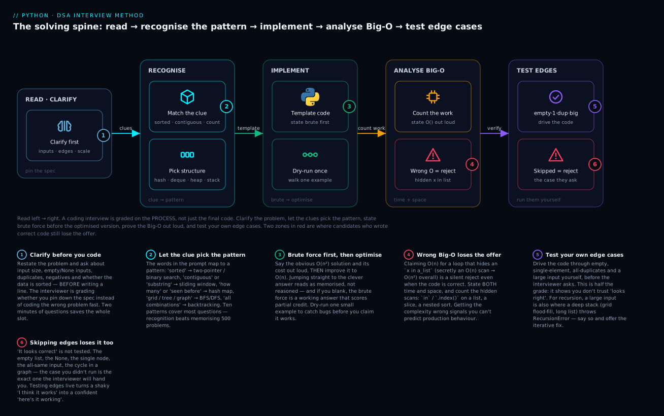
The six badges narrate the whole method: clarify before coding so you solve the right problem (1); let the clue in the prompt pick the pattern (2); state brute force before the optimised version so your reasoning is visible (3); a wrong Big-O is a silent reject even when the code runs (4); test empty, single, duplicate and large inputs yourself (5); and the edge case you skip is precisely the one the interviewer will hand you (6). Run the spine in order every time and you convert “I hope I get a problem I’ve seen” into “I have a process for problems I haven’t.”
The whole point of a method is that you run it when you’re scared. Practise it on easy problems until it’s automatic, so that on the hard one — when your heart rate is up and the editor is blank — your hands know the first move: restate the problem and ask a question.
Complexity first: state time and space out loud
Before the patterns, internalise the one sentence you must be able to say about every solution: “this is O() time and O() space.” Interviewers ask it about every answer, and getting it wrong is worse than not optimising, because it signals you can’t predict how your code behaves in production. This is a fast recap; the full treatment is in the complexity lesson.
Big-O is a growth rate, not a running time: it says what happens to the work when the input gets 10× bigger, ignoring constants and lower-order terms because those never change the shape of the curve. Here is the ladder, with the vocabulary you’ll use to describe interview solutions:
| Class | Name | You get it from | n=1,000,000 feels |
|---|---|---|---|
| O(1) | Constant | Hash lookup, xs[i], .append(), arithmetic |
Instant, at any size |
| O(log n) | Logarithmic | Binary search, bisect, balanced-tree ops |
20 steps for a million |
| O(n) | Linear | One pass — for, sum(), one sweep of the input |
Fast; the usual target |
| O(n log n) | Linearithmic | sorted(), heap-based, divide-and-conquer |
The best you can do for comparison sorting |
| O(n²) | Quadratic | Nested loops, all-pairs, x in list inside a loop |
The wall — minutes at a million |
| O(2ⁿ) / O(n!) | Exponential / factorial | Naive recursion, all subsets, all permutations | Hopeless past n≈20–40 |
Two rules read any snippet’s complexity. Nested loops multiply (a loop over n inside a loop over n is O(n²)); sequential steps add, so the biggest one wins (an O(n) pass then an O(n log n) sort is O(n log n)). The trap that fails interviews is the hidden loop: if x in a_list looks like one operation but is an O(n) scan, so wrapping it in a for is a secret O(n²). We’ll flag it every time it appears.
Space complexity is the same idea for memory — the extra memory the algorithm allocates beyond the input. A set of seen values is O(n) space; two integer pointers are O(1); the call stack of a recursion n deep is O(n) space even if it looks like it allocates nothing. Interviewers grade space too, and the classic answer is a time–space trade-off: “I can do this in O(n) time if I spend O(n) space on a hash set, or O(1) space if I sort first and accept O(n log n) time.” Naming that trade-off out loud is often the exact thing they’re listening for.
Here’s how to state complexity for a real solution, so the phrasing is muscle memory:
| Solution | Time | Space | How you’d say it |
|---|---|---|---|
| Two nested loops over the array | O(n²) | O(1) | “Quadratic time, constant extra space” |
| One pass building a hash set | O(n) | O(n) | “Linear time, linear space — I trade memory for speed” |
| Sort, then one linear pass | O(n log n) | O(1)–O(n) | “n-log-n dominated by the sort, then linear” |
| Two pointers on a sorted array | O(n) | O(1) | “Linear time, constant space — no extra structure” |
| Binary search | O(log n) | O(1) | “Logarithmic — I halve the search space each step” |
| BFS/DFS over a graph | O(V + E) | O(V) | “Linear in vertices plus edges; the visited set is O(V)” |
| Recursion computing all subsets | O(2ⁿ) | O(n) stack | “Exponential — there are 2ⁿ subsets; stack depth is n” |
You cannot state a solution’s complexity without knowing what the operations inside it cost — and in Python the surprises live in the built-ins. This is the table to burn into memory, because half of all mis-stated complexities come from treating an O(n) operation as O(1). Times are the honest asymptotic cost (some measured on CPython 3.12 at n=1,000,000 in the complexity lesson):
| Operation | Complexity | The interview trap |
|---|---|---|
xs[i], len(xs), xs.append(v), xs.pop() |
O(1) | These are free — build a list by appending, always |
x in a_list, a_list.index(x), .count(), .remove() |
O(n) | The #1 hidden scan — quadratic when inside a loop |
a_list.insert(0, v), a_list.pop(0) |
O(n) | Every element shifts — never use a list as a queue |
xs.sort() / sorted(xs) |
O(n log n) | A “clever” one-liner that sorts is not O(n) |
x in a_set, x in a_dict, d[k], s.add(x) |
O(1) avg | 326,000× faster than list membership at n=1M |
deque.appendleft(x), deque.popleft() |
O(1) | Why BFS uses deque, not list.pop(0) |
heapq.heappush / heappop |
O(log n) | Top-k in O(n log k); the heap peek heap[0] is O(1) |
bisect.bisect_left(a, x) |
O(log n) | Binary search on a sorted list, in C |
"".join(parts) |
O(n) | The right way to build a string from pieces |
Slicing xs[a:b] |
O(k) | Copies k elements — a hidden cost in a loop |
The three rows that decide interviews are the O(n) list operations pretending to be cheap: in, .index(), and pop(0). Every one is a loop Python runs on your behalf, and every one turns a linear-looking solution quadratic when it sits inside a for. If you take one reference table from this lesson, take this one.
The ten patterns
Each pattern below follows the same shape: the clue that triggers it, a reusable template, a solved example that was actually run, and its complexity. Learn to recognise the clue and the code becomes mechanical. First, the recognition table — the single most valuable thing to internalise, because in the interview you read the prompt, spot the clue, and the pattern names itself.
| Clue in the prompt | Pattern | Typical complexity |
|---|---|---|
| “Pair / two numbers that sum to…”, “seen before?”, “count of each” | Hash map | O(n) time, O(n) space |
| Array is sorted; “pair”, “reverse in place”, “remove duplicates”, “palindrome” | Two pointers | O(n) time, O(1) space |
| Contiguous subarray / substring; “longest / max / min window”, “of size k” | Sliding window | O(n) time |
| “Sum of a range”, “subarray summing to k”, repeated range queries | Prefix sum | O(n) build, O(1) query |
| Data is sorted; “find target”; or “minimum X that works” (answer space) | Binary search | O(log n) time |
| “Matching / balanced brackets”, “next greater / warmer”, “nearest smaller” | Stack (often monotonic) | O(n) time |
| Linked list; “cycle?”, “middle”, “nth from end”, “reverse” | Fast/slow pointers | O(n) time, O(1) space |
| Tree; “level order”, “depth”, “validate BST”, “path” | Tree DFS / BFS | O(n) time |
| Graph or grid; “connected”, “shortest path (unweighted)”, “islands”, “reachable” | BFS / DFS + visited | O(V+E) time |
| “All subsets / permutations / combinations”, “generate every…” | Backtracking | O(2ⁿ) or O(n!) |
| “Fewest / most / number of ways”, overlapping subproblems, “min coins”, “climb stairs” | Dynamic programming | O(n·states) |
To make the “many problems, one pattern” thesis concrete, here are famous questions grouped by the pattern that solves them. Notice how different the prompts look and how few the patterns are — this is the whole reason recognition beats memorisation:
| Pattern | Canonical problems it solves (different prompts, same tool) |
|---|---|
| Hash map | Two Sum · Group Anagrams · Valid Anagram · Contains Duplicate · Top K Frequent · First Unique Character |
| Two pointers | Two Sum II (sorted) · Valid Palindrome · Container With Most Water · 3Sum · Remove Duplicates · Move Zeroes |
| Sliding window | Longest Substring Without Repeats · Max Subarray of Size K · Minimum Window Substring · Longest Repeating Char Replacement |
| Prefix sum | Subarray Sum Equals K · Range Sum Query · Product of Array Except Self · Contiguous Array |
| Binary search | Search in Rotated Sorted Array · Find Minimum · Koko Eating Bananas · Median of Two Sorted Arrays · Sqrt(x) |
| Stack | Valid Parentheses · Daily Temperatures · Next Greater Element · Min Stack · Largest Rectangle in Histogram |
| Fast/slow pointers | Linked List Cycle · Middle of the List · Remove Nth From End · Reorder List · Happy Number |
| Tree DFS/BFS | Max Depth · Validate BST · Level Order · Path Sum · Lowest Common Ancestor · Serialize/Deserialize |
| Graph BFS/DFS | Number of Islands · Clone Graph · Course Schedule · Rotting Oranges · Word Ladder · Pacific Atlantic |
| Backtracking | Subsets · Permutations · Combination Sum · Word Search · N-Queens · Generate Parentheses |
| Dynamic programming | Climbing Stairs · Coin Change · House Robber · Longest Increasing Subsequence · Edit Distance · Word Break |
Roughly sixty of the most-asked interview problems, and every one of them is a member of this eleven-row family. Learn the family, and each new problem is a matching exercise.
1. Hash map / frequency counting
Clue: you need to know “have I seen this value?”, “what’s its partner?”, or “how many of each?” — and you’re tempted to write a nested loop to find out. A hash map (dict or set) turns that O(n²) search into O(n) by trading memory for constant-time lookups. This is the most common pattern in interviews, full stop.
Template — the two-sum, the single most-asked question. The insight: instead of asking “is my partner somewhere ahead of me?” (which forces an inner loop), ask “did my partner already go past?” — which a dict answers in O(1).
def two_sum(nums, target):
    seen = {}                          # value -> index we saw it at
    for i, n in enumerate(nums):
        want = target - n
        if want in seen:               # O(1): did the partner already appear?
            return [seen[want], i]
        seen[n] = i
    return None
Run it against normal and edge cases:
print(two_sum([2, 7, 11, 15], 9))     # => [0, 1]
print(two_sum([3, 2, 4], 6))          # => [1, 2]
print(two_sum([3, 3], 6))             # => [0, 1]   (duplicate values, still works)
print(two_sum([1, 2, 3], 100))        # => None     (no pair)
print(two_sum([], 0))                 # => None     (empty input)
Complexity: O(n) time — one pass — and O(n) space for the dict. The brute-force nested-loop version is O(n²) time but O(1) space; naming that trade-off (“I’ll spend O(n) memory to drop from quadratic to linear time”) is the point. Measured, hash vs brute, worst case (no pair exists so both scan fully):
| n | Hash O(n) | Growth | Brute O(n²) | Growth | Speedup |
|---|---|---|---|---|---|
| 1,000 | 50.4 µs | — | 15.32 ms | — | 304× |
| 2,000 | 102.0 µs | ×2.02 | 62.24 ms | ×4.06 | 610× |
| 4,000 | 206.4 µs | ×2.02 | 249.75 ms | ×4.01 | 1,210× |
| 8,000 | 415.7 µs | ×2.01 | 1002.67 ms | ×4.01 | 2,412× |
The growth columns are the Big-O, measured: hash doubles (×2, linear), brute quadruples (×4, quadratic), and the gap widens forever. Two more problems, same pattern:
from collections import Counter, defaultdict

def is_anagram(s, t):
    return Counter(s) == Counter(t)    # equal letter frequencies

print(is_anagram("listen", "silent"))  # => True
print(is_anagram("rat", "car"))        # => False

def group_anagrams(words):
    groups = defaultdict(list)
    for w in words:
        key = "".join(sorted(w))       # canonical form: sorted letters
        groups[key].append(w)
    return list(groups.values())

print(group_anagrams(["eat", "tea", "tan", "ate", "nat", "bat"]))
# => [['eat', 'tea', 'ate'], ['tan', 'nat'], ['bat']]
Counter and defaultdict are your interview workhorses — more on them in the toolkit section. The dict/set behaviour underneath (hashing, why keys must be immutable) is covered in Dictionaries & Sets: Key/Value & Membership.
2. Two pointers
Clue: the array is sorted (or you’re working from both ends), and you’re comparing or converging — “find a pair,” “reverse in place,” “remove duplicates,” “is it a palindrome.” Two indices walking the array replace a nested loop: each step rules out a candidate, giving O(n) time and O(1) space (no extra structure). When the data is sorted, two pointers often beats even the hash map on space.
Template — pair with a target sum (the sorted twin of two-sum). Walk from both ends; the sortedness tells you which pointer to move:
def two_sum_sorted(nums, target):
    lo, hi = 0, len(nums) - 1
    while lo < hi:
        s = nums[lo] + nums[hi]
        if s == target:
            return [lo, hi]
        if s < target:
            lo += 1          # need a bigger sum -> raise the low end
        else:
            hi -= 1          # need a smaller sum -> lower the high end
    return None

print(two_sum_sorted([2, 7, 11, 15], 9))       # => [0, 1]
print(two_sum_sorted([1, 3, 4, 5, 7, 11], 9))  # => [2, 3]   (4 + 5)
print(two_sum_sorted([1, 2, 3], 100))          # => None
Palindrome check — pointers from both ends, meeting in the middle:
def is_palindrome(s):
    cleaned = [c.lower() for c in s if c.isalnum()]   # ignore case & punctuation
    lo, hi = 0, len(cleaned) - 1
    while lo < hi:
        if cleaned[lo] != cleaned[hi]:
            return False
        lo += 1
        hi -= 1
    return True

print(is_palindrome("A man, a plan, a canal: Panama"))  # => True
print(is_palindrome("race a car"))                      # => False
print(is_palindrome(""))                                # => True   (empty is a palindrome)
print(is_palindrome("a"))                               # => True
In-place dedupe of a sorted array — a slow pointer marks where to write, a fast pointer scans ahead. This is the “fast/slow on an array” flavour:
def remove_duplicates(nums):
    """Compact uniques to the front of a SORTED list; return the count."""
    if not nums:
        return 0
    write = 1                          # slow: next slot to fill
    for read in range(1, len(nums)):   # fast: scans every element
        if nums[read] != nums[write - 1]:
            nums[write] = nums[read]
            write += 1
    return write

a = [1, 1, 2, 2, 2, 3, 4, 4]
k = remove_duplicates(a)
print(k, a[:k])                        # => 4 [1, 2, 3, 4]
Complexity: all three are O(n) time, O(1) extra space. That constant space is the selling point over a hash map when the input is already sorted.
| Two-pointer flavour | Pointers start | Move rule | Example |
|---|---|---|---|
| Converging (opposite ends) | lo=0, hi=n-1 |
Move the end that improves the condition | Pair sum, palindrome, container-with-most-water |
| Fast/slow (same end) | slow=0, fast=1 |
fast scans; slow marks a write/boundary |
In-place dedupe, move zeroes, partition |
| Two sequences | one per list | Advance the smaller | Merge sorted lists, intersection |
3. Sliding window
Clue: a contiguous subarray or substring, and you want the longest / shortest / max / min of something — “max sum of k consecutive,” “longest substring without repeats.” Instead of recomputing each window from scratch (O(n·k)), you slide: add the entering element, remove the leaving one, updating the answer in O(1) per step. Total O(n).
Fixed window (size k is given) — add the new, drop the old:
def max_sum_k(nums, k):
    if len(nums) < k:
        return None
    window = sum(nums[:k])             # first window, computed once
    best = window
    for i in range(k, len(nums)):
        window += nums[i] - nums[i - k]  # +entering, -leaving: O(1) per step
        best = max(best, window)
    return best

print(max_sum_k([2, 1, 5, 1, 3, 2], 3))   # => 9   (5 + 1 + 3)
print(max_sum_k([1, 2], 3))                # => None (window bigger than list)
Variable window (grow/shrink to satisfy a condition) — the harder, more common flavour. Longest substring without repeating characters: expand the right edge each step; when a repeat appears, jump the left edge past the previous occurrence:
def longest_unique_substring(s):
    last_seen = {}                     # char -> its most recent index
    start = 0                          # left edge of the window
    best = 0
    for i, c in enumerate(s):
        if c in last_seen and last_seen[c] >= start:
            start = last_seen[c] + 1   # shrink from the left, past the repeat
        last_seen[c] = i
        best = max(best, i - start + 1)
    return best

for t in ["abcabcbb", "bbbbb", "pwwkew", "", "au", "dvdf", "tmmzuxt"]:
    print(f"{t!r:12} -> {longest_unique_substring(t)}")
'abcabcbb'   -> 3
'bbbbb'      -> 1
'pwwkew'     -> 3
''           -> 0
'au'         -> 2
'dvdf'       -> 3
'tmmzuxt'    -> 5
(Both were cross-checked against a brute-force O(n²) reference on 3,000 random inputs — they agree.) Complexity: O(n) time — each element enters and leaves the window at most once — and O(k) space for the window’s contents (O(1) for the fixed-sum version). Measured against recomputing each window, with k = n/2:
| n | Window O(n) | Recompute O(n·k) | Speedup |
|---|---|---|---|
| 2,000 | 118.8 µs | 3.66 ms | 31× |
| 4,000 | 239.1 µs | 14.41 ms | 60× |
| 8,000 | 493.8 µs | 66.14 ms | 134× |
The speedup grows with n because the naive version is O(n·k) = O(n²) when k scales with n, while the window stays linear.
| Window type | You know | You track | Answer is |
|---|---|---|---|
| Fixed | The window size k | A running sum/count | Best over all windows of size k |
| Variable | A condition to satisfy | Left+right edges, a dict/counter of contents | Longest/shortest window meeting the condition |
4. Prefix sum
Clue: repeated “sum of a range” queries, or “how many subarrays sum to k.” Precompute cumulative sums once; then any range sum is a subtraction. prefix[j] - prefix[i] is the sum of nums[i:j] in O(1), after an O(n) build.
def build_prefix(nums):
    prefix = [0] * (len(nums) + 1)     # prefix[0] = 0 (empty prefix)
    for i, n in enumerate(nums):
        prefix[i + 1] = prefix[i] + n
    return prefix

nums = [3, 1, 4, 1, 5, 9, 2, 6]
prefix = build_prefix(nums)
print(prefix)                          # => [0, 3, 4, 8, 9, 14, 23, 25, 31]
print(prefix[5] - prefix[2])           # => 10   (sum of nums[2:5] = 4+1+5)
The killer application combines prefix sums with a hash map: count subarrays summing to k in one pass. For each running total, ask “how many earlier prefixes were exactly running - k?” — because each such prefix marks the start of a subarray summing to k:
from collections import defaultdict

def subarray_sum_equals_k(nums, k):
    count = running = 0
    seen = defaultdict(int)
    seen[0] = 1                        # one empty prefix, sum 0
    for n in nums:
        running += n
        count += seen[running - k]     # earlier prefixes that complete a k-sum
        seen[running] += 1
    return count

print(subarray_sum_equals_k([1, 1, 1], 2))          # => 2
print(subarray_sum_equals_k([1, 2, 3], 3))          # => 2   ([1,2] and [3])
print(subarray_sum_equals_k([1, -1, 1, -1], 0))     # => 4   (handles negatives)
The intuition for the one-pass version is worth slowing down on, because it’s the trick that recurs across dozens of “count the subarrays” problems. A contiguous subarray’s sum is the difference of two running prefixes: the sum of nums[i:j] equals running_at_j - running_at_i. So a subarray ending at the current position sums to k exactly when some earlier prefix equalled running - k. Rather than search for those earlier prefixes (a loop), you keep a running tally of how many times each prefix value has occurred, and at each step you simply look up running - k — O(1). The seen[0] = 1 seed accounts for subarrays that start at index 0, whose “earlier prefix” is the empty prefix of sum 0. Recognise “count / find contiguous subarrays with sum k” and this template is the answer.
Complexity: O(n) time, O(n) space — one pass, a dict of prefix counts. The brute force is O(n²) (every start/end pair). Note this handles negative numbers, where a sliding window would not work — a window assumes growing the window grows the sum, which negatives break. Recognising “sliding window needs non-negative; this has negatives, so prefix sum + hash” is exactly the adaptation an interviewer wants to see.
5. Binary search
Clue, form one: the data is sorted and you’re searching for a target — O(log n), 20 steps for a million. Clue, form two (the one that separates candidates): you’re asked for the “minimum/maximum value that satisfies some condition,” and that condition is monotonic (once true, it stays true) — you can binary-search the answer space even though there’s no array to search.
Form one — search a sorted array. Three lines hold every bug, so name them: while lo <= hi (a one-element window is still valid), lo = mid + 1 / hi = mid - 1 (you already checked mid, exclude it):
def binary_search(items, target):
    lo, hi = 0, len(items) - 1
    while lo <= hi:                    # <= : a 1-item window can still hold the answer
        mid = (lo + hi) // 2
        if items[mid] == target:
            return mid
        if items[mid] < target:
            lo = mid + 1               # answer is in the right half
        else:
            hi = mid - 1               # answer is in the left half
    return -1                          # window emptied -> absent

evens = list(range(0, 100, 2))
print(binary_search(evens, 42))        # => 21
print(binary_search(evens, 43))        # => -1   (odd, not present)
print(binary_search([], 5))            # => -1   (empty)
print(binary_search([5], 5))           # => 0    (single element)
Form two — binary search on the answer. “Koko eats bananas”: given piles and h hours, find the minimum eating speed that finishes in time. The answer is a speed somewhere in [1, max(piles)]; “can she finish at speed s?” is monotonic (faster is never worse), so binary-search the speed:
import math

def min_eating_speed(piles, h):
    def hours_at(speed):
        return sum(math.ceil(p / speed) for p in piles)
    lo, hi = 1, max(piles)             # the answer space, not an array
    while lo < hi:
        mid = (lo + hi) // 2
        if hours_at(mid) <= h:         # fast enough -> try slower (search left)
            hi = mid
        else:
            lo = mid + 1               # too slow -> must speed up
    return lo                          # lo == hi: the smallest feasible speed

print(min_eating_speed([3, 6, 7, 11], 8))       # => 4
print(min_eating_speed([30, 11, 23, 4, 20], 5)) # => 30
print(min_eating_speed([30, 11, 23, 4, 20], 6)) # => 23
The mental leap in form two is realising there’s a sorted structure you never built: the sequence of yes/no answers to “can she finish at speed s?” runs no, no, …, no, yes, yes, …, yes as s increases, because a faster speed is never worse. That monotone boundary is exactly what binary search finds — and the array you’re searching is the imaginary list of feasibility answers, not the piles. Whenever a problem asks for the smallest or largest value that makes some test pass, and the test is monotonic, you can binary-search the value even though there’s nothing sorted in the input. The tell is the phrasing “minimum X such that…” or “maximum X such that…”; write the feasible(mid) check first, confirm it’s monotonic, then wrap the standard lo/hi loop around it. This single insight turns a class of problems that look like they need clever maths into the binary search you already know.
(Both were checked against linear-scan brute forces — exhaustively for form one, on 500 random cases for form two.) Complexity: form one is O(log n); form two is O(n log(max)) — log(max(piles)) binary-search steps, each doing an O(n) feasibility check. The precondition for form one is sorted data — on unsorted input binary search doesn’t raise, it silently returns wrong answers, which is why it’s a favourite interviewer trap.
| Binary search on an array | Binary search on the answer | |
|---|---|---|
| What you search | Indices [0, n-1] |
A value range [lo, hi] |
| Precondition | Array is sorted | The “does X work?” test is monotonic |
| The comparison | items[mid] vs target |
feasible(mid) — a function you write |
| Loop invariant | Target in [lo, hi] if present |
Answer in [lo, hi] |
| Cost per step | O(1) | O(n) (the feasibility check) |
| Clue words | “sorted”, “find target” | “minimum/maximum X such that…” |
6. Stack
Clue: matching or nesting (“balanced brackets”), or “next greater / warmer / smaller element.” A stack (just a Python list with append/pop) tracks “the most recent unresolved thing” — LIFO order.
Valid parentheses — push openers, pop-and-match on closers:
def is_valid_parens(s):
    pairs = {")": "(", "]": "[", "}": "{"}
    stack = []
    for c in s:
        if c in "([{":
            stack.append(c)
        elif c in ")]}":
            if not stack or stack.pop() != pairs[c]:  # nothing to match, or wrong match
                return False
    return not stack                   # leftover openers -> unbalanced

for t in ["()", "()[]{}", "(]", "([)]", "{[]}", "", "(", ")"]:
    print(f"{t!r:8} -> {is_valid_parens(t)}")
'()'     -> True
'()[]{}' -> True
'(]'     -> False
'([)]'   -> False
'{[]}'   -> True
''       -> True
'('      -> False
')'      -> False
Monotonic stack — a stack kept sorted (here, decreasing) so you can answer “next greater element” in O(n). Daily temperatures: for each day, how many days until a warmer one? Keep a stack of indices whose temperature is still waiting for something warmer:
def daily_temperatures(temps):
    answer = [0] * len(temps)
    stack = []                         # indices with temps still decreasing
    for i, t in enumerate(temps):
        while stack and temps[stack[-1]] < t:   # t resolves everything cooler
            j = stack.pop()
            answer[j] = i - j          # days waited
        stack.append(i)
    return answer

print(daily_temperatures([73, 74, 75, 71, 69, 72, 76, 73]))
# => [1, 1, 4, 2, 1, 1, 0, 0]
Complexity: valid-parens is O(n) time, O(n) space (worst case all openers). The monotonic stack looks like O(n²) because of the inner while, but it’s O(n): each index is pushed once and popped at most once, so the total work across all iterations is linear. That amortised argument — “each element is pushed and popped once” — is exactly what an interviewer wants to hear when they ask about the nested loop’s cost.
7. Linked list: fast and slow pointers
Clue: a linked list and a question about position or structure — “find the middle,” “is there a cycle,” “nth from the end,” “reverse it.” Two pointers moving at different speeds (Floyd’s tortoise and hare) answer these in one pass, O(1) space. First, a minimal node and helpers:
class ListNode:
    def __init__(self, val=0, nxt=None):
        self.val = val
        self.next = nxt

def build_list(values):
    head = None
    for v in reversed(values):
        head = ListNode(v, head)
    return head
Middle of the list — slow moves 1, fast moves 2; when fast hits the end, slow is at the middle:
def middle_node(head):
    slow = fast = head
    while fast and fast.next:
        slow = slow.next               # 1 step
        fast = fast.next.next          # 2 steps
    return slow

print(middle_node(build_list([1, 2, 3, 4, 5])).val)     # => 3
print(middle_node(build_list([1, 2, 3, 4, 5, 6])).val)  # => 4  (second middle)
print(middle_node(build_list([1])).val)                 # => 1
Cycle detection — if fast ever catches slow, there’s a loop; if fast reaches the end, there isn’t:
def has_cycle(head):
    slow = fast = head
    while fast and fast.next:
        slow = slow.next
        fast = fast.next.next
        if slow is fast:               # the hare lapped the tortoise
            return True
    return False

lst = build_list([1, 2, 3, 4])
print(has_cycle(lst))                  # => False

# splice the tail back to the 2nd node to make a cycle
tail = lst
while tail.next:
    tail = tail.next
tail.next = lst.next
print(has_cycle(lst))                  # => True
print(has_cycle(None))                 # => False  (empty list)
Reverse a linked list — the other must-know; three pointers flipping next one link at a time:
def reverse_list(head):
    prev = None
    while head:
        nxt = head.next                # remember the rest
        head.next = prev               # flip this link backwards
        prev = head                    # advance prev
        head = nxt                     # advance head
    return prev                        # new head is the old tail

def to_pylist(head):
    out = []
    while head:
        out.append(head.val); head = head.next
    return out

print(to_pylist(reverse_list(build_list([1, 2, 3, 4, 5]))))  # => [5, 4, 3, 2, 1]
print(to_pylist(reverse_list(build_list([]))))               # => []
Complexity: all O(n) time, O(1) space — the whole point of the pointer trick is that it needs no extra list. The while fast and fast.next guard is the edge-case workhorse: it handles empty lists and odd/even lengths without a special case. Test empty and single-node inputs every time — they’re where linked-list solutions crash with AttributeError: 'NoneType' object has no attribute 'next'.
8. Trees: DFS and BFS
Clue: a binary tree and a question about traversal order, depth, or a property like “is this a valid BST.” Two engines cover almost everything: DFS (depth-first — recursion or an explicit stack) and BFS (breadth-first / level-order — a queue).
class TreeNode:
    def __init__(self, val=0, left=None, right=None):
        self.val, self.left, self.right = val, left, right

#         4
#        / \        Build a small BST to test against.
#       2   6
#      / \ / \
#     1  3 5  7
root = TreeNode(4,
                TreeNode(2, TreeNode(1), TreeNode(3)),
                TreeNode(6, TreeNode(5), TreeNode(7)))
DFS, recursive — the natural expression; in-order on a BST yields sorted values:
def inorder_recursive(node, out=None):
    if out is None:
        out = []
    if node:
        inorder_recursive(node.left, out)
        out.append(node.val)           # visit between the subtrees = in-order
        inorder_recursive(node.right, out)
    return out

print(inorder_recursive(root))         # => [1, 2, 3, 4, 5, 6, 7]
DFS, iterative — the same traversal with an explicit stack. Worth knowing because deep trees blow the recursion stack (Python’s limit is 1000), and interviewers love asking for the iterative version:
def inorder_iterative(node):
    out, stack = [], []
    while node or stack:
        while node:                    # dive left, stacking as you go
            stack.append(node)
            node = node.left
        node = stack.pop()             # backtrack to the last unvisited
        out.append(node.val)
        node = node.right              # then explore right
    return out

print(inorder_iterative(root))         # => [1, 2, 3, 4, 5, 6, 7]
print(inorder_recursive(root) == inorder_iterative(root))  # => True
BFS, level-order — a queue (deque), processing one full level per outer iteration. The for _ in range(len(q)) snapshot is the trick that groups nodes by level:
from collections import deque

def level_order(root):
    if not root:
        return []
    result, q = [], deque([root])
    while q:
        level = []
        for _ in range(len(q)):        # exactly this level's nodes
            node = q.popleft()
            level.append(node.val)
            if node.left:  q.append(node.left)
            if node.right: q.append(node.right)
        result.append(level)
    return result

print(level_order(root))               # => [[4], [2, 6], [1, 3, 5, 7]]
print(level_order(None))               # => []
Validate a BST — the classic trap: it’s not enough to check each node against its children; every node must fall within a range narrowed by its ancestors:
def is_valid_bst(node, lo=float("-inf"), hi=float("inf")):
    if not node:
        return True
    if not (lo < node.val < hi):
        return False
    return (is_valid_bst(node.left, lo, node.val) and    # right bound tightens
            is_valid_bst(node.right, node.val, hi))       # left bound tightens

print(is_valid_bst(root))              # => True
bad = TreeNode(4, TreeNode(2, TreeNode(1), TreeNode(5)), TreeNode(6))  # 5 sits left of 4
print(is_valid_bst(bad))               # => False
Complexity: every traversal is O(n) time (each node once). Space is O(h) for DFS (recursion/stack depth = tree height, O(log n) balanced, O(n) degenerate) and O(w) for BFS (queue holds the widest level, up to O(n)).
| Traversal | Engine | Order | Use for |
|---|---|---|---|
| In-order (L, node, R) | DFS | Sorted, for a BST | Validate/serialize a BST |
| Pre-order (node, L, R) | DFS | Root first | Copy a tree, serialize |
| Post-order (L, R, node) | DFS | Children first | Delete a tree, compute sizes/heights |
| Level-order | BFS | Top to bottom, left to right | Shortest depth, level grouping |
9. Graphs: BFS/DFS, visited sets, grids
Clue: a graph or a grid (which is a graph in disguise — each cell connects to its neighbours), and a question about reachability, connectivity, shortest unweighted path, or “islands.” Same two engines as trees, plus one non-negotiable addition: a visited set, because graphs have cycles and without it you loop forever.
from collections import deque

graph = {
    "A": ["B", "C"], "B": ["A", "D", "E"], "C": ["A", "F"],
    "D": ["B"], "E": ["B", "F"], "F": ["C", "E"],
}

def bfs(graph, start):
    visited = {start}                  # mark BEFORE enqueuing to avoid duplicates
    q = deque([start])
    order = []
    while q:
        node = q.popleft()
        order.append(node)
        for nb in graph[node]:
            if nb not in visited:      # the visited set = no infinite loop
                visited.add(nb)
                q.append(nb)
    return order

def dfs(graph, start):
    visited, order = set(), []
    def walk(node):
        visited.add(node)
        order.append(node)
        for nb in graph[node]:
            if nb not in visited:
                walk(nb)
    walk(start)
    return order

print(bfs(graph, "A"))                 # => ['A', 'B', 'C', 'D', 'E', 'F']
print(dfs(graph, "A"))                 # => ['A', 'B', 'D', 'E', 'F', 'C']
BFS versus DFS is a real choice, not a coin flip: BFS explores in rings of increasing distance, so it finds the shortest path in an unweighted graph; DFS plunges down one branch first, so it’s the natural fit for “does a path exist,” cycle detection, and topological ordering. The clue “shortest / fewest steps” means BFS; “any path / all paths / connectivity” leans DFS. Know how the graph is handed to you, too, because it changes the neighbour lookup:
| Representation | Shape | Neighbour lookup | When you’ll see it |
|---|---|---|---|
| Adjacency list | {node: [neighbours]} (a defaultdict(list)) |
O(degree) | The default — sparse graphs, most interview inputs |
| Adjacency matrix | grid[i][j] = 1 if edge |
O(1) check, O(V) to list | Dense graphs; “is there an edge?” queries |
| Edge list | [(u, v), …] |
O(E) — usually converted first | Given as input; build an adjacency list from it |
| Implicit / grid | 2-D grid; neighbours are (r±1, c), (r, c±1) |
O(1), computed | Islands, mazes, flood fill — a graph in disguise |
The grid row is the one interviews lean on hardest: the moment you see a 2-D grid and “connected regions” or “shortest path through cells,” translate it to a graph in your head — cells are nodes, adjacent cells are edges — and the same BFS/DFS you already know applies unchanged.
Number of islands — the canonical grid problem. Scan every cell; each unvisited land cell starts a new island, and a flood fill (DFS here) sinks its whole connected component so you don’t count it twice:
def num_islands(grid):
    if not grid:
        return 0
    rows, cols = len(grid), len(grid[0])
    count = 0
    def sink(r, c):
        if r < 0 or r >= rows or c < 0 or c >= cols or grid[r][c] != "1":
            return                     # off-grid or water or already sunk
        grid[r][c] = "0"               # mark visited by sinking the land
        sink(r + 1, c); sink(r - 1, c); sink(r, c + 1); sink(r, c - 1)
    for r in range(rows):
        for c in range(cols):
            if grid[r][c] == "1":
                count += 1
                sink(r, c)
    return count

g1 = [list("11110"), list("11010"), list("11000"), list("00000")]
print(num_islands(g1))                 # => 1
g2 = [list("11000"), list("11000"), list("00100"), list("00011")]
print(num_islands(g2))                 # => 3
print(num_islands([]))                 # => 0
print(num_islands([list("1")]))        # => 1
Complexity: BFS/DFS are O(V + E) — every vertex and edge visited once; the grid version is O(rows × cols). Space is O(V) for the visited set (or, in the grid, O(1) extra if you’re allowed to mutate the grid, plus the recursion/queue).
⚠️ The recursive flood fill has a hidden failure: on a large solid island the recursion can go tens of thousands deep and blow the stack. Measured — a 200×200 all-land grid raises RecursionError with the recursive version, while a BFS version using a deque returns 1 cleanly. For big grids, use the iterative BFS/DFS. Mentioning this trade-off unprompted is a strong signal in an interview.
10. Backtracking (and a note on dynamic programming)
Clue: “generate all subsets / permutations / combinations,” “find every valid arrangement.” Backtracking builds candidates incrementally with choose → explore → un-choose: make a move, recurse, then undo the move to try the next. The un-choose is what makes it back-tracking.
def subsets(nums):
    result, path = [], []
    def backtrack(start):
        result.append(path[:])         # snapshot: COPY the path, not a reference
        for i in range(start, len(nums)):
            path.append(nums[i])       # choose
            backtrack(i + 1)           # explore with this choice
            path.pop()                 # un-choose (backtrack)
    backtrack(0)
    return result

print(subsets([1, 2, 3]))
# => [[], [1], [1, 2], [1, 2, 3], [1, 3], [2], [2, 3], [3]]
print(len(subsets([1, 2, 3])))         # => 8   (= 2^3)

def permutations(nums):
    result, path = [], []
    used = [False] * len(nums)
    def backtrack():
        if len(path) == len(nums):
            result.append(path[:])
            return
        for i in range(len(nums)):
            if used[i]:
                continue
            used[i] = True; path.append(nums[i])
            backtrack()
            path.pop(); used[i] = False   # un-choose both
    backtrack()
    return result

print(permutations([1, 2, 3]))
# => [[1, 2, 3], [1, 3, 2], [2, 1, 3], [2, 3, 1], [3, 1, 2], [3, 2, 1]]
print(len(permutations([1, 2, 3])))    # => 6   (= 3!)
⚠️ The path[:] copy is the bug that catches everyone: append path directly and every entry in result is the same list object, which ends up empty after all the pops. I ran the buggy version — result.append(path) — and it returns [[], [], [], [], [], [], [], []] instead of the real subsets. Always snapshot the mutable state you’re collecting.
Complexity: subsets is O(2ⁿ) (there are 2ⁿ of them), permutations O(n!) — inherently exponential, because the output is exponential. That’s fine when n is small (the constraint that makes these tractable); if n is large, the problem isn’t really “generate all,” and you’ve misread it.
Dynamic programming is the pattern for “fewest / most / number of ways” with overlapping subproblems — the same sub-answer is needed many times. The move is to remember it. Naive recursive Fibonacci-style “climbing stairs” recomputes the same values exponentially; memoisation caches them, and functools.lru_cache makes that a one-line decorator:
from functools import lru_cache

def climb_naive(n):                    # O(2^n): recomputes everything
    if n <= 2:
        return n
    return climb_naive(n - 1) + climb_naive(n - 2)

@lru_cache(maxsize=None)               # top-down DP: memoise by caching results
def climb_memo(n):                     # O(n): each n computed once
    if n <= 2:
        return n
    return climb_memo(n - 1) + climb_memo(n - 2)

def climb_tab(n):                      # bottom-up DP: O(n) time, O(1) space
    if n <= 2:
        return n
    a, b = 1, 2
    for _ in range(3, n + 1):
        a, b = b, a + b
    return b

print(climb_naive(10), climb_memo(10), climb_tab(10))  # => 89 89 89
print(climb_tab(50))                                   # => 20365011074
The three agree on n = 1…20 (checked). What differs is speed — the same computation, memoised versus recomputed:
| n | Naive O(2ⁿ) | Memoised O(n) | Speedup |
|---|---|---|---|
| 20 | 0.365 ms | 0.03 µs | 11,096× |
| 25 | 4.051 ms | 0.03 µs | 123,845× |
| 30 | 44.991 ms | 0.03 µs | 1,355,426× |
| 32 | 117.519 ms | 0.03 µs | 3,579,156× |
The naive column quadruples-and-then-some per step (that’s 2ⁿ); memoised is flat. The progression naive recursion → add @lru_cache (top-down) → rewrite as a bottom-up table (climb_tab) is the exact story to tell in an interview: recognise overlapping subproblems, memoise to kill the exponential, then optionally tabulate to drop the recursion and the space. Coin change is the other canonical DP — fewest coins to make an amount:
def coin_change(coins, amount):
    INF = float("inf")
    dp = [0] + [INF] * amount          # dp[x] = fewest coins to make x
    for x in range(1, amount + 1):
        for c in coins:
            if c <= x:
                dp[x] = min(dp[x], dp[x - c] + 1)
    return dp[amount] if dp[amount] != INF else -1

print(coin_change([1, 2, 5], 11))      # => 3   (5 + 5 + 1)
print(coin_change([2], 3))             # => -1  (can't make 3 from 2s)
print(coin_change([1], 0))             # => 0
The two ways to write DP are worth contrasting side by side, because interviewers ask you to convert between them:
| Memoisation (top-down) | Tabulation (bottom-up) | |
|---|---|---|
| Shape | Recursion + a cache | A loop filling a dp array |
| Python | @lru_cache on the recursive function |
dp = [...]; iterate from base cases up |
| Derives from | The brute-force recursion, almost unchanged | A recurrence you write deliberately |
| Order | Computes subproblems lazily, as needed | Computes every subproblem, in dependency order |
| Risk | Recursion-depth limit on large inputs | Must get the fill order right |
| Space | Cache + call stack | The table — often shrinkable to O(1) |
| Write it when | You have a working recursion and want it fast | You need to avoid recursion or shrink space |
The interview move is to derive the recursion, slap @lru_cache on it to prove you’ve killed the exponential, then — if asked about space or depth — rewrite as a table and note you only need the last one or two rows (climbing stairs collapses to two variables, O(1) space).
DP has the steepest learning curve of the ten patterns and appears less often in early-career screens — recognise it (the “number of ways / min / max with overlapping subproblems” clue), know memoisation vs tabulation, and have climbing-stairs and coin-change in your fingers. That’s enough for most interviews below the senior algorithm-heavy bar.
Python’s interview toolkit
Python is a superb interview language because its standard library hands you the data structures other candidates hand-roll in C++ or Java. Knowing these cold is a real edge — you write less code, introduce fewer bugs, and finish faster. The catch is a few sharp corners, especially why you must never use list.pop(0) for a queue.
| Tool | Import | What it gives you | Interview use |
|---|---|---|---|
Counter |
from collections import Counter |
Frequency dict; .most_common(k); equality compares counts |
Anagrams, “most frequent”, counting |
defaultdict |
from collections import defaultdict |
Auto-initialising dict — no key-existence checks | Adjacency lists, grouping, counting |
deque |
from collections import deque |
O(1) append/pop at both ends |
BFS queue, sliding window, “last k” |
heapq |
import heapq |
Binary min-heap on a list | Top-k, “k smallest/largest”, Dijkstra, merge-k |
bisect |
import bisect |
Binary search / insertion point in C | Search sorted, “insert keeping sorted”, bucketing |
itertools |
import itertools |
product, permutations, combinations, accumulate |
Generating candidates, prefix sums |
functools.lru_cache |
from functools import lru_cache |
One-line memoisation | Top-down DP |
math |
import math |
inf, ceil, gcd, isqrt |
Sentinels, ceiling division |
Counter and defaultdict eliminate the two most common dict chores:
from collections import Counter, defaultdict

c = Counter("mississippi")
print(c.most_common(2))        # => [('i', 4), ('s', 4)]
print(c["z"])                  # => 0        (missing key -> 0, no KeyError)

graph = defaultdict(list)
graph["A"].append("B")         # no 'if "A" not in graph' dance
print(dict(graph))             # => {'A': ['B']}
deque is non-negotiable for BFS. A Python list is a contiguous array, so list.pop(0) shifts every remaining element left — O(n) — turning an O(V+E) BFS into O(V²). deque.popleft() is O(1). Measured, draining a queue of n items:
from collections import deque
q = deque([1, 2, 3]); q.appendleft(0); q.append(4)
print(list(q))                 # => [0, 1, 2, 3, 4]
print(q.popleft(), q.pop())    # => 0 4   (both O(1))
| n | deque.popleft() |
list.pop(0) |
List slower by |
|---|---|---|---|
| 1,000 | 30.0 µs | 86.0 µs | 3× |
| 2,000 | 61.9 µs | 270.8 µs | 4× |
| 4,000 | 126.3 µs | 942.9 µs | 7× |
| 8,000 | 254.3 µs | 3453.3 µs | 14× |
The “slower by” column grows (3→4→7→14×) — the quadratic fingerprint. At interview scale this is the difference between a passing BFS and one that times out on the large test case. When you write BFS, reach for deque reflexively.
heapq is a min-heap living on a plain list — the tool for “k largest,” “k smallest,” “merge k sorted,” and Dijkstra:
import heapq
nums = [5, 1, 8, 3, 9, 2, 7]
print(heapq.nsmallest(3, nums))   # => [1, 2, 3]
print(heapq.nlargest(3, nums))    # => [9, 8, 7]

def top_k(stream, k):             # size-k min-heap: O(n log k), O(k) space
    heap = []
    for x in stream:
        heapq.heappush(heap, x)
        if len(heap) > k:
            heapq.heappop(heap)   # evict the smallest -> keep the k largest
    return sorted(heap, reverse=True)

print(top_k([5, 1, 8, 3, 9, 2, 7], 3))   # => [9, 8, 7]
It’s a min-heap only; for a max-heap, negate the values on the way in and out. The functions you actually reach for:
| Function | Does | Cost |
|---|---|---|
heapq.heapify(xs) |
Turn a list into a heap in place | O(n) |
heapq.heappush(h, x) |
Add an item, keep heap order | O(log n) |
heapq.heappop(h) |
Remove and return the smallest | O(log n) |
h[0] |
Peek the smallest without removing | O(1) |
heapq.nsmallest(k, xs) / nlargest(k, xs) |
The k smallest / largest | O(n log k) |
heapq.heappushpop(h, x) |
Push then pop in one step | O(log n) |
bisect.bisect_left(a, x) |
First index where x could go (sorted) |
O(log n) |
bisect.bisect_right(a, x) |
Last index where x could go |
O(log n) |
bisect.insort(a, x) |
Insert keeping sorted (search O(log n), shift O(n)) | O(n) |
The size-k min-heap in top_k is the pattern behind “k largest in a stream” and Dijkstra’s frontier — a heap that never grows past k gives O(n log k), beating a full sort’s O(n log n) when k is small. bisect does binary search in C — bisect_left/bisect_right return insertion points; a neat trick is bucketing values (e.g. scores → letter grades) via bisect_right on breakpoints.
The honest meta: it’s a learnable skill
Step back from the code for the uncomfortable truths, because how you practise matters more than how many problems you touch.
Patterns beat problem count. Grinding 500 problems by rote builds a fragile lookup table that shatters when the problem is 10% novel. Studying ~10 patterns until you can recognise them builds a generative skill: you meet an unseen problem, match it to a pattern, adapt the template. The right practice unit is not “do problem #217,” it’s “do three problems that are all sliding-window until the pattern is reflexive, then move on.” Fifteen to twenty well-understood problems per pattern beats hundreds skimmed.
Spaced repetition and re-solving. You have not learned a problem by solving it once. Solve it, then re-solve it three days later from scratch — if you can’t, you memorised, you didn’t learn. Space your review; a problem you can rebuild cold a week later is one you actually own. This is the single biggest efficiency lever in interview prep and the one most people skip.
Mock interviews are not optional. Solving alone in a quiet room trains a different skill from performing under observation with a clock and a stranger. The nerves, the thinking-out-loud, the recovering-from-a-dead-end-gracefully — those only improve under realistic pressure. Do mock interviews (with a friend, a peer, or a platform) until the format stops being the hard part and the problem is. Many strong engineers fail interviews purely on unfamiliarity with the format, which is fixable in a handful of mocks.
It is a learnable skill, not a talent test. This is the most important sentence in the lesson. Nobody is born knowing the sliding-window template. The engineers who pass didn’t have a gift; they practised the patterns and the process deliberately. Impostor feelings are near-universal here and they are not evidence of anything. The interview rewards preparation of a specific kind — and now you know exactly what kind.
When you get stuck — and you will — recover out loud. Freezing silently is the failure; getting stuck is normal and recoverable. Have a mechanical escape sequence: (1) re-read the problem and your examples, because the answer is often hiding in a constraint you skimmed; (2) solve a smaller version — n=2, or a single node — by hand, and watch what your brain does, because that procedure is the algorithm; (3) state the brute force and offer to optimise from there, since a working slow solution is worth real partial credit and buys thinking time; (4) say what you’ve ruled out and why — “a hash map won’t help because I need order” — which both organises your thoughts and lets the interviewer nudge you. The candidate who narrates a stuck moment (“I’m trying to avoid the nested loop; is there a structure that gives me O(1) lookups here?”) often gets a hint and recovers; the one who goes silent for four minutes does not. Interviewers expect to give hints — taking one gracefully is a positive signal, not a failure.
Manage the clock. In a 45-minute slot, spend the first 5 clarifying and matching, roughly 20–25 implementing, and leave 10 for review and edge-case testing — because an untested solution loses the exact points the tested one wins. If you’re 30 minutes in with nothing running, ship the brute force; a correct O(n²) beats a broken O(n). And write real, runnable code, not pseudo-code that hand-waves the hard part — the interviewer is checking that you can actually express the idea in a language, and Python’s readability is your friend here. Small professional habits register too: sensible names, a helper function instead of a wall of nested logic, and a quick assert or printed test at the end all say “I write code other people maintain.”
| Habit | Weak version | Strong version |
|---|---|---|
| Coverage | 300 random problems, rote | ~10 patterns, ~15 problems each, until reflexive |
| Review | Solve once, move on | Re-solve from scratch after 3 days, spaced |
| Practice mode | Silent, alone, untimed | Out loud, mock interviews, timed |
| Goal | Memorise solutions | Recognise patterns, run the process |
| Mindset | “Am I smart enough?” | “Have I practised the patterns?” |
Hands-on lab: five problems, the interview way
Now solve five problems the way you’d solve them in the room — for each: clarify → brute force + its complexity → optimised solution → run it on normal and edge cases → state final complexity. Everything is pure standard library. For the habit, work in a venv (python3 -m venv .venv && source .venv/bin/activate, or .venv\Scripts\activate on Windows), though nothing here needs installing. Create dsa_lab.py and add each problem as you go.
from collections import deque, Counter
Problem 1 — Two-sum (hash map).
Clarify: “Exactly one pair guaranteed? Can I reuse an element? Sorted? Return indices or values?” Assume one pair, no reuse, unsorted, return indices. Brute force: every pair — O(n²) time, O(1) space. Optimise: one pass with a dict, asking “did my partner already appear?” — O(n) time, O(n) space.
def two_sum(nums, target):
    seen = {}
    for i, n in enumerate(nums):
        if target - n in seen:
            return [seen[target - n], i]
        seen[n] = i
    return None

print(two_sum([2, 7, 11, 15], 9))   # normal   => [0, 1]
print(two_sum([3, 3], 6))           # duplicate => [0, 1]
print(two_sum([1, 2], 100))         # no pair   => None
print(two_sum([], 5))               # empty     => None
Final: O(n) time, O(n) space. What just happened: you stated the O(n²) baseline, then bought linear time with linear memory — and tested the duplicate and empty cases the brute force might have fumbled.
Problem 2 — Longest substring without repeating characters (sliding window).
Clarify: “What charset? Is empty valid? Do we return the length or the substring?” Assume any characters, empty → 0, return the length. Brute force: check every substring for uniqueness — O(n²) or O(n³). Optimise: a variable window; when a repeat enters, jump the left edge past its last position — O(n).
def longest_unique(s):
    last, start, best = {}, 0, 0
    for i, c in enumerate(s):
        if c in last and last[c] >= start:
            start = last[c] + 1
        last[c] = i
        best = max(best, i - start + 1)
    return best

print(longest_unique("abcabcbb"))   # normal    => 3
print(longest_unique("bbbbb"))      # all same  => 1
print(longest_unique(""))           # empty     => 0
print(longest_unique("au"))         # all unique=> 2
Final: O(n) time, O(min(n, charset)) space. What just happened: the all-same and empty edge cases are exactly where an off-by-one in the window bound would surface — running them is the proof.
Problem 3 — Valid parentheses (stack).
Clarify: “Only brackets, or other characters too? Is empty valid?” Assume the three bracket types, empty → valid. Brute force: repeatedly delete ()/[]/{} until stable — O(n²). Optimise: a stack — push openers, match closers — O(n).
def valid_parens(s):
    pairs = {")": "(", "]": "[", "}": "{"}
    stack = []
    for c in s:
        if c in "([{":
            stack.append(c)
        elif c in ")]}":
            if not stack or stack.pop() != pairs[c]:
                return False
    return not stack

print(valid_parens("()[]{}"))   # normal     => True
print(valid_parens("([)]"))     # interleaved => False
print(valid_parens("("))        # unclosed   => False
print(valid_parens(""))         # empty      => True
Final: O(n) time, O(n) space. What just happened: ([)] is the case that separates a correct stack from a naive counter (counting brackets passes ([)] wrongly) — testing it demonstrates you understood why a stack.
Problem 4 — Binary tree level order (BFS with deque).
Clarify: “Group by level, or one flat list? What about an empty tree?” Group by level, empty → []. Brute force: compute each node’s depth, then bucket — works but clunky. Optimise: BFS with a deque, snapshotting each level’s size — O(n).
class TreeNode:
    def __init__(self, v=0, l=None, r=None):
        self.val, self.left, self.right = v, l, r

def level_order(root):
    if not root:
        return []
    out, q = [], deque([root])
    while q:
        level = []
        for _ in range(len(q)):        # snapshot this level
            node = q.popleft()         # deque, NOT list.pop(0)
            level.append(node.val)
            if node.left:  q.append(node.left)
            if node.right: q.append(node.right)
        out.append(level)
    return out

root = TreeNode(3, TreeNode(9), TreeNode(20, TreeNode(15), TreeNode(7)))
print(level_order(root))               # normal => [[3], [9, 20], [15, 7]]
print(level_order(None))               # empty  => []
print(level_order(TreeNode(1)))        # single => [[1]]
Final: O(n) time, O(w) space (widest level). What just happened: you used deque for O(1) popleft — the toolkit lesson made real — and handled the empty-tree case before it could AttributeError.
Problem 5 — Number of islands (grid DFS).
Clarify: “4-directional or 8? Can I mutate the grid? What’s the max size?” Assume 4-way, mutation allowed. Brute force: union-find or repeated scans — more machinery than needed. Optimise: scan cells; each unvisited land cell starts an island and a flood fill sinks it — O(rows × cols).
def num_islands(grid):
    if not grid or not grid[0]:
        return 0
    rows, cols, count = len(grid), len(grid[0]), 0
    def sink(r, c):
        if r < 0 or r >= rows or c < 0 or c >= cols or grid[r][c] != "1":
            return
        grid[r][c] = "0"
        sink(r+1, c); sink(r-1, c); sink(r, c+1); sink(r, c-1)
    for r in range(rows):
        for c in range(cols):
            if grid[r][c] == "1":
                count += 1
                sink(r, c)
    return count

print(num_islands([list("11000"), list("11000"),
                   list("00100"), list("00011")]))  # normal => 3
print(num_islands([list("111"), list("010"), list("111")]))  # one U => 1
print(num_islands([]))                              # empty  => 0
print(num_islands([list("0")]))                     # all water => 0
Final: O(rows × cols) time, O(rows × cols) worst-case space (the recursion stack on a solid grid). What just happened: you noted the space cost honestly — and this is where you’d add “on a very large solid grid the recursion can overflow the stack; I’d switch to an explicit BFS deque,” which (as measured earlier) is exactly what happens on a 200×200 all-land grid. Saying that unprompted is the difference between “it works” and “I know where it breaks.”
Five problems, five patterns, each clarified, baselined, optimised, tested, and costed. That sequence — not the individual answers — is what you’re training.
Common mistakes and troubleshooting
| Symptom / traceback | Cause | Fix |
|---|---|---|
| You claim O(n), interviewer disagrees | A hidden x in a_list / .index() / slice inside the loop is an O(n) scan → O(n²) |
Count hidden scans. Use a set/dict for O(1) membership; state the real complexity |
Binary search returns -1 for a value that’s present |
The list wasn’t sorted — binary search can’t detect this, it just returns wrong answers | Sort first, or don’t binary-search. No exception is raised — a silent bug |
IndexError: list index out of range in binary search |
hi = len(items) instead of len(items) - 1; mid points past the end |
Inclusive window: hi = len(items) - 1 |
| Binary search misses edge values | while lo < hi instead of <= — a one-element window is skipped |
Use while lo <= hi. Verified: the < version reports 0, 3, 6, 9 as missing in range(10) |
| BFS times out on the large test | list.pop(0) is O(n) → the whole BFS is O(V²) |
collections.deque + .popleft() — O(1). Measured 14× slower at n=8,000, gap growing |
RecursionError: maximum recursion depth exceeded |
Recursive DFS/flood-fill deeper than sys.getrecursionlimit() (default 1000) |
Rewrite iteratively with an explicit stack/queue. A 200×200 solid grid overflows the recursive island fill |
| Backtracking returns lists that are all empty/identical | Appended path (a reference) instead of path[:] (a copy) |
Snapshot: result.append(path[:]). Verified: the buggy version returns [[], [], …] |
| List shrinks wrong / skips elements | Mutating a list while iterating it | Iterate a copy (for x in list(xs)) or build a new list. [2,4,6,8] remove-evens leaves [4, 8] |
TypeError: unhashable type: 'list' |
Used a list/dict/set as a dict key or set member |
Use an immutable key — a tuple: seen[(r, c)] = ... |
AttributeError: 'NoneType' object has no attribute 'next'/'val' |
Didn’t guard the empty list / empty tree / leaf’s missing child | Check if not head/if not node first; guard while fast and fast.next |
| Graph traversal loops forever | Forgot the visited set — a cycle sends you round and round | Mark nodes visited before/when enqueuing; check membership before recursing |
| “Clever” one-liner hides a sort | sorted(...) inside a loop, or per-call, is O(n log n) each time |
Sort once, outside the loop; account for the sort in your complexity |
| Off-by-one on the sliding window | Window bounds i - start + 1 miscomputed; forgot to shrink |
Dry-run the empty and single-element cases; the length is right - left + 1 |
| Solution correct but you didn’t test edges | Ran the happy path only; interviewer hands you []/None |
Always run empty, single, all-same, and a large input yourself |
Four of these lose more interviews than the rest, so give them extra thought.
1. The wrong Big-O — the silent reject. You can write correct code and still fail by misstating its complexity, because it signals you can’t predict production behaviour. The usual culprit is the hidden scan: if candidate in results where results is a list is an O(n) operation, so your “O(n)” loop is really O(n²). Before you announce a complexity, scan your own code for in/.index()/.count()/.remove() on a list, slices, and nested sorts — each is a loop you didn’t write. Then state both time and space; forgetting space is the other half of the miss.
2. Off-by-one in binary search — the bug that doesn’t crash (usually). < vs <=, mid vs mid ± 1, len vs len - 1. Get the loop condition wrong and you silently skip valid answers; I measured the < variant reporting 0, 3, 6 and 9 as absent from list(range(10)). Get the bound wrong and you IndexError. The cure is mechanical: window inclusive on both ends, while lo <= hi, and exclude mid after checking it (lo = mid + 1 / hi = mid - 1). Dry-run a two-element array every time.
3. list.pop(0) in BFS — the quadratic that passes the small tests. It reads as a queue and works perfectly on the 5-node fixture, then times out on the 10,000-node case because each pop(0) shifts the whole list. The fix is one import: deque. Train yourself to see pop(0) and insert(0, x) on a list as red flags — they’re O(n), and deque does both ends in O(1).
4. The shallow-copy backtracking bug. result.append(path) appends a reference to the one list you keep mutating; after all the pops, every entry is the same (empty) list. result.append(path[:]) stores a snapshot. This generalises: whenever you collect a mutable structure you’re still editing, copy it. In Python the distinction between a reference and a copy is the source of a whole genus of bugs — Lists & Tuples: Indexing, Slicing & Immutability covers it in depth.
One reassurance: integer overflow is a non-issue in Python — ints are arbitrary precision, so the mid = (lo + hi) // 2 overflow that bites C++/Java candidates simply can’t happen here. Your edge cases are the empty and None inputs, not overflow. That’s one less thing to worry about, and worth saying out loud if the interviewer expects the overflow caveat.
Cheat-sheet
The pattern → clue → template → tool → complexity table to bookmark:
| Pattern | Clue | Core template | Python tool | Complexity |
|---|---|---|---|---|
| Hash map | “seen before?”, “pair sums to k”, “count of each” | seen = {}; check want in seen each step |
dict, set, Counter, defaultdict |
O(n) / O(n) |
| Two pointers | Sorted; “pair”, “reverse”, “dedupe”, “palindrome” | lo, hi = 0, n-1; move the end that improves |
plain ints | O(n) / O(1) |
| Sliding window | Contiguous; “longest/max window”, “size k” | window += new - old; grow/shrink edges |
dict, deque |
O(n) |
| Prefix sum | “range sum”, “subarray sums to k”, negatives | prefix[i+1] = prefix[i] + n; defaultdict of prefixes |
defaultdict(int) |
O(n) build, O(1) query |
| Binary search | Sorted, “find target”; or “min X that works” | while lo <= hi; mid = (lo+hi)//2; mid ± 1 |
bisect |
O(log n) |
| Stack | “balanced”, “next greater/warmer” | append on push; pop and match/compare |
list |
O(n) |
| Fast/slow pointers | Linked list; “cycle”, “middle”, “nth from end” | slow = slow.next; fast = fast.next.next |
ListNode |
O(n) / O(1) |
| Tree DFS | “traverse”, “depth”, “validate BST”, “path” | recurse L/node/R, or explicit stack | recursion, list |
O(n) |
| Tree/graph BFS | “level order”, “shortest unweighted path” | deque; snapshot len(q) per level |
deque |
O(n) / O(V+E) |
| Graph DFS | “connected”, “islands”, “reachable” | visited set; flood fill neighbours |
set, recursion/deque |
O(V+E) |
| Backtracking | “all subsets/permutations/combinations” | choose → recurse → un-choose; append path[:] |
recursion, list |
O(2ⁿ)/O(n!) |
| Dynamic programming | “min/max/ways”, overlapping subproblems | memoise (@lru_cache) → tabulate (dp[]) |
lru_cache, list |
O(n·states) |
| Interview process step | Do this |
|---|---|
| Understand | Restate; ask size/empty/dup/sorted/negative; write 2-3 examples |
| Match | Read the clue → name the pattern out loud |
| Plan | Pseudocode the approach before real code |
| Implement | Code cleanly, narrating; brute force first if stuck |
| Review | Dry-run one example; check off-by-ones and empties |
| Evaluate | State time and space; test empty/single/dup/large |
| Python gotcha | Right way |
|---|---|
Queue via list.pop(0) |
deque + .popleft() — O(1) not O(n) |
result.append(path) in backtracking |
result.append(path[:]) — copy the snapshot |
| Mutating a list while looping it | Iterate list(xs) or build a new list |
list/set as a dict key |
Use a tuple — hashable |
| Recursive DFS on huge input | Explicit stack/deque; default recursion limit is 1000 |
| Forgetting the visited set | Mark visited on a graph — else infinite loop |
| Max-heap | Negate values into a heapq min-heap |
Missing-key KeyError |
dict.get(k, default), Counter, or defaultdict |
Interview and exam questions
Q: The interviewer says nothing about input constraints. What do you do first?
A: Ask. Restate the problem in my own words, then clarify size (hundreds or billions — it decides whether O(n²) is even acceptable), whether the input can be empty or None, whether there are duplicates or negatives, and whether it’s sorted. Each answer changes the solution, and asking proves I don’t code the wrong problem fast. Only after that do I discuss an approach. Clarifying is graded, not stalling.
Q: Why do interviewers care about your approach when they already know the answer? A: They’re simulating a work session. The final code is one of five things graded — communication, clarification, approach and trade-offs, correctness, and testing — and only one of those is “is it optimal.” They want to see whether I can take an underspecified problem, reason about trade-offs out loud, and produce code I actually verified. A well-explained good-enough solution usually beats a silent perfect one, because the job is collaborating on ambiguous problems, not reciting algorithms.
Q: How do you recognise which pattern a new problem needs? A: I read for clues. “Sorted” and “pair” → two pointers. “Contiguous” and “longest/max window” → sliding window. “Seen before” or “count of each” → hash map. “Balanced” or “next greater” → stack. “Grid/tree/graph” and “connected/shortest” → BFS/DFS. “All subsets/permutations” → backtracking. “Min/max/number of ways” with overlapping subproblems → DP. Roughly ten patterns cover most interview questions, so it’s a matching exercise, not recall.
Q: You wrote a loop with if x in results inside it. What’s the complexity, and why does it matter?
A: If results is a list, in is an O(n) scan, so the loop is O(n²) — even though only one for is visible. It matters because misstating complexity is a silent reject: it signals I can’t predict production behaviour. The fix is to make results a set for O(1) membership, restoring O(n). I always scan my own code for hidden scans — in, .index(), .count(), .remove(), slices — before announcing a Big-O.
Q: Why collections.deque for BFS instead of a list?
A: BFS needs a FIFO queue, and list.pop(0) is O(n) because it shifts every remaining element, making the whole BFS O(V²). deque.popleft() is O(1), keeping BFS at O(V+E). Measured, draining n items, the list version was 14× slower at n=8,000 and the gap grows with n. Reaching for deque on BFS is reflexive for me.
Q: What’s the difference between memoisation and tabulation in DP?
A: Both eliminate recomputation of overlapping subproblems. Memoisation is top-down: keep the natural recursion and cache results — in Python, a @lru_cache decorator. Tabulation is bottom-up: fill a dp array from the base cases forward, no recursion. Memoisation is easier to write from a recursive brute force; tabulation avoids recursion-depth limits and often lets you shrink space (climbing stairs needs only the last two values, so O(1)). I usually derive memoised first, then tabulate if space or depth matters.
Q: When is binary search the wrong tool?
A: When the data isn’t sorted and I’ll only search once — sorting is O(n log n), more than a single O(n) scan. And it can’t run on unsorted data at all: it returns wrong answers silently, no exception. If I can hash the items and just need membership, a set is O(1), beating O(log n). Binary search shines on sorted data searched repeatedly, or on a monotonic answer space (“minimum speed that finishes in time”) where there’s no array at all.
Q (coding): Detect whether a linked list has a cycle, in O(1) space. A: Floyd’s fast/slow pointers — slow moves one node, fast moves two; if they ever meet there’s a cycle, if fast reaches the end there isn’t. O(n) time, O(1) space:
def has_cycle(head):
    slow = fast = head
    while fast and fast.next:
        slow, fast = slow.next, fast.next.next
        if slow is fast:
            return True
    return False
The O(1) space is the point — a hash set of visited nodes also works but costs O(n) memory. The while fast and fast.next guard handles empty and single-node lists.
Q (coding): Given a grid of ‘1’ (land) and ‘0’ (water), count the islands. A: Scan every cell; each unvisited land cell is a new island, and I flood-fill (DFS or BFS) to sink its whole component so I don’t recount it. O(rows × cols) time:
def num_islands(grid):
    if not grid: return 0
    rows, cols, count = len(grid), len(grid[0]), 0
    def sink(r, c):
        if not (0 <= r < rows and 0 <= c < cols) or grid[r][c] != "1":
            return
        grid[r][c] = "0"
        sink(r+1,c); sink(r-1,c); sink(r,c+1); sink(r,c-1)
    for r in range(rows):
        for c in range(cols):
            if grid[r][c] == "1":
                count += 1; sink(r, c)
    return count
I’d note that recursive fill can overflow the stack on a very large solid grid, and offer a BFS deque version for that — which I’ve seen fail at 200×200 recursively but succeed with BFS.
Q: How do you test your solution in an interview?
A: I drive it myself, out loud, through four inputs before the interviewer asks: empty ([]/None/empty string), single element, all-same / duplicates, and a large input (which surfaces both timeouts and, for recursion, stack overflow). These are exactly where off-by-ones, missing guards, and complexity mistakes live. In Python I don’t worry about integer overflow — ints are arbitrary precision — so my edge cases are structural, not numeric.
Q: Is grinding 500 LeetCode problems the right prep? A: No — it builds a fragile lookup table that breaks when a problem is slightly novel. Better: study ~10 patterns until I can recognise them, do ~15 problems per pattern until it’s reflexive, re-solve from scratch after a few days (spaced repetition — solving once isn’t learning), and do timed mock interviews so the format stops being the hard part. It’s a learnable skill built on patterns and process, not a talent test or a memory contest.
Q: You have an O(n²) solution and time is running out. Ship it or keep optimising? A: Ship the working O(n²), say so explicitly — “this is correct at O(n²) time; the optimisation is a hash map to get O(n), here’s the idea” — and start the optimisation if there’s time. A correct suboptimal solution with a clearly-explained path to the optimal one scores well; a half-written optimal solution that doesn’t run scores badly. State the complexity honestly and let the interviewer steer. Partial credit is real, and a working answer is the floor you build from.
Key takeaways
- The coding interview is a learnable skill, not a talent test. It rewards a specific, unglamorous preparation: recognising ~10 patterns and running a repeatable process under pressure. Impostor feelings are near-universal and mean nothing — the engineers who pass practised the patterns, they weren’t born knowing them.
- The process is graded as hard as the code. Interviewers watch five things — communication, clarification, approach/trade-offs, correctness, testing — and only one is “is it optimal.” Think out loud, clarify before coding, state a brute-force baseline before the clever answer, and a good-enough well-explained solution beats a silent perfect one.
- Run a checklist when you freeze: Understand, Match, Plan, Implement, Review, Evaluate. When your mind blanks you don’t need inspiration, you need a first move — restate the problem and ask a question — and a mechanical path from there to a tested, complexity-stated answer.
- Learn to read the clue, not memorise the answer. “Sorted + pair” → two pointers; “contiguous + longest” → sliding window; “seen before / count” → hash map; “balanced / next greater” → stack; “grid / tree / graph” → BFS/DFS; “all arrangements” → backtracking; “min/max/ways + overlap” → DP. Ten patterns, each a template you adapt, cover most questions.
- State time and space, and get it right — a wrong Big-O is a silent reject. The killer is the hidden scan:
x in a_listinside a loop is O(n²) with one visible loop. Count hidden scans before you announce a complexity, and name the time–space trade-off out loud (“O(n) time for O(n) memory, or O(1) space if I sort first”). - Know Python’s toolkit cold — it’s a real edge.
Counter/defaultdictkill dict boilerplate;dequeis O(1) at both ends (neverlist.pop(0)for BFS — measured 14× slower and worsening);heapqdoes top-k;bisectdoes binary search in C;@lru_cachememoises in one line. Every algorithm here ran on CPython 3.12 stdlib alone. - Test your own edge cases, every time: empty, single, all-same, large. The case you skip is the one the interviewer hands you. “Large” also flushes out the two nastiest Python traps —
list.pop(0)timeouts andRecursionErrorfrom deep recursion (a 200×200 solid grid overflows a recursive flood-fill; BFS survives). Integer overflow, mercifully, can’t happen — Python ints are arbitrary precision. - Practise patterns, spaced, out loud. Fifteen well-understood problems per pattern beat 500 skimmed; re-solve from scratch after a few days (solving once is memorising, not learning); do mock interviews until the format is boring and only the problem is hard. That’s the whole game, and it’s entirely within your control.