Every serious data tool in Python — pandas, scikit-learn, PyTorch, SciPy, OpenCV — is a skyscraper built on one foundation: the NumPy array. Learn the array well and those libraries stop feeling like magic; you already understand the thing they all wrap. Skip it, and you will forever be pasting code you cannot debug.
Here is the trap that brings people to this lesson. A beginner writes the obvious loop, it works on 100 rows, and then it is unbearably slow on a million:
# The "why is my script frozen" moment
result = []
for i in range(len(a)):
    result.append(a[i] + b[i])
The instinct is “Python is just slow.” That is only half true. Python the interpreter is slow at element-by-element number crunching — but NumPy sidesteps the interpreter entirely, pushing the whole loop down into compiled C that runs on a tight, contiguous block of memory. The same operation becomes one line and runs tens to hundreds of times faster:
result = a + b # no loop — NumPy adds all million pairs in compiled C
That single shift — from “loop over elements in Python” to “operate on the whole array at once” — is called vectorization, and it is the entire point of NumPy. This lesson builds the mental model that makes vectorization, broadcasting, views, and the famous gotchas stop being surprises and start being predictions. If you already understand how a Python list is a row of references, not a box of values, you are perfectly set up: a NumPy array is the opposite design, and the contrast is where the insight lives.
Why this matters
A Python list is flexible to a fault. It can hold anything — an int, a str, another list — because each slot is a pointer to an object living somewhere else on the heap. That flexibility has a price. To add two lists element-wise, the interpreter must, for every single element, follow a pointer, check the object’s type, unbox the number, do the math, box the result back into a new object, and store another pointer. Millions of times. The arithmetic is a rounding error next to the bookkeeping.
A NumPy ndarray makes the opposite trade. Every element is the same fixed type (all int64, or all float64), packed back-to-back in one contiguous block of memory — a raw C buffer, exactly like an array in C or Fortran. Because the type is fixed and known, there is no per-element type check, no boxing, no pointer chase. NumPy hands the whole buffer to a compiled loop that streams through it, and the CPU can prefetch and even use SIMD instructions. That is where the speed comes from, and it is worth measuring rather than taking on faith.
Python list |
NumPy ndarray |
|
|---|---|---|
| Element storage | Pointers to boxed objects, scattered on the heap | Raw values, one contiguous buffer |
| Element types | Mixed freely | One fixed dtype |
| Per-element cost | Type check + unbox + rebox + pointer | None — one bulk C loop |
| Memory for a million ints | ~8 MB pointers + ~28 B each object | ~8 MB total (int64), or less |
| Grows in place | Yes — append |
No — fixed size (ops make a new array) |
a + b means |
Concatenate the two lists | Element-wise add |
| Bulk numeric math | Baseline | ~50-100× faster |
| Best for | Heterogeneous, growing collections | Homogeneous numeric data at scale |
import numpy as np, timeit, math

N = 1_000_000
a_list = list(range(N)); b_list = list(range(N))
a = np.arange(N, dtype=float); b = np.arange(N, dtype=float)

# element-wise add: explicit Python loop vs NumPy
def loop_add():
    out = [0] * N
    for i in range(N):
        out[i] = a_list[i] + b_list[i]
    return out

t_loop = timeit.timeit(loop_add, number=5) / 5
t_np   = timeit.timeit(lambda: a + b, number=5) / 5
print(f"loop  {t_loop*1000:7.1f} ms")   # loop     43.4 ms
print(f"numpy {t_np*1000:7.3f} ms")     # numpy     0.9 ms
print(f"{t_loop/t_np:.0f}x faster")     # 48x faster
The numbers below are from one run on a laptop; yours will differ, and that is fine — the ratio is the point, not the milliseconds. Notice that a fused reduction like the dot product (a @ b) goes even faster than element-wise work, because NumPy never has to build a million-element intermediate array — it multiplies and sums in one pass.
| Operation on 1M floats | Python loop | NumPy | Speedup | Why NumPy wins |
|---|---|---|---|---|
Element-wise add a + b |
~43 ms | ~0.9 ms | ~48× | One C loop, no boxing, contiguous memory |
Square-root each np.sqrt(a) |
~38 ms | ~0.9 ms | ~42× | Same, plus a vectorized math kernel |
Dot product a @ b |
~69 ms | ~0.23 ms | ~300× | Fused multiply-add, no intermediate array |
Sum of squares a @ a |
~31 ms | ~0.1 ms | ~300× | Reduction stays in registers |
Two honest caveats keep this from becoming folklore. First, NumPy has real fixed overhead per call — creating tiny arrays and adding them is often slower than plain Python, because you pay the setup cost without amortizing it over enough elements. NumPy pays off on bulk work. Second, the speed comes from that fixed-type buffer, which is exactly why NumPy will later bite you with silent integer overflow: the same design decision that makes it fast makes it unforgiving. Speed and sharp edges are the same coin.
The ndarray: one buffer, a shape, and strides
The whole library rests on one object, and one picture explains it. An ndarray is a small header — a few numbers describing the layout — attached to one flat buffer of raw values. The header is where all the intelligence lives. Read these five attributes and you can predict almost everything an array will do.
import numpy as np

a = np.array([[1, 2, 3],
              [4, 5, 6]])
print(a.dtype)      # int64      the C type of every element
print(a.shape)      # (2, 3)     rows, columns  (a tuple, one entry per axis)
print(a.ndim)       # 2          number of axes = len(shape)
print(a.size)       # 6          total elements = product of shape
print(a.itemsize)   # 8          bytes per element (int64 = 8)
print(a.nbytes)     # 48         size * itemsize
print(a.strides)    # (24, 8)    bytes to step to the next row / next column
| Attribute | Value here | Meaning | The mental model |
|---|---|---|---|
dtype |
int64 |
The single C type of every element | Fixed type = no boxing = speed |
shape |
(2, 3) |
Length along each axis (rows, cols) | The grid you see |
ndim |
2 |
Number of axes | len(shape) |
size |
6 |
Total element count | Product of shape |
itemsize |
8 |
Bytes per element | int64 → 8, float32 → 4 |
nbytes |
48 |
Total bytes of the buffer | size * itemsize |
strides |
(24, 8) |
Bytes to jump per axis step | How shape maps onto flat memory |
strides is the secret ingredient, so it earns a paragraph. The buffer is one-dimensional — just 1 2 3 4 5 6 laid end to end. The shape (2, 3) and the strides (24, 8) are what make it look two-dimensional. To reach element [i, j], NumPy computes base_address + i*strides[0] + j*strides[1] — pure arithmetic, no searching. Stepping one column (j → j+1) moves 8 bytes (one int64); stepping one row (i → i+1) moves 24 bytes (three int64s, the width of a row). This is the deep reason reshaping and transposing are free: they hand you a new header with different shape/strides pointing at the same buffer, without touching a single value. Hold this picture — metadata here, values over there — and views, broadcasting, and half the gotchas below become obvious.
Choosing a dtype
NumPy infers a dtype when you build an array, and the rule is “the narrowest type that holds everything, promoting to float if any element is a float.”
print(np.array([1, 2, 3]).dtype)          # int64
print(np.array([1.0, 2, 3]).dtype)         # float64   one float promotes all
print(np.array([1, 2, 3.0]).dtype)         # float64
print(np.array([True, False]).dtype)       # bool
print(np.array([1, 2], dtype=np.float32).dtype)   # float32   forced
| dtype | Bytes | Range / note | Use for |
|---|---|---|---|
bool |
1 | True / False |
Masks |
int8 / int16 / int32 / int64 |
1 / 2 / 4 / 8 | Signed; int64 default on 64-bit |
Counts, indices |
uint8 … uint64 |
1 … 8 | Unsigned; uint8 is 0-255 |
Image pixels |
float32 |
4 | ~7 significant digits | ML weights (half the memory) |
float64 |
8 | ~15 digits; the default | General numeric work |
complex128 |
16 | Two float64s | Signal processing, FFTs |
The default is float64 (matching Python’s float) and int64 for whole numbers. You reach for a smaller dtype to save memory on big arrays — but a smaller dtype is exactly where overflow lurks, which we detonate later.
Creating arrays
You rarely type array literals. You generate arrays, and knowing the right constructor keeps your code readable. Every function below takes a dtype= argument if you want to override the default.
np.zeros((2, 3))            # 2x3 of 0.0   (float64 by default)
np.ones((2, 3), dtype=int)  # 2x3 of 1     (forced int)
np.full((2, 2), 7)          # 2x2 of 7
np.empty((2, 2))            # 2x2 UNINITIALISED — whatever was in memory
np.eye(3)                   # 3x3 identity: 1s on the diagonal
np.arange(0, 10, 2)         # [0 2 4 6 8]      like range(), but an array
np.linspace(0, 1, 5)        # [0.  0.25 0.5  0.75 1. ]   5 evenly spaced points
np.zeros((2, 3))  -> [[0. 0. 0.]
                      [0. 0. 0.]]
np.eye(3)         -> [[1. 0. 0.]
                      [0. 1. 0.]
                      [0. 0. 1.]]
np.linspace(0,1,5)-> [0.   0.25 0.5  0.75 1.  ]
| Constructor | Produces | Note |
|---|---|---|
np.array(seq) |
Array from a list/tuple | Infers dtype |
np.zeros(shape) |
All zeros | float64 unless told |
np.ones(shape) |
All ones | Common for masks/init |
np.full(shape, v) |
All v |
Any fill value |
np.empty(shape) |
Uninitialised | Fastest; contains garbage — always overwrite |
np.eye(n) |
n×n identity |
Diagonal of ones |
np.arange(start, stop, step) |
Range as array | stop excluded; avoid float step |
np.linspace(a, b, n) |
n points a…b |
b included by default |
np.zeros_like(x) |
Zeros matching x’s shape+dtype |
Also ones_like, full_like |
arange vs linspace — the one that trips people
np.arange(start, stop, step) is the array cousin of range(): you give the step, stop is excluded, and — crucially — a floating-point step is unreliable because floats can’t land exactly, so the element count becomes hard to predict. np.linspace(start, stop, num) flips it: you give the count, it computes the step, and by default it includes the endpoint. When you need “exactly N evenly spaced values,” always reach for linspace.
print(np.arange(0, 10, 2))        # [0 2 4 6 8]        integer step: fine
print(len(np.arange(0, 1, 0.1)))  # 10                 float step: count is a guess
print(np.linspace(0, 1, 5))               # [0.  0.25 0.5  0.75 1. ]   endpoint IN
print(np.linspace(0, 1, 5, endpoint=False))  # [0.  0.2  0.4  0.6  0.8 ]
np.arange |
np.linspace |
|
|---|---|---|
| You specify | step |
num (count) |
stop endpoint |
Excluded | Included (default) |
| Float steps | Unreliable count | N/A — count is exact |
| Use when | Integer sequences | Exactly N points over a range |
Random arrays: the modern Generator API
You will see two random APIs in the wild. The legacy one — np.random.seed(0) then np.random.rand(...) — uses a hidden global state and is discouraged in new code. The modern one, since NumPy 1.17, is np.random.default_rng(seed), which returns a Generator object you pass around explicitly. Seed it for reproducibility; two generators with the same seed produce the same stream.
rng = np.random.default_rng(42)   # seeded Generator — reproducible
print(rng.random(3))              # [0.77395605 0.43887844 0.85859792]  floats in [0,1)
print(rng.integers(0, 10, size=5))# [0 6 2 0 5]                         ints in [0,10)
print(rng.normal(0, 1, size=3))   # [ 0.1278404  -0.31624259 -0.01680116]
| Call | Returns | Note |
|---|---|---|
rng = np.random.default_rng(seed) |
A Generator |
Modern, explicit state |
rng.random(size) |
Floats in [0, 1) |
Uniform |
rng.integers(low, high, size) |
Ints in [low, high) |
high excluded |
rng.normal(loc, scale, size) |
Gaussian samples | loc=mean, scale=std |
rng.choice(a, size, replace=) |
Random pick from a |
Sampling |
rng.shuffle(a) |
Shuffles in place | Returns None |
Prefer
default_rngovernp.random.seedin anything you write today. The Generator is faster, statistically better, and — because the state is an object rather than a global — it won’t be silently disturbed by a library you imported.
Indexing and slicing: views, not copies
Basic indexing looks just like a list, and negative indices count from the end exactly as they do for Python sequences. For 2-D arrays you index with a tuple — a[i, j] — instead of the clumsy a[i][j].
a = np.arange(12).reshape(3, 4)
# [[ 0  1  2  3]
#  [ 4  5  6  7]
#  [ 8  9 10 11]]
print(a[1, 2])     # 6      row 1, col 2 — one indexing op
print(a[-1, -1])   # 11     last row, last col
print(a[0])        # [0 1 2 3]   a whole row
print(a[:, 1])     # [1 5 9]     a whole column (all rows, col 1)
print(a[0:2, 1:3]) # [[1 2]      a sub-block
                   #  [5 6]]
Now the single most important fact in this lesson, and the one that separates people who use NumPy from people who debug it: a basic slice returns a view, not a copy. A view is a new header pointing at the same buffer. Mutate the view and you mutate the original — there is no copy to protect you.
a = np.array([10, 11, 12, 13, 14])
s = a[1:4]              # a VIEW onto a's buffer
print(s)               # [11 12 13]
print(s.base is a)     # True     s does not own its data — a does
s[0] = 999             # write through the view...
print(a)               # [ 10 999  12  13  14]   ...and 'a' changed!
This is deliberate, and it is a feature: slicing a gigabyte array to look at a corner should not copy a gigabyte. But it is a genuine trap when you think you took a copy. The fix is explicit: .copy() makes an independent array that owns its own buffer.
a = np.array([10, 11, 12, 13, 14])
c = a[1:4].copy()      # an independent COPY
c[0] = 999
print(a)               # [10 11 12 13 14]   untouched
print(c.base is None)  # True     c owns its data
You can always ask an array whether it is a view. .base is None for an array that owns its buffer, and points at the parent for a view. .flags['OWNDATA'] says the same thing.
a = np.arange(5)
print(a[1:4].base is a)             # True    slice is a view
print(a[1:4].flags['OWNDATA'])      # False   it borrows a's buffer
print(a.copy().flags['OWNDATA'])    # True    a copy owns its data
Fancy and boolean indexing copy
Here is the saving grace: advanced indexing — with a list/array of indices (“fancy”) or a boolean mask — always returns a copy. It cannot be a view, because the elements it picks out aren’t evenly strided, so there’s no header that could describe them. This means the read-vs-write behaviour flips depending on how you index, which is worth a table.
a = np.array([10, 11, 12, 13, 14])
f = a[[1, 3]]           # FANCY indexing (a list of positions)
print(f.base is None)   # True     it's a copy
f[0] = -1
print(a)                # [10 11 12 13 14]   original safe

m = a[a > 12]           # BOOLEAN indexing (a mask)
print(m.base is None)   # True     also a copy
print(a > 12)           # [False False False  True  True]
print(m)                # [13 14]
| Indexing style | Example | View or copy? | Assign-back writes to original? |
|---|---|---|---|
| Basic index | a[1, 2] |
scalar | — |
| Basic slice | a[1:4], a[:, 0] |
View | Yes — mutates the original |
| Slice with step | a[::2] |
View | Yes |
| Fancy (int list) | a[[0, 2, 4]] |
Copy | No |
| Boolean mask | a[a > 0] |
Copy | No |
a[mask] = value |
(assignment target) | — | Yes — writes in place |
The last row is the subtlety that makes it usable: while reading a[a > 0] gives a copy, assigning a[a > 0] = 0 writes straight into a. Fancy and boolean indexing on the left-hand side of = modify the original; it’s only the extracted value on the right that’s a copy.
If you’re picturing all of this — a buffer, a header, a view aliasing the same buffer — you’re picturing the diagram we’ll meet in the broadcasting section. Views are the NumPy version of the list aliasing surprise (b = a giving two names for one object), except here even a slice aliases, which lists never do.
Boolean masking and np.where
Masking is how you “query” an array without a loop. A comparison like a > 0 doesn’t return one True/False — it returns a boolean array, one flag per element. Feed that mask back into the array and you pull out exactly the matching elements.
a = np.array([-2, -1, 0, 1, 2])
print(a > 0)          # [False False False  True  True]   a mask, same shape
print(a[a > 0])       # [1 2]                             the True positions
print((a > 0).sum())  # 2     True counts as 1 — this COUNTS matches
print((a > 0).mean()) # 0.4   fraction that match (2 of 5)
That (a > 0).sum() idiom — counting how many elements satisfy a condition by summing the mask — is everywhere in data work. np.where is its ternary cousin: np.where(condition, x, y) builds a new array picking from x where the condition is True and y elsewhere. Called with just a condition, it returns the indices of the True elements.
a = np.array([-2, -1, 0, 1, 2])
print(np.where(a > 0, a, 0))   # [0 0 0 1 2]     keep positives, zero the rest (ReLU!)
print(np.where(a > 0))         # (array([3, 4]),)   indices where True (a tuple)
print(np.where(a > 0)[0])      # [3 4]

a[a < 0] = 0                   # masked assignment: clamp negatives in place
print(a)                       # [0 0 0 1 2]
| Form | Meaning | Returns |
|---|---|---|
a > 0 |
Element-wise compare | Boolean array (same shape) |
a[mask] |
Select where True |
1-D copy of matches |
a[mask] = v |
Assign where True |
Modifies a in place |
mask.sum() |
Count of True |
Integer |
mask.any() / mask.all() |
Any / all true? | Single bool |
np.where(cond, x, y) |
Ternary select | New array |
np.where(cond) |
Indices of True |
Tuple of index arrays |
The & | precedence trap
To combine masks you must use the bitwise operators & (and), | (or), ~ (not) — not Python’s and/or/not. And you must parenthesise each comparison, because & binds tighter than < and >. Getting this wrong produces one of two outcomes: a loud error, or — worse — a silently wrong answer.
a = np.arange(10)
print((a > 2) & (a < 7))   # [False False False  True  True  True  True False False False]  correct
Drop the parentheses and NumPy evaluates (a > 2) & a first (because & outranks <), then compares the garbage result to 7. No error — just a wrong array, which is the nastiest kind of bug:
print((a > 2) & a < 7) # [ True True True True True True True True True True] WRONG
Use Python’s and instead and you get the famous ambiguity error, because Python tries to reduce a whole boolean array to one truth value and NumPy refuses to guess:
a > 2 and a < 7
ValueError: The truth value of an array with more than one element is ambiguous. Use a.any() or a.all()
The rule to carry forever: combine masks with &/|/~, and wrap every comparison in parentheses — (a > 2) & (a < 7). If you see the “truth value is ambiguous” traceback, you almost certainly wrote and/or where you needed &/|.
Broadcasting: the rules that make it click
Broadcasting is how NumPy combines arrays of different shapes without you writing a loop or manually copying data to line them up. It is the feature that makes “subtract the column means from every row” a single expression. It feels like magic until you learn the two-line rule, and then it never surprises you again.
The rule. To combine two arrays, NumPy compares their shapes element by element, from the trailing (rightmost) dimension backwards. For each axis, the sizes are compatible if they are equal, or one of them is 1. A size-1 axis is stretched to match the other — conceptually repeated, but with zero data copied: internally NumPy just sets that axis’s stride to 0, so the same value is re-read for every position. If any axis pair is neither equal nor 1, you get a ValueError.
The simplest case is a scalar, which broadcasts against everything:
a = np.array([1, 2, 3])
print(a * 10)     # [10 20 30]     the 10 is stretched to every element
print(a + 100)    # [101 102 103]
The showcase is a column (3, 1) combined with a row (1, 4). Trailing axes: 1 vs 4 → the 1 stretches to 4. Next axes: 3 vs 1 → the 1 stretches to 3. Result: (3, 4), an outer combination, with no loop and no copy.
col = np.array([[10], [20], [30]])   # shape (3, 1)
row = np.array([[1, 2, 3, 4]])       # shape (1, 4)
print(col + row)
# [[11 12 13 14]
#  [21 22 23 24]
#  [31 32 33 34]]
print((col + row).shape)             # (3, 4)
Here is the model in one picture: the array is a header over a contiguous buffer; a slice is a second header aliasing that same buffer; and broadcasting stretches a size-1 axis by setting its stride to 0, so a (3,1) and a (1,4) fuse into a (3,4) result that a single vectorized C loop fills.
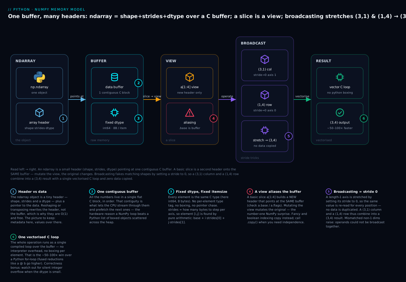
The badges trace the story: the header holds shape, strides and dtype (1) while the values live in one contiguous buffer (2) of a single fixed dtype (3); a basic slice makes a view that aliases that buffer (4); broadcasting stretches a length-1 axis with a stride of 0 so nothing is copied (5); and the whole thing runs as one vectorized C loop (6).
The two workhorse patterns
Ninety percent of real broadcasting is one of two moves: subtracting a per-column statistic from every row, or normalising columns. Both rely on a (3,) row vector broadcasting against a (3, 3) matrix — trailing axis 3 matches 3, and the missing leading axis is treated as 1 and stretched over the rows.
X = np.array([[1., 2., 3.],
              [4., 5., 6.],
              [7., 8., 9.]])

colmean = X.mean(axis=0)      # [4. 5. 6.]   one mean per column, shape (3,)
print(X - colmean)            # (3,3) - (3,) -> broadcast the row over every row
# [[-3. -3. -3.]
#  [ 0.  0.  0.]
#  [ 3.  3.  3.]]
print((X - colmean).mean(axis=0))   # [0. 0. 0.]   columns now centered
Standardising (z-scoring) every column — subtract its mean, divide by its std — is the same pattern twice and is the single most common preprocessing step in machine learning:
Z = (X - X.mean(axis=0)) / X.std(axis=0)
print(np.round(Z.mean(axis=0), 6))   # [-0.  0.  0.]   ~0 (that -0. is machine-precision zero)
print(np.round(Z.std(axis=0), 6))    # [ 1.  1.  1.]   unit variance
Decoding the broadcast ValueError
When shapes don’t line up, NumPy tells you exactly which shapes it couldn’t reconcile. Learn to read it:
A = np.ones((3, 4))
B = np.ones((3,))       # trailing axis 4 vs 3 — neither equal nor 1
A + B
ValueError: operands could not be broadcast together with shapes (3,4) (3,)
The trailing axes are 4 and 3: not equal, neither is 1, so it fails. The fix is to make the vector line up with the axis you actually mean. A (4,) vector broadcasts against (3, 4) fine (it maps to columns). To subtract a per-row value instead, reshape the (3,) into a column (3, 1) with [:, None], so it broadcasts across columns:
v = np.array([1., 2., 3.])
print(X / v[:, None])    # (3,3) / (3,1) — divide each ROW by its own value
# [[1.         2.         3.        ]
#  [2.         2.5        3.        ]
#  [2.33333333 2.66666667 3.        ]]
| Shapes | Result | Why |
|---|---|---|
(3,) and scalar |
(3,) |
Scalar stretches to all |
(3, 4) and (4,) |
(3, 4) |
Trailing 4==4; leading 3 stretches over rows |
(3, 4) and (3,) |
ValueError |
Trailing 4 vs 3: mismatch |
(3, 4) and (3, 1) |
(3, 4) |
(3,1) stretches over columns |
(3, 1) and (1, 4) |
(3, 4) |
Both stretch — outer combination |
(2, 3, 4) and (3, 1) |
(2, 3, 4) |
Align trailing; leading 2 added |
The trick for “which way does my vector go”: v alone (shape (n,)) aligns to the last axis; v[:, None] (shape (n, 1)) aligns to the second-to-last axis. Reshape to steer.
Vectorization: replacing loops with array ops
Vectorization means expressing a computation as whole-array operations so the loop runs in C, not Python. The reflex to build is: whenever you see a for loop doing arithmetic element by element, ask whether an array expression can replace it. A list comprehension is already a big step up from an explicit loop, but NumPy goes further by leaving the interpreter entirely.
Be precise about what vectorization buys you, though: it is a constant-factor win, not an algorithmic-complexity one. Summing a million numbers is O(n) whether you write a Python loop or a.sum() — NumPy just makes each of the n steps ~50-100× cheaper. It will not rescue an O(n²) algorithm from itself; for that you still need the right approach. Vectorization and good complexity are complementary, and the fastest NumPy code has both.
A ReLU (clamp negatives to zero) shows three equivalent vectorized spellings, none with a loop:
v = np.array([-3., -1., 0., 2., 5.])
print(np.where(v > 0, v, 0))   # [0. 0. 0. 2. 5.]   conditional select
print(np.maximum(v, 0))        # [0. 0. 0. 2. 5.]   element-wise max with a scalar
print(v.clip(0, None))         # [0. 0. 0. 2. 5.]   clamp to a range
Reductions and the axis that confuses everyone
A reduction collapses an array to fewer numbers: sum, mean, std, min, max, argmax. With no argument it reduces the whole array to a scalar. With axis=, it reduces along that axis — and this is where nearly everyone gets turned around. The rule that finally makes it stick: axis=k is the axis that disappears. axis=0 collapses the rows, leaving one value per column. axis=1 collapses the columns, leaving one value per row.
M = np.array([[1, 2, 3],
              [4, 5, 6]])          # shape (2, 3)
print(M.sum())            # 21          everything
print(M.sum(axis=0))      # [5 7 9]     collapse rows -> per COLUMN (shape (3,))
print(M.sum(axis=1))      # [ 6 15]     collapse cols -> per ROW    (shape (2,))
print(M.mean(axis=0))     # [2.5 3.5 4.5]
print(M.max(axis=1))      # [3 6]
print(M.argmax(axis=1))   # [2 2]       INDEX of the max in each row
print(M.argmax())         # 5           index into the FLATTENED array
Call on (2, 3) |
Result | Shape | Read as |
|---|---|---|---|
M.sum() |
21 |
scalar | Everything |
M.sum(axis=0) |
[5 7 9] |
(3,) |
Per column (rows collapsed) |
M.sum(axis=1) |
[6 15] |
(2,) |
Per row (columns collapsed) |
M.argmax(axis=1) |
[2 2] |
(2,) |
Winning column index per row |
M.argmax() |
5 |
scalar | Index into the flattened array |
M.sum(axis=1, keepdims=True) |
[[6] [15]] |
(2, 1) |
Keep the axis (for broadcasting back) |
keepdims=True is the quiet hero: it keeps the reduced axis as length 1 so the result broadcasts straight back against the original — exactly what (X - X.mean(axis=0, keepdims=True)) needs when you want to subtract along a specific axis without a manual reshape.
| Reduction | What it gives |
|---|---|
sum / prod |
Total / product |
mean / std / var |
Average / spread |
min / max |
Extremes |
argmin / argmax |
Index of the extreme |
cumsum / cumprod |
Running totals (same shape) |
all / any |
Boolean reductions |
Reshaping and combining arrays
Because shape lives in the header, changing it is usually free (a view). reshape re-lays the same buffer into a new grid; pass -1 for one axis and NumPy solves for it. ravel flattens to 1-D (a view when it can), flatten always copies, and .T transposes by swapping the strides — also a view.
r = np.arange(12)
print(r.reshape(3, 4))       # 3x4 grid, same buffer
print(r.reshape(3, -1))      # -1 -> NumPy infers 4
m = r.reshape(3, 4)
print(m.ravel())             # [ 0  1  2 ... 11]   back to 1-D (a view)
print(m.T.shape)             # (4, 3)              transpose = swapped strides
print(m.reshape(3, 4).base is not None)   # True  reshape returned a VIEW

r.reshape(5, 3)              # 12 elements can't fill 15 slots
ValueError: cannot reshape array of size 12 into shape (5,3)
Because transpose is a view, writing through it writes back to the original — the same aliasing rule as slices:
m = np.arange(6).reshape(2, 3)
m.T[0, 0] = 99
print(m)          # [[99  1  2]
                  #  [ 3  4  5]]   the transpose shares m's buffer
To join arrays, concatenate glues along an existing axis, while stack creates a new axis. vstack/hstack are the common 2-D shortcuts.
a = np.array([[1, 2], [3, 4]])
b = np.array([[5, 6], [7, 8]])
print(np.concatenate([a, b], axis=0))   # stack rows -> (4, 2)
print(np.concatenate([a, b], axis=1))   # glue columns -> (2, 4)
print(np.vstack([a, b]))                 # same as axis=0
print(np.hstack([a, b]))                 # same as axis=1

x = np.array([1, 2, 3]); y = np.array([4, 5, 6])
print(np.stack([x, y]))          # NEW axis -> shape (2, 3): [[1 2 3] [4 5 6]]
print(np.stack([x, y], axis=1))  # [[1 4] [2 5] [3 6]]   shape (3, 2)
| Operation | Does | View/copy | Note |
|---|---|---|---|
a.reshape(r, c) |
Re-lay same data | View if contiguous | -1 infers one axis |
a.ravel() |
Flatten to 1-D | View when possible | Fast |
a.flatten() |
Flatten to 1-D | Always a copy | Safe to mutate |
a.T / a.transpose() |
Swap axes | View | Strides swapped |
np.concatenate([...], axis) |
Join on existing axis | Copy | Shapes must match off-axis |
np.stack([...], axis) |
Join on a new axis | Copy | Inputs must be same shape |
np.vstack / np.hstack |
Row-wise / col-wise join | Copy | 2-D convenience |
dtypes and the pitfalls that bite
The fixed-dtype buffer that makes NumPy fast also makes it capable of quietly wrong answers. These four pitfalls account for most “the math is subtly off” bug reports.
Silent integer overflow
An int8 holds values from -128 to 127. Push past the top and it wraps around to the bottom — modular arithmetic, exactly like C, with no exception on array operations. This is not a hypothetical; it happens the moment you pick a small dtype to save memory and your data grows.
x = np.array([127], dtype=np.int8)
print(x + 1)                     # [-128]   wrapped! 127 + 1 rolled over
print((x + 1).dtype)             # int8     stays int8 (NumPy 2.x, NEP 50)

y = np.array([100, 100], dtype=np.int8)
print(y + y)                     # [-56 -56]   200 wrapped to -56, NO warning
print(np.iinfo(np.int8).min, np.iinfo(np.int8).max)   # -128 127

z = np.array([200], dtype=np.uint8)
print(z + np.uint8(100))         # [44]    uint8 is 0-255; 300 mod 256 = 44
Two things make this dangerous. First, array operations wrap silently — no warning at all (only scalar NumPy operations emit RuntimeWarning: overflow encountered). Second, in NumPy 2.0+, adding a Python int to an int8 array keeps it int8 (the NEP 50 promotion rules), so x + 1 overflows rather than promoting to a wider type. The fix is to choose a dtype with headroom, or cast up before the risky operation: x.astype(np.int64) + 1. When you iinfo your dtype and your data approaches those bounds, widen it.
| dtype | Min | Max | Overflow example |
|---|---|---|---|
int8 |
-128 | 127 | 127 + 1 → -128 |
uint8 |
0 | 255 | 255 + 1 → 0; 200 + 100 → 44 |
int16 |
-32,768 | 32,767 | Common for audio |
int32 |
~-2.1×10⁹ | ~2.1×10⁹ | Watch large sums |
int64 |
~-9.2×10¹⁸ | ~9.2×10¹⁸ | Effectively safe for counts |
Read your dtype’s exact bounds at runtime with np.iinfo(np.int8) (integers) or np.finfo(np.float32) (floats). If a running total might approach the ceiling, do the arithmetic in int64.
Version note: pre-2.0 NumPy sometimes promoted
int8 + python_intto a larger dtype, hiding the overflow. NumPy 2.x (NEP 50) makes the Python scalar “weak,” so the array’sint8wins and the wrap is visible. This lesson targets NumPy 2.x on Python 3.12; check withnp.__version__.
Int vs float division, and casting
/ (true division) always produces float64; // (floor division) stays integer. Casting a float array to int with .astype() truncates toward zero — it does not round — so -1.9 becomes -1, not -2. Round first if you mean to round.
print(np.array([7, 8]) / 2)      # [3.5 4. ]   float64 always
print(np.array([7, 8]) // 2)     # [3 4]       stays int64
print(np.array([1.9, 2.1, -1.9]).astype(int))          # [ 1  2 -1]   truncates!
print(np.round([1.9, 2.1, -1.9]).astype(int))          # [ 2  2 -2]   round first
nan poisons everything
nan (“not a number”) is a special float that represents missing or undefined data. Its defining, disorienting property: nan is not equal to anything, including itself. And it propagates — any ordinary arithmetic or reduction touching a nan yields nan, so one missing value silently turns your whole mean into nan.
a = np.array([1.0, 2.0, np.nan, 4.0])
print(a.mean())          # nan          one nan poisons the mean
print(np.nan == np.nan)  # False        the classic surprise
print(np.isnan(a))       # [False False  True False]   how to FIND nans
print(np.nanmean(a))     # 2.3333333333333335   nan-skipping mean
print(np.nansum(a))      # 7.0
You can never test for nan with ==; use np.isnan(). And to reduce data that contains missing values, reach for the nan-aware reductions: nanmean, nansum, nanstd, nanmax, and friends, which skip the nans instead of propagating them.
Float equality — use isclose, never ==
Because floats are binary approximations, 0.1 + 0.2 is not exactly 0.3, so == on floats is a coin-flip. Never compare floats with ==. Use np.isclose for scalars/arrays and np.allclose to ask “are these two arrays equal within tolerance?”
print(0.1 + 0.2 == 0.3)                     # False   the famous float gotcha
print(np.isclose(0.1 + 0.2, 0.3))           # True    within tolerance
u = np.array([0.1 + 0.2, 1.0]); w = np.array([0.3, 1.0])
print(np.array_equal(u, w))                 # False   exact — fails
print(np.allclose(u, w))                    # True    tolerant — the right test
| Pitfall | Symptom | Fix |
|---|---|---|
| Integer overflow | Values wrap negative/small | Widen dtype: .astype(np.int64); check np.iinfo |
astype(int) truncates |
-1.9 → -1 not -2 |
np.round(x).astype(int) |
nan in a reduction |
mean() returns nan |
np.nanmean, np.nansum; find with np.isnan |
nan == nan |
Always False |
np.isnan(x), never == np.nan |
Float == |
Equal-looking values compare unequal | np.isclose / np.allclose |
Basic linear algebra
NumPy started life as a numerical-linear-algebra library, and the essentials are a few operators away. The one distinction to burn in: * is element-wise, @ is matrix multiplication. They are completely different operations that happen to share operands.
P = np.array([[1, 2], [3, 4]])
print(P * P)    # [[ 1  4]     element-wise: each cell squared
                #  [ 9 16]]
print(P @ P)    # [[ 7 10]     matrix product: rows-times-columns
                #  [15 22]]
This is the single most common source of “my matrix math is wrong” — A * B looks like multiplication but multiplies cell-by-cell, requiring matching shapes (or broadcasting), while A @ B is the real matrix product with the rows-times-columns rule and the inner dimensions must agree.
| Expression | Operation | Result (2-D) | Shape rule |
|---|---|---|---|
A * B |
Element-wise product | Cell-by-cell | Same shape / broadcastable |
np.multiply(A, B) |
Element-wise product | Same as * |
Same shape / broadcastable |
A @ B |
Matrix product | Rows × columns | A.shape[1] == B.shape[0] |
np.matmul(A, B) |
Matrix product | Same as @ |
Batched for >2-D |
np.dot(A, B) |
Matrix product (2-D) | Same as @ |
Inner dims agree |
a @ b (both 1-D) |
Dot product | Scalar | Same length |
@ is the modern operator (Python 3.5+); np.dot and np.matmul do the same for 2-D arrays. For 1-D arrays, a @ b is the dot product (a scalar).
A = np.array([[2., 1.], [1., 3.]])
b = np.array([1., 2.])
print(A @ A)              # [[ 5.  5.] [ 5. 10.]]   matrix product
print(np.dot(b, b))      # 5.0                     dot product -> scalar
The high-value tools live in np.linalg. To solve a linear system Ax = b, use np.linalg.solve — never compute the inverse and multiply, which is slower and less numerically stable. norm gives vector length; inv inverts; det is the determinant; eye is the identity.
A = np.array([[2., 1.], [1., 3.]])
b = np.array([1., 2.])
x = np.linalg.solve(A, b)     # solve A x = b
print(x)                      # [0.2 0.6]
print(np.allclose(A @ x, b))  # True     verify with allclose, not ==

print(np.linalg.inv(A))       # [[ 0.6 -0.2] [-0.2  0.4]]
print(np.linalg.norm(b))      # 2.23606797749979    sqrt(1^2 + 2^2)
print(np.linalg.det(A))       # 5.000000000000001   ~5 (float noise)
A singular (non-invertible) matrix raises rather than returning garbage — a friendly failure:
np.linalg.inv(np.array([[1., 2.], [2., 4.]])) # rows are proportional
numpy.linalg.LinAlgError: Singular matrix
| Operation | Call | Returns |
|---|---|---|
| Element-wise product | A * B |
Same shape |
| Matrix product | A @ B, np.matmul, np.dot |
Matrix |
| Dot product (1-D) | a @ b, np.dot(a, b) |
Scalar |
| Transpose | A.T |
View |
| Identity | np.eye(n) |
n×n |
Solve Ax=b |
np.linalg.solve(A, b) |
x (preferred over inv) |
| Inverse | np.linalg.inv(A) |
A⁻¹ (raises if singular) |
| Determinant | np.linalg.det(A) |
Scalar |
| Norm (length) | np.linalg.norm(v) |
Scalar |
| Eigenvalues | np.linalg.eig(A) |
(values, vectors) |
Hands-on lab
This lab exercises every idea above on real arrays. NumPy is a third-party package, so work inside a virtual environment — never pip install into system Python.
⚠️ Use a Python 3.12+ interpreter (macOS system Python is 3.9). Create and activate the venv, then install NumPy:
python3.12 -m venv .venv
source .venv/bin/activate        # Windows: .venv\Scripts\activate
pip install numpy
python -c "import numpy as np; print(np.__version__)"   # 2.5.1 (or later)
Create numpy_lab.py and add each step, running python numpy_lab.py as you go. Every output is exact except the timings in Step 6, which depend on your machine.
Step 1 — Create arrays and read the header.
import numpy as np

rng  = np.random.default_rng(7)
a    = np.arange(12).reshape(3, 4)
z    = np.zeros((2, 3))
grid = np.linspace(0, 1, 5)
r    = rng.integers(0, 100, size=6)

print(a)
# [[ 0  1  2  3]
#  [ 4  5  6  7]
#  [ 8  9 10 11]]
print("shape", a.shape, "| ndim", a.ndim, "| dtype", a.dtype,
      "| itemsize", a.itemsize, "| strides", a.strides)
# shape (3, 4) | ndim 2 | dtype int64 | itemsize 8 | strides (32, 8)
print("z.dtype", z.dtype, "| grid", grid, "| r", r)
# z.dtype float64 | grid [0.   0.25 0.5  0.75 1.  ] | r [94 62 68 89 57 77]
What just happened: strides (32, 8) says stepping one row jumps 32 bytes (four int64s = one row) and one column jumps 8 — the header mapping the flat buffer onto a 3×4 grid. The seeded rng makes r reproducible.
Step 2 — Prove the view-vs-copy aliasing, then fix it.
base = np.array([10, 20, 30, 40, 50])
view = base[1:4]              # a VIEW
view[0] = 999                 # write through the view
print("base:", base)          # base: [ 10 999  30  40  50]   <- ORIGINAL changed!
print("view.base is base:", view.base is base)   # True

safe = base[1:4].copy()       # an independent COPY
safe[0] = -7
print("base:", base, "| safe:", safe)  # base: [ 10 999  30  40  50] | safe: [-7 30 40]
print("safe.base is None:", safe.base is None)   # True
What just happened: mutating view reached back and changed base, because a basic slice shares the buffer. .copy() broke the link — safe owns its data (base is None), so writing to it left base alone. This is the number-one NumPy surprise, proven in eight lines.
Step 3 — Broadcast-normalise a matrix column-wise.
rng3 = np.random.default_rng(3)
X    = rng3.normal(loc=[10, 100, 1000], scale=[1, 20, 5], size=(5, 3))
mu   = X.mean(axis=0)         # per-column mean, shape (3,)
sd   = X.std(axis=0)          # per-column std,  shape (3,)
Z    = (X - mu) / sd          # (5,3) - (3,) / (3,)  -> broadcast over rows

print("X.mean(axis=0):", np.round(mu, 3))   # [ 10.499  85.27  997.93 ]
print("X.std(axis=0) :", np.round(sd, 3))   # [ 1.921 19.132  2.598]
print("Z.mean(axis=0):", np.round(Z.mean(axis=0), 6))  # [-0.  0.  0.]
print("Z.std(axis=0) :", np.round(Z.std(axis=0), 6))   # [1. 1. 1.]
What just happened: the three columns started on wildly different scales (means ~10, ~85, ~998). One broadcast expression centered and scaled every column to mean 0, std 1 — no loop, no per-column code. This is the standardisation step at the front of nearly every ML pipeline.
Step 4 — Mask and np.where.
rng4  = np.random.default_rng(2)
temps = rng4.normal(30, 8, size=12).round(1)
print("temps      :", temps)
# [31.5 25.8 26.7 10.5 44.4 39.2 27.4 36.2 32.2 25.6 37.8 27.5]
print("hot (>35)  :", temps[temps > 35])       # [44.4 39.2 36.2 37.8]
print("count hot  :", (temps > 35).sum())      # 4
print("flagged    :", np.where(temps > 35, temps, 0.0))
# [ 0.   0.   0.   0.  44.4 39.2  0.  36.2  0.   0.  37.8  0. ]
print("hot indices:", np.where(temps > 35)[0]) # [ 4  5  7 10]
What just happened: the mask temps > 35 selected the hot days, .sum() counted them, np.where(cond, temps, 0) zeroed the rest, and np.where(cond) returned their positions — four different questions answered with no loop.
Step 5 — Reduce along axis=0 vs axis=1.
sales = np.array([[10, 20, 30, 40],
                  [50, 15, 25, 35],
                  [ 2,  4, 60,  8]])
print("per-column total (axis=0):", sales.sum(axis=0))    # [ 62  39 115  83]
print("per-row total    (axis=1):", sales.sum(axis=1))    # [100 125  74]
print("best column each row     :", sales.argmax(axis=1)) # [3 0 2]
What just happened: axis=0 collapsed the three rows into one total per column; axis=1 collapsed the four columns into one total per row. argmax(axis=1) found each row’s peak column — row 0 peaks at index 3, row 1 at index 0, row 2 at index 2. Remember: the axis you name is the axis that disappears.
Step 6 — MEASURE vectorised vs a Python loop on 1M elements.
import time

N  = 1_000_000
xs = list(range(N)); ys = list(range(N))

t0 = time.perf_counter()
out = [0] * N
for i in range(N):
    out[i] = xs[i] + ys[i]
t_loop = time.perf_counter() - t0

xa = np.arange(N); ya = np.arange(N)
t0 = time.perf_counter()
outa = xa + ya
t_np = time.perf_counter() - t0

print(f"python loop : {t_loop*1000:8.2f} ms")   # python loop :    84.69 ms
print(f"numpy xa+ya : {t_np*1000:8.3f} ms")      # numpy xa+ya :     1.000 ms
print(f"speedup     : {t_loop/t_np:8.0f}x")      # speedup     :       85x
What just happened: the same element-wise add ran ~85× faster as one array expression than as a hand-written loop (across runs I saw 54×–91×; the exact figure wobbles with system load, the order of magnitude does not). The loop pays Python’s per-element interpreter and boxing tax a million times; xa + ya pays it zero times.
Step 7 — Reproduce an int8 overflow.
small = np.array([100, 120, 127], dtype=np.int8)
print("small        :", small, small.dtype)          # [100 120 127] int8
print("small + 10   :", small + np.int8(10))         # [ 110 -126 -119]  <- wrapped!
print("int8 max/min :", np.iinfo(np.int8).max, np.iinfo(np.int8).min)  # 127 -128
big = small.astype(np.int64) + 10
print("as int64 + 10:", big, big.dtype)              # [110 130 137] int64  <- no wrap
What just happened: 120 + 10 and 127 + 10 sailed past the int8 ceiling of 127 and wrapped to negatives — silently, no error. Casting to int64 first gave the honest answer. Any time you pick a narrow dtype to save memory, this is the risk you accept.
You have now, on real arrays, inspected the header, proven view-vs-copy aliasing and fixed it, broadcast-normalised a matrix, masked with np.where, reduced along both axes, measured the vectorization win, and reproduced a silent overflow — every core idea of the lesson.
Common mistakes and troubleshooting
| Symptom / traceback | Cause | Fix |
|---|---|---|
| “My original array changed and I never touched it” | A basic slice is a view; you mutated it | Take a[1:4].copy() when you need independence. Diagnose with .base / .flags['OWNDATA'] |
ValueError: operands could not be broadcast together with shapes (3,4) (3,) |
Trailing axes aren’t equal and neither is 1 | Align shapes: use a (4,) vector, or reshape to (3, 1) with [:, None] to broadcast the other way |
ValueError: The truth value of an array ... is ambiguous. Use a.any() or a.all() |
Used and/or/if on a boolean array |
Combine masks with &/|/~; wrap each comparison: (a > 2) & (a < 7) |
(a > 2) & a < 7 returns a wrong-but-valid array |
& binds tighter than <; missing parentheses |
Parenthesise every comparison: (a > 2) & (a < 7) |
mean() / sum() returns nan |
A nan propagated through the reduction |
Use np.nanmean / np.nansum; locate them with np.isnan(a) |
Testing x == np.nan is always False |
nan never equals anything, even itself |
Use np.isnan(x) |
| Two equal-looking float arrays compare unequal | Floating-point rounding; == is exact |
np.isclose(a, b) / np.allclose(a, b) |
| Integer results wrap to negative/tiny values | Silent overflow of a small dtype (int8/uint8) |
Widen: a.astype(np.int64); check bounds with np.iinfo(a.dtype) |
ValueError: cannot reshape array of size 12 into shape (5,3) |
New shape’s product ≠ element count | Ensure rows*cols == a.size; use -1 to infer one axis |
TypeError: only integer scalar arrays can be converted... or list+array oddities |
Mixed a Python list and an ndarray expecting element-wise math |
np.array(list) first; remember list + list concatenates, array + array adds |
numpy.linalg.LinAlgError: Singular matrix |
Inverting/solving a non-invertible matrix | Check np.linalg.det(A); use np.linalg.lstsq for least-squares |
In-place op a += b raises “could not be broadcast” |
The broadcast result is bigger than a |
You can’t broadcast into a smaller array; assign to a new one or resize a |
astype(int) gives -1 from -1.9 |
Casting truncates toward zero, doesn’t round | np.round(x).astype(int) |
Three of these swallow the most hours, so they get extra words.
1. The view aliasing surprise. When an array changes “by itself,” look upstream for a basic slice or transpose you thought was a copy — sub = big[10:20], col = m[:, 0], t = m.T. All three are live views; writing to them writes to the parent, and passing one into a function that mutates it mutates your original. The diagnostic is x.base is None (owns its data → safe) versus x.base is parent (a view → shared). The fix is a deliberate .copy() at the boundary. Fancy and boolean indexing don’t have this problem — they always copy — which is why big[big > 0] is safe to mutate but big[10:20] is not.
2. Broadcasting failures and, worse, broadcasting successes you didn’t intend. The error message is the easy case — it prints both shapes and you fix the mismatch. The insidious case is when two arrays broadcast accidentally: a (1000,) and a (1000, 1) combine into a (1000, 1000) array — a million elements from two thousand — and you get a memory blow-up or nonsense means, with no error at all. When a result has a surprising shape, print .shape on both operands before the operation. A stray [:, None] or a missing .ravel() is usually the culprit.
3. Silent integer overflow. This one produces wrong numbers, not a traceback, so it hides. It appears when you pick int8/int16/uint8 to save memory (image pixels are the classic uint8 case) and then sum or scale them. np.array([200, 100], dtype=np.uint8).sum() is not 300. The habit that saves you: do arithmetic in int64 or float64, and only narrow the dtype for storage, after the math is done. When in doubt, a.astype(np.int64) before the risky step and check your dtype’s ceiling with np.iinfo.
Cheat-sheet
| Syntax | What it does |
|---|---|
np.array([...]) |
Build an array from a list/tuple |
np.zeros(s) / np.ones(s) / np.full(s, v) |
Filled arrays |
np.arange(a, b, step) |
Range as array (b excluded) |
np.linspace(a, b, n) |
n points a…b (b included) |
np.eye(n) |
n×n identity |
rng = np.random.default_rng(seed) |
Seeded random Generator (modern API) |
rng.random(s) / rng.integers(lo, hi, s) / rng.normal(m, sd, s) |
Random arrays |
a.shape / a.ndim / a.dtype / a.size |
The header: grid / axes / type / count |
a.strides / a.itemsize / a.nbytes |
Bytes per axis step / per item / total |
a[i, j] |
Index a 2-D array (tuple index) |
a[1:3, :2] |
Slice — returns a VIEW |
a.copy() |
Independent copy (owns its buffer) |
a.base is None / a.flags['OWNDATA'] |
Is it a view or does it own data? |
a[a > 0] |
Boolean mask — returns a COPY |
a[[0, 2, 4]] |
Fancy index — returns a COPY |
a[mask] = v |
Masked assignment — writes in place |
(a > 2) & (a < 7) |
Combine masks (& | ~, parenthesise!) |
np.where(cond, x, y) |
Element-wise ternary select |
np.where(cond) |
Indices where True |
a + b, a * b |
Element-wise ops (broadcasting) |
a @ b |
Matrix multiply / dot product |
a.sum(axis=0) |
Per-column (rows collapse) |
a.sum(axis=1) |
Per-row (columns collapse) |
a.mean/std/min/max/argmax(axis=) |
Reductions along an axis |
a.sum(axis=1, keepdims=True) |
Keep axis for broadcasting back |
a.reshape(r, c) / a.reshape(-1) |
Reshape (view); -1 infers an axis |
a.ravel() (view) / a.flatten() (copy) |
Flatten to 1-D |
a.T |
Transpose (view — swapped strides) |
np.concatenate([a, b], axis) |
Join on an existing axis |
np.stack([a, b], axis) |
Join on a new axis |
np.vstack / np.hstack |
Row-wise / column-wise join |
a.astype(np.int64) |
Cast dtype (truncates float→int) |
np.iinfo(dt) / np.finfo(dt) |
Integer / float dtype limits |
np.isnan(a) / np.nanmean(a) |
Find / skip nans |
np.isclose(a, b) / np.allclose(a, b) |
Float equality with tolerance |
np.linalg.solve(A, b) |
Solve Ax = b (preferred over inv) |
np.linalg.inv/det/norm(...) |
Inverse / determinant / norm |
Interview and exam questions
Q: Why is a NumPy array so much faster than a Python list for numeric work?
A: A list holds pointers to boxed Python objects scattered on the heap; every element operation costs a type check, an unbox, the math, a rebox, and a pointer store, all in the interpreter. An ndarray stores one fixed C type packed in a single contiguous buffer, so NumPy runs the whole operation as one compiled C loop with no per-element boxing and no interpreter overhead — typically ~50-100× faster on bulk element-wise work, and more on fused reductions. The trade is rigidity: fixed dtype, hence silent overflow.
Q: What are shape and strides, and why are reshape and transpose “free”?
A: shape is the length along each axis; strides is the number of bytes to step to the next element along each axis. NumPy locates element [i, j] by arithmetic: base + i*strides[0] + j*strides[1]. Reshape and transpose just hand you a new header (new shape/strides) pointing at the same buffer — no data moves — which is why they’re O(1) and return views.
Q: When does a slice return a view versus a copy, and why does it matter?
A: Basic slicing (a[1:4], a[:, 0], a.T) returns a view onto the same buffer, so mutating it mutates the original. Advanced indexing — fancy (integer arrays) and boolean masks — returns a copy, because the selected elements aren’t regularly strided so no header could describe them. It matters because writing through a view you thought was a copy is the most common NumPy bug. Diagnose with a.base / a.flags['OWNDATA']; force a copy with .copy().
Q: State the broadcasting rule. What do (3, 1) and (1, 4) produce?
A: Compare shapes from the trailing axis backward; each axis pair must be equal or have one side equal to 1, in which case that side is stretched (stride set to 0, no copy). (3, 1) and (1, 4): trailing 1 vs 4 → stretch to 4; next 3 vs 1 → stretch to 3; result (3, 4) — an outer combination. Mismatched non-1 axes raise ValueError: operands could not be broadcast together.
Q: You have a (100, 3) matrix X. Write z-score normalisation per column.
A: Z = (X - X.mean(axis=0)) / X.std(axis=0). X.mean(axis=0) and X.std(axis=0) are shape (3,); they broadcast against every one of the 100 rows. Result: each column has mean ~0 and std 1. Use keepdims=True if you’d rather keep the (1, 3) shape explicit.
Q: What’s the difference between axis=0 and axis=1 in a reduction?
A: The named axis is the one that collapses. On a 2-D array, axis=0 collapses the rows and returns one value per column; axis=1 collapses the columns and returns one value per row. So on a (2, 3) array, sum(axis=0) has shape (3,) and sum(axis=1) has shape (2,).
Q: Why does a > 2 and a < 7 raise, and what’s correct?
A: and forces Python to evaluate the truth of a whole boolean array, which is ambiguous — hence ValueError: The truth value of an array with more than one element is ambiguous. Use the element-wise bitwise operators with parentheses: (a > 2) & (a < 7). Parentheses are mandatory because & binds tighter than the comparison operators; without them (a > 2) & a < 7 silently computes something else entirely.
Q: Demonstrate silent integer overflow and explain the NumPy 2.x behaviour.
A: np.array([127], dtype=np.int8) + 1 gives [-128] — it wraps past the int8 ceiling of 127 with no error on array operations. In NumPy 2.0+ (NEP 50), the Python int 1 is “weak” and takes the array’s int8 dtype rather than promoting to a wider type, so the overflow is visible. Fix by widening first: a.astype(np.int64) + 1. Check limits with np.iinfo(np.int8).
Q: How do you compare floats for equality, and why not ==?
A: Floats are binary approximations, so 0.1 + 0.2 == 0.3 is False. Use np.isclose(a, b) for element-wise tolerance, or np.allclose(a, b) to ask whether two whole arrays match within tolerance. Never gate logic on exact float ==.
Q: How do you handle nan in a dataset?
A: nan propagates — one nan makes an entire mean()/sum() return nan — and it’s never equal to anything, so you can’t test it with ==. Locate nans with np.isnan(a), and reduce with the nan-aware functions np.nanmean, np.nansum, np.nanstd, which skip them.
Q (coding): Given a = np.arange(1, 21), return the even numbers greater than 10, then replace all odd numbers with -1.
A: a[(a > 10) & (a % 2 == 0)] → [12 14 16 18 20]. Then np.where(a % 2 == 1, -1, a) builds a new array with odds set to -1; or a[a % 2 == 1] = -1 to modify in place. Note the parentheses around each mask.
Q (coding): Solve the system 2x + y = 1, x + 3y = 2 without inverting a matrix.
A: A = np.array([[2., 1.], [1., 3.]]); b = np.array([1., 2.]); x = np.linalg.solve(A, b) → [0.2 0.6]. Verify with np.allclose(A @ x, b). Prefer solve over inv(A) @ b — it’s faster and numerically more stable.
Key takeaways
- The
ndarrayis one contiguous, fixed-dtype C buffer plus a header (shape,strides,dtype). That layout is why NumPy runs vectorized operations as compiled C loops — ~50-100× faster than a Python loop on bulk work — and why reshape/transpose are free (they only rewrite the header). - Vectorize: replace element-by-element
forloops with whole-array expressions. The loop pays Python’s boxing and interpreter tax per element;a + bpays it never. Measure it once and you’ll never write the loop again. - A basic slice is a VIEW, not a copy — it aliases the same buffer, so mutating it mutates the original. Fancy and boolean indexing return copies. Use
.copy()for independence and.base/.flagsto tell which you have. - Broadcasting aligns shapes from the trailing axis; a size-1 axis stretches (stride 0, no copy). It turns “subtract the column means” and “z-score each column” into one-liners. Read the
ValueError— it prints both shapes. - Reduce along the axis that disappears:
axis=0gives per-column results,axis=1per-row. Combine boolean masks with&/|/~and parenthesise every comparison —and/orraise the “ambiguous truth value” error. - The fixed dtype cuts both ways: integer overflow wraps silently (do math in
int64/float64, narrow only for storage),astype(int)truncates,nanpoisons reductions (usenp.nanmean, find withnp.isnan), and float==is unreliable (usenp.isclose). - Linear algebra is a few calls away:
*is element-wise,@is matrix multiply;np.linalg.solve(A, b)beats inverting;norm,inv,det,eyecover the basics — and a singular matrix raisesLinAlgErrorrather than lying.