Every data job — cleaning a messy export, joining two systems, computing a metric, prepping features for a model — starts by getting a table into memory and slicing it up. Python’s list and dict are wonderful for scalars and records, but the moment your data is tabular and labelled — rows of things, each with named columns, some numbers, some text, some dates, some missing — you want a tool built for exactly that shape. That tool is pandas.
The one-line pitch: pandas is a spreadsheet you can program. A DataFrame is a sheet of rows and columns, but instead of clicking cells you write expressions — filter, transform, aggregate, join — and they run on millions of rows in vectorised C, not a Python loop. It is the single most-used library in data science, and it is built directly on top of NumPy: every column is a NumPy array wearing a label. If you have met NumPy’s arrays and vectorised math elsewhere in this course, pandas is what happens when you give those arrays names and let columns of different types live side by side.
This is Part 1 of two. Here we build the mental model — the Series, the DataFrame, the all-important index — and then spend most of the lesson on selection: the [] / .loc / .iloc distinction, boolean filtering, and the notorious SettingWithCopyWarning. Part 2 picks up groupby, merge/join, reshaping, and the full treatment of missing data. Get this lesson solid and Part 2 is downhill.
Everything below was executed on Python 3.12.3 with pandas 3.0.3. Pandas 3.0 changed several defaults you will see in the output (a real
strdtype for text, microseconddatetime64[us], Copy-on-Write on by default). Where the behaviour differs from older pandas, there is a version note — because you will meet both.
Why this matters
Picture a CSV of employees: a name, a department, an age, a salary, a hire date, whether they work remotely. In plain Python you would reach for a list of dicts — [{"name": "Ana", "age": 37, ...}, ...]. That works until you want to do something: “average salary per department”, “everyone over 30 in Engineering”, “give the Sales team a 10% raise”. Each of those becomes a hand-rolled loop, a running total, an if, an accumulator. Twenty lines, a bug or two, and it crawls on a million rows.
Pandas turns each of those into one line that reads like the question — df.groupby("department")["salary"].mean() — and runs at C speed. The reason it can is the whole point of this lesson: pandas stores each column as a single typed array (a NumPy array underneath), so “add 10% to every salary” is one vectorised multiply, not a million Python iterations. The table below is the shift in thinking:
| Task | Plain Python (list of dicts) | Pandas |
|---|---|---|
| Load a CSV | csv.DictReader, manual type conversion |
pd.read_csv("f.csv") — one call, types inferred |
| Everyone over 30 | [r for r in rows if r["age"] > 30] |
df[df["age"] > 30] |
| Average salary | loop, sum, divide, guard empty | df["salary"].mean() |
| Per-department average | nested dict accumulator | df.groupby("dept")["salary"].mean() |
| 10% raise for Sales | loop with an if |
df.loc[df.dept == "Sales", "salary"] *= 1.1 |
| Speed on 1M rows | seconds, pure-Python | milliseconds, vectorised |
The catch — and the reason this lesson is long — is that pandas’ power comes from one idea that trips up every beginner: the index. A pandas object is not just data; it is data plus a set of labels glued to it, and those labels drive alignment, selection, and assignment. Master the index and pandas feels like magic. Ignore it and you will fight SettingWithCopyWarning, mysterious NaNs, and KeyErrors for months. So we start with the smallest object that has an index — the Series — and build up.
The Series: a 1-D array with an index
A Series is a one-dimensional labelled array: a column of values, plus an index of labels, plus a dtype. Think of it as the love-child of a NumPy array (the values, all one type, fast) and a dict (the labels, for lookup by name).
import pandas as pd

temps = pd.Series([19.5, 22.0, 25.3, 21.8],
                  index=["Mon", "Tue", "Wed", "Thu"],
                  name="temp_c")
print(temps)
Mon    19.5
Tue    22.0
Wed    25.3
Thu    21.8
Name: temp_c, dtype: float64
Read that output carefully — it is the whole anatomy of a Series. The left column is the index (Mon…Thu), the right column is the values, the name is the Series’ own label (it becomes a column name inside a DataFrame), and dtype: float64 says every value is a 64-bit float, stored as a contiguous NumPy array. You look things up by label, and the values travel as one array:
print(temps["Wed"])       # => 25.3          (lookup by label, like a dict)
print(temps.values)       # => [19.5 22.  25.3 21.8]   (a NumPy ndarray)
print(list(temps.index))  # => ['Mon', 'Tue', 'Wed', 'Thu']
If you leave the index off, pandas gives you a default RangeIndex (0, 1, 2, …) — which is why a plain Series looks like a list. But the index is always there, and it is the difference between a Series and a NumPy array.
There are several ways to build a Series; you will meet all of them:
| How | Example | Index you get |
|---|---|---|
| From a list | pd.Series([10, 20, 30]) |
Default RangeIndex 0,1,2 |
| List + index | pd.Series([10, 20], index=["a", "b"]) |
Your labels a, b |
| From a dict | pd.Series({"a": 10, "b": 20}) |
Keys become the index |
| Scalar + index | pd.Series(0, index=["a", "b", "c"]) |
Broadcast: every label gets 0 |
| From a NumPy array | pd.Series(np.arange(5)) |
Default RangeIndex |
The index is the superpower: automatic alignment
Here is the single most important behaviour in pandas, and it lives in the Series. When you combine two Series, pandas aligns them by label, not by position:
a = pd.Series({"eng": 10, "sales": 5, "support": 3})
b = pd.Series({"sales": 2, "eng": 4, "marketing": 9})
print(a + b)
eng          14.0
marketing     NaN
sales         7.0
support       NaN
dtype: float64
Look at what happened. eng added to eng (10 + 4 = 14) and sales to sales (5 + 2 = 7) even though they were in a different order in the two Series. Labels only in one side — marketing, support — produced NaN (“not a number”, pandas’ missing marker), because there was nothing to add them to. A NumPy array would have added position-by-position and given you nonsense; pandas added by meaning. This is why the index is not decoration — it is the join key that makes every pandas operation line up correctly. Hold onto that; it explains half the surprises later in this lesson.
A Series sits between the two Python containers you already know:
list |
dict |
pd.Series |
|
|---|---|---|---|
| Access by | position x[0] |
key d["a"] |
both — s.iloc[0] and s["a"] |
| Values are | any mix | any mix | one dtype (fast, NumPy-backed) |
| Ordered? | yes | yes (insertion) | yes |
| Vectorised math | no (loop) | no | yes — s * 2, s > 30 |
| Aligns on combine | no | no | yes, by label |
The DataFrame: an ordered dict of Series on one shared index
Stack several Series side by side, all sharing one common index, and you have a DataFrame — the two-dimensional table that is pandas’ headline object. The mental model to burn in: a DataFrame is an ordered dict of Series, where every Series (column) is aligned on the same row index.
df = pd.DataFrame({
    "name": ["Ana", "Bao", "Chidi"],
    "age":  [37, 29, 41],
    "dept": ["Engineering", "Engineering", "Sales"],
})
print(df)
print(df.dtypes)
    name  age         dept
0    Ana   37  Engineering
1    Bao   29  Engineering
2  Chidi   41        Sales

name      str
age     int64
dept      str
dtype: object
Each key became a column; the values became that column’s Series; and because we gave no index, all three columns share a default RangeIndex 0,1,2 down the left. Crucially, each column keeps its own dtype — age is int64, name and dept are str. A DataFrame is heterogeneous across columns but homogeneous within each column, which is exactly what a real table needs.
pandas 3.0 note: text columns now report dtype
str, a real string type. On pandas 2.x and earlier the same columns showobject(Python objects in a box). You will seeobjectconstantly in older tutorials and Stack Overflow answers — it means the same “this column holds strings”, just slower and less type-safe. A genuinely mixed column (say strings and ints together) is stillobjecton every version.
There are three common ways real data arrives as a DataFrame:
| Source | Code | When |
|---|---|---|
| Dict of columns | pd.DataFrame({"a": [1,2], "b": [3,4]}) |
You have data column-wise |
| List of row-dicts | pd.DataFrame([{"a":1,"b":3}, {"a":2,"b":4}]) |
Records from an API/JSON |
| NumPy 2-D array | pd.DataFrame(arr, columns=[...], index=[...]) |
Numeric matrix, add labels |
The list-of-dicts form is worth a close look because it shows the index doing its job on columns:
recs = [{"name": "Ana", "age": 37},
        {"name": "Bao", "age": 29, "remote": True}]
print(pd.DataFrame(recs))
  name  age remote
0  Ana   37    NaN
1  Bao   29   True
The first record has no remote key, so pandas aligned the columns by name and filled the hole with NaN — the same label-alignment you saw with Series, now across records. This is why JSON from a web API, where records have ragged keys, loads cleanly: pandas unions the keys into columns and fills the gaps.
Loading real data: read_csv, done properly
You rarely type data in; you load it. pd.read_csv is the workhorse, and 90% of pandas bugs are really read_csv bugs — a numeric ID read as text, a date left as a string, a wrong-type column — that quietly poison every later step. So load deliberately, then inspect immediately.
For the whole lesson we use one small, realistic dataset. Create it now with a plain file write (this is exactly what the lab does):
import csv
rows = [
    ("emp_id","name","department","city","age","salary","hire_date","remote","manager_id"),
    (1,"Ana Garcia","Engineering","Madrid",37,98000,"2018-03-11","True",""),
    (2,"Bao Nguyen","Engineering","Singapore",29,88000,"2021-07-01","True",1),
    (3,"Chidi Okafor","Sales","Lagos",41,72000,"2016-11-23","False",1),
    (4,"Diana Ivanova","Sales","Berlin",33,76000,"2019-09-30","True",3),
    (5,"Ethan Brooks","Support","Austin",26,54000,"2022-01-15","False",1),
    (6,"Fatima Zahra","Engineering","Cairo",45,120000,"2014-06-05","False",1),
    (7,"Grace Lin","Marketing","Taipei",31,69000,"2020-02-19","True",1),
    (8,"Hassan Ali","Support","Dubai",28,58000,"2021-11-08","True",5),
    (9,"Ingrid Olsen","Engineering","Oslo",39,105000,"2017-04-27","False",1),
    (10,"Juan Torres","Sales","Bogota",52,81000,"2012-08-14","False",3),
    (11,"Kavya Reddy","Marketing","Hyderabad",24,52000,"2023-05-02","True",7),
    (12,"Liam Walsh","Support","Dublin",35,63000,"2019-12-01","False",5),
]
with open("employees.csv", "w", newline="") as f:
    csv.writer(f).writerows(rows)
Now compare a naïve load with a deliberate one:
df = pd.read_csv("employees.csv")   # naïve — let pandas guess everything
print(df.dtypes)
emp_id          int64
name              str
department        str
city              str
age             int64
salary          int64
hire_date         str        <- a DATE, but stored as text!
remote           bool
manager_id    float64        <- an ID, but float because one is missing
dtype: object
Pandas guessed emp_id as an integer, inferred remote as a real bool from the True/False text — but left hire_date as an unusable string, and turned manager_id into a float because one row is blank (more on that upcasting shortly). Fix both by telling read_csv what you know:
df = pd.read_csv(
    "employees.csv",
    index_col="emp_id",            # use this column as the row index
    parse_dates=["hire_date"],     # parse these as real datetimes
)
print(df.dtypes)
print("shape:", df.shape)
name                     str
department               str
city                     str
age                    int64
salary                 int64
hire_date     datetime64[us]      <- now a real datetime
remote                  bool
manager_id           float64
dtype: object
shape: (12, 8)
hire_date is now datetime64[us], so .dt.year and date math work. emp_id became the index (notice it is gone from the columns and the shape is (12, 8), not (12, 9)). These are the read_csv parameters you will reach for constantly:
| Parameter | What it does | Example |
|---|---|---|
index_col |
Column(s) to use as the row index | index_col="emp_id" |
parse_dates |
Parse these columns as datetime64 |
parse_dates=["hire_date"] |
dtype |
Force a column’s type (stop bad guesses) | dtype={"zip": "str"} |
usecols |
Read only these columns (faster, leaner) | usecols=["name", "salary"] |
na_values |
Extra strings to treat as missing | na_values=["-", "unknown", "N/A"] |
nrows |
Read only the first N rows (peek a big file) | nrows=1000 |
sep |
Field delimiter | sep="\t" for TSV |
thousands |
Strip thousands separators in numbers | thousands="," |
encoding |
File text encoding | encoding="utf-8" (or "latin-1") |
dtype is the one that saves you most often: a US ZIP code "02134" or an account number will be read as an integer and lose its leading zero unless you force dtype={"zip": "str"}. And na_values matters when missing data hides behind a sentinel:
import io
raw = "id,role,level\n1,eng,3\n2,eng,unknown\n3,sales,\n"
d = pd.read_csv(io.StringIO(raw), na_values=["unknown"])
print(d)
   id   role  level
0   1    eng    3.0
1   2    eng    NaN     <- "unknown" became NaN
2   3  sales    NaN     <- blank is NaN too
Inspect immediately — the six methods you always run
The instant a DataFrame exists, look at it. These six calls answer “what did I actually load?” and catch bad types before they cost you an afternoon:
| Call | Answers | Returns |
|---|---|---|
df.head(n) / df.tail(n) |
What do the first/last rows look like? | DataFrame (default 5 rows) |
df.shape |
How big? (rows, columns) |
tuple |
df.info() |
Types, non-null counts, memory — the health check | prints, returns None |
df.describe() |
Numeric/date summary stats | DataFrame |
df.dtypes |
The dtype of each column | Series |
df.columns / df.index |
The column labels / the row labels | Index objects |
df.info() is the one to run first — it is the whole table’s medical chart:
df.info()
<class 'pandas.DataFrame'>
RangeIndex: 12 entries, 1 to 12
Data columns (total 8 columns):
 #   Column      Non-Null Count  Dtype
---  ------      --------------  -----
 0   name        12 non-null     str
 1   department  12 non-null     str
 2   city        12 non-null     str
 3   age         12 non-null     int64
 4   salary      12 non-null     int64
 5   hire_date   12 non-null     datetime64[us]
 6   remote      12 non-null     bool
 7   manager_id  11 non-null     float64      <- 11 non-null: one is missing
dtypes: bool(1), datetime64[us](1), float64(1), int64(2), str(3)
memory usage: 816.0 bytes
That 11 non-null on manager_id is info() earning its keep — it flags the one missing value at a glance. (Notice the index reads RangeIndex: 12 entries, 1 to 12: pandas 3.0 spotted that emp_id is a perfect 1…12 run and stored it as a compact range. It is still a label index — .loc[1] finds employee 1 — just memory-efficient.)
describe() gives you the shape of the numbers — count, mean, spread, quartiles — and in pandas 3.0 it summarises dates too:
print(df.describe())
             age         salary            hire_date  manager_id
count  12.000000      12.000000                   12   11.000000
mean   35.000000   78000.000000  2018-12-30 18:00:00    2.636364
min    24.000000   52000.000000  2012-08-14 00:00:00    1.000000
25%    28.750000   61750.000000  2017-03-19 06:00:00    1.000000
50%    34.000000   74000.000000  2019-10-31 00:00:00    1.000000
75%    39.500000   90500.000000  2021-08-02 12:00:00    4.000000
max    52.000000  120000.000000  2023-05-02 00:00:00    7.000000
std     8.268231   21320.071636                  NaN    2.157440
Median salary is 74,000, the youngest is 24, the oldest 52, and count on manager_id is 11 (the missing one is excluded from stats — pandas skips NaN in aggregations by default). For the text columns, df.describe(include="all") adds unique, top, and freq — telling you, for instance, that department has 4 unique values and Engineering is the most common.
The dtypes you will meet in that info()/dtypes output, and what each one means:
| dtype | Holds | Example here | Note |
|---|---|---|---|
int64 |
Whole numbers | age, salary |
Can’t hold NaN — a missing value upcasts it to float64 |
float64 |
Decimals, or any column with NaN |
manager_id |
Classic NaN lives here |
str |
Text | name, city, department |
Shows as object on pandas ≤ 2.x |
bool |
True / False |
remote |
Inferred from the True/False text |
datetime64[us] |
Timestamps | hire_date |
[ns] on older pandas; needs parse_dates |
object |
Mixed / arbitrary Python objects | a ragged column | Slow, untyped — usually a cleanup signal |
Int64 |
Whole numbers with missing | nullable IDs | Capital I; uses <NA> for missing |
category |
A few repeated labels | a status column | Memory-efficient for low-cardinality text |
Selection: the three doors — [], .loc, .iloc
This is the section everyone gets wrong, so we go slowly. There are three ways to pull data out of a DataFrame, and the bugs come from using the wrong one. First, the picture — the same lookup, two different doors:
Read it left to right: read_csv builds the frame; the columns are aligned Series sharing one index; and then .loc reaches a cell by label while .iloc reaches the same cell by position. The badges mark the traps: the index is the alignment key (2), each column is a typed Series (3), .loc is label-based and its slices are inclusive (4), .iloc is position-based and exclusive (5), and chained [] assignment writes to a throwaway copy (6).
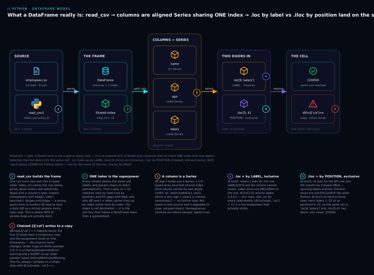
Door 1: plain [] — convenient, ambiguous
Square brackets on a DataFrame are the convenient shorthand, but what they do depends on what you put inside, and that ambiguity is the source of much confusion:
df["name"]              # a STRING  -> one column, as a Series
df[["name", "salary"]]  # a LIST    -> those columns, as a DataFrame
df[df["age"] > 30]      # a MASK    -> the rows where the mask is True
df[1:4]                 # a SLICE   -> ROWS by position (like .iloc!)
Four different behaviours from one operator. A string selects a column; a list of strings selects columns (note the double brackets — the outer [] is selection, the inner [] is the list); a boolean mask selects rows; and a slice selects rows by position. That last one surprises everyone: df[1:4] does not look for columns 1 to 4, it slices rows 1, 2, 3 positionally. And a bare integer is worst of all:
df[6] # KeyError: 6 -- looks for a COLUMN named 6, doesn't find one
Here is the whole [] decision table — memorise which input triggers which behaviour:
| You write | pandas reads it as | Result |
|---|---|---|
df["name"] |
a column name | that column, as a Series |
df[["name", "age"]] |
a list of names | those columns, as a DataFrame |
df[df["age"] > 30] |
a boolean mask | the matching rows |
df[1:4] |
a slice | rows 1–3 by position (end-exclusive) |
df[6] |
a column name 6 |
KeyError: 6 (there is no such column) |
Because [] is overloaded, the guidance is simple: use [] for columns and boolean masks, and use .loc/.iloc for everything involving rows. Those two are explicit and never ambiguous.
Door 2 and 3: .loc (by label) vs .iloc (by position)
.loc and .iloc both take [rows, columns], but they speak different languages. .loc is label-based: you name the row labels and column names you want. .iloc is position-based: you give 0-based integer offsets, ignoring the labels entirely. This is the single most important distinction in pandas selection:
| Aspect | .loc — by label |
.iloc — by position |
|---|---|---|
| Keys mean | Index labels & column names | 0-based integer offsets |
| Single cell | df.loc[6, "salary"] |
df.iloc[5, 4] |
| Whole row | df.loc[6] (label 6) |
df.iloc[5] (6th row) |
| List of rows | df.loc[[1, 6]] |
df.iloc[[0, 5]] |
| Slice | df.loc[2:5] → includes 5 |
df.iloc[1:4] → excludes 4 |
| Slice endpoint | Inclusive (both ends) | Exclusive (Python style) |
| Boolean mask | df.loc[mask] ✓ |
df.iloc[mask.to_numpy()] (needs array) |
| Out-of-range | KeyError |
IndexError |
| Assignment | df.loc[mask, "c"] = x ✓ (the safe way) |
df.iloc[0, 2] = x ✓ |
The inclusive-vs-exclusive slice difference is the one that bites, and our dataset makes it vivid. Because emp_id labels run 1…12 but positions run 0…11, the label is always the position plus one — so the same slice numbers pick different rows:
print(df.loc[2:5, ["name", "age"]]) # LABELS 2..5, inclusive
                 name  age
emp_id
2          Bao Nguyen   29
3        Chidi Okafor   41
4       Diana Ivanova   33
5        Ethan Brooks   26      <- 5 is INCLUDED (4 rows)
print(df.iloc[1:4, [0, 3]]) # POSITIONS 1..4, exclusive
                 name  age
emp_id
2          Bao Nguyen   29
3        Chidi Okafor   41
4       Diana Ivanova   33        <- position 4 (emp_id 5) EXCLUDED (3 rows)
Same 2..5/1..4 numbers, deliberately overlapping rows, different counts: .loc[2:5] returns four rows (labels 2,3,4,5), .iloc[1:4] returns three (positions 1,2,3). Why the asymmetry? .iloc follows Python’s own slicing rule (range(1,4) is 1,2,3 — stop is excluded), while .loc can’t sensibly exclude a label you explicitly named, so it includes both ends. .loc inclusive, .iloc exclusive — tattoo it on your wrist.
Selecting rows and columns together is where .loc/.iloc shine — one clean expression, no chaining:
print(df.loc[[1, 6], ["name", "department", "salary"]])
                name   department  salary
emp_id
1         Ana Garcia  Engineering   98000
6       Fatima Zahra  Engineering  120000
.at and .iat: one scalar, as fast as possible
When you want a single cell — not a row, not a column, one value — .at (label) and .iat (position) are the specialised, faster versions of .loc/.iloc:
print(df.at[6, "salary"])   # => 120000   (label-based scalar)
print(df.iat[5, 4])         # => 120000   (position-based scalar: 6th row, 5th col)
Both reach Fatima Zahra’s salary — one by the row’s label (6), one by its position (5). Reach for .at/.iat inside tight loops or when you truly need just one value; use .loc/.iloc for everything else. The four-way grid:
| Label-based | Position-based | |
|---|---|---|
| Rows / columns / slices | .loc |
.iloc |
| A single scalar (fast) | .at |
.iat |
Boolean filtering: asking questions of your data
The most common thing you do to a DataFrame is filter it — keep the rows matching a condition. You do it by building a boolean mask (a Series of True/False, one per row) and indexing with it. A comparison on a column is a mask:
mask = df["age"] > 30
print(mask.head(4))
emp_id
1     True
2    False
3     True
4     True
Name: age, dtype: bool
Feed that mask to [] (or .loc) and you keep the True rows:
print(df[df["age"] > 30][["name", "age"]])
                 name  age
emp_id
1          Ana Garcia   37
3        Chidi Okafor   41
4       Diana Ivanova   33
6        Fatima Zahra   45
7           Grace Lin   31
9        Ingrid Olsen   39
10        Juan Torres   52
12         Liam Walsh   35
Combining conditions: &, |, ~ — and the parentheses
Real questions have several conditions. Here pandas has two rules that trip up every beginner, and breaking either raises an error:
- Use
&(and),|(or),~(not) — not the Python keywordsand,or,not. - Wrap every condition in parentheses, because
&binds tighter than>.
# Engineers over 30:
m = (df["age"] > 30) & (df["department"] == "Engineering")
print(df[m][["name", "age", "department"]])
                name  age   department
emp_id
1         Ana Garcia   37  Engineering
6       Fatima Zahra   45  Engineering
9       Ingrid Olsen   39  Engineering
Why can’t you write and? Because and asks a single object for its truth value, and a Series of many booleans has no single truth value — so pandas raises:
df[df["age"] > 30 and df["salary"] < 80000]
# ValueError: The truth value of a Series is ambiguous.
#             Use a.empty, a.bool(), a.item(), a.any() or a.all().
And why the parentheses? Because & has higher precedence than >, so df["age"] > 30 & df["department"] == "Engineering" is secretly parsed as df["age"] > (30 & df["department"]) == "Engineering" — pandas tries 30 & <a column> first and blows up:
df["age"] > 30 & df["department"] == "Engineering"
# TypeError: unsupported operand type(s) for &: 'int' and 'StringArray'
The fix for both is the same muscle memory: &/|/~, and parentheses around every comparison.
The readable helpers: .isin, .between, .query
Once conditions pile up, three helpers keep filters readable:
# .isin — membership in a set of values (cleaner than chained ORs)
print(df[df["department"].isin(["Sales", "Support"])][["name", "department"]].head(4))
                 name department
emp_id
3        Chidi Okafor      Sales
4       Diana Ivanova      Sales
5        Ethan Brooks    Support
8          Hassan Ali    Support
# .between — inclusive range on both ends by default
print(df[df["age"].between(30, 40)][["name", "age"]])
                 name  age
emp_id
1          Ana Garcia   37
4       Diana Ivanova   33
7           Grace Lin   31
9        Ingrid Olsen   39
12         Liam Walsh   35
# .query — a string mini-language; no df[...] repetition, and 'and' works here
print(df.query("age > 30 and department == 'Engineering'")[["name", "age"]])
.query reads almost like English and is a joy for interactive work — inside the string you can use and/or, and you reference outside variables with @:
cutoff = 80000
print(df.query("salary >= @cutoff")[["name", "salary"]])
                name  salary
emp_id
1         Ana Garcia   98000
2         Bao Nguyen   88000
6       Fatima Zahra  120000
9       Ingrid Olsen  105000
10       Juan Torres   81000
| Filter tool | Reads as | Note |
|---|---|---|
df[df["c"] > x] |
“rows where c > x” | The everyday mask |
(cond1) & (cond2) |
“both” | &/` |
df["c"].isin([...]) |
“c is one of these” | Replaces long ` |
df["c"].between(lo, hi) |
“lo ≤ c ≤ hi” | Inclusive; inclusive="neither" to change |
~mask |
“not” | Inverts a boolean Series |
df.query("...") |
a readable sentence | and/or ok inside; @var for outside values |
The SettingWithCopyWarning: pandas’ most famous gotcha
You will hit this within your first week, and it is worth truly understanding rather than superstitiously working around. The scenario: you filter, then try to assign to a column of the result.
# Goal: zero out the salary for everyone in Sales.
df[df["department"] == "Sales"]["salary"] = 0
This is chained indexing — two [] operations back to back — and on pandas 3.0 it warns and then silently does nothing:
ChainedAssignmentError: A value is being set on a copy of a DataFrame or Series
through chained assignment. Such chained assignment never works to update the
original DataFrame or Series, because the intermediate object on which we are
setting values always behaves as a copy (due to Copy-on-Write).

Try using '.loc[row_indexer, col_indexer] = value' instead, to perform the
assignment in a single step.
# Check: the Sales salaries are untouched.
print(df[df["department"] == "Sales"]["salary"].tolist())   # => [72000, 76000, 81000]
The salaries did not change. That is the “silent no-op”, and here is exactly why. df[df["department"] == "Sales"] runs first and hands back a new, temporary DataFrame — a copy of the matching rows. Your ["salary"] = 0 then assigns into that temporary, which is discarded on the next line. The original df never saw the write. It is not a pandas bug; it is two separate operations where you thought you had one.
The fix is to make it a single operation with .loc, naming rows and column together so pandas can write in place:
df.loc[df["department"] == "Sales", "salary"] = 0
print(df[df["department"] == "Sales"]["salary"].tolist())   # => [0, 0, 0]
One .loc[mask, "column"] = value — rows and column in one indexer — and the write lands on the real df. This is the pattern for conditional assignment; use it every time.
The version story (you will see both). What the warning is called changed, but the trap and the fix never did. On pandas 1.x and 2.x the same chained assignment raised the legendary
SettingWithCopyWarning:SettingWithCopyWarning: A value is trying to be set on a copy of a slice from a DataFrame. Try using .loc[row_indexer,col_indexer] = value insteadOn pandas 3.0, Copy-on-Write became the default and this is now a
ChainedAssignmentErrorwarning — cleaner, because the old warning was famous for false positives and false negatives. Either way: chained[]for assignment writes to a copy;df.loc[mask, "col"] = valueis the cure. Note that chained indexing for reading (df[df.age > 30]["name"]) is fine — the copy is harmless when you are only looking, not writing.
Since this lesson runs on pandas 3.0 but you will meet 2.x code everywhere, here are the differences that actually change what you see on screen:
| Behaviour | pandas ≤ 2.x | pandas 3.0 |
|---|---|---|
| Text column dtype | object |
str |
Datetime resolution (from parse_dates) |
datetime64[ns] |
datetime64[us] |
| Chained assignment | SettingWithCopyWarning (sometimes worked) |
ChainedAssignmentError + reliable no-op |
| Copy vs view | ambiguous, layout-dependent | Copy-on-Write, on by default |
None of these change the skills in this lesson — .loc, .iloc, masks, and the .loc[mask, col] = value fix are identical on both — only the dtype labels in the output and the warning’s name differ.
Reshaping the frame: columns, index, dtypes, NaN
With selection mastered, the day-to-day edits are quick. Adding a column is assignment to a new name, and it should be a vectorised expression over existing columns — never a loop:
df["salary_k"]   = df["salary"] / 1000          # scale a whole column at once
df["tenure_yrs"] = 2026 - df["hire_date"].dt.year
print(df[["name", "salary", "salary_k", "tenure_yrs"]].head(3))
                name  salary  salary_k  tenure_yrs
emp_id
1         Ana Garcia   98000      98.0           8
2         Bao Nguyen   88000      88.0           5
3       Chidi Okafor   72000      72.0          10
Dropping, renaming, and retyping round out the toolkit:
| Operation | Code | Note |
|---|---|---|
| Add / overwrite column | df["c"] = <Series or scalar> |
Scalar broadcasts to every row |
| Drop columns | df.drop(columns=["a", "b"]) |
Returns a new frame (not in place) |
| Drop rows by label | df.drop(index=[3, 7]) |
By index label |
| Rename columns | df.rename(columns={"old": "new"}) |
Dict of changes |
| Change a dtype | df["age"].astype("float64") |
Fails loudly if a value won’t convert |
| Select by dtype | df.select_dtypes("number") |
e.g. all numeric columns |
print(list(df.select_dtypes("number").columns))
# => ['age', 'salary', 'manager_id', 'salary_k', 'tenure_yrs']
The index: set_index, reset_index, sort_index
The index is not fixed at load time — you promote a column to the index, or push it back to a column, as the task demands. Promoting name to the index lets you look up people by name:
by_name = df.set_index("name")
print(by_name.loc["Fatima Zahra", ["department", "salary"]])
department    Engineering
salary             120000
Name: Fatima Zahra, dtype: object
reset_index() reverses it, turning the index back into an ordinary column (and restoring a default RangeIndex) — you will use it constantly after a groupby in Part 2. And sort_values / sort_index order the rows:
| Method | Does |
|---|---|
df.set_index("col") |
Make a column the row index |
df.reset_index() |
Move the index back to a column |
df.sort_index() |
Sort rows by the index labels |
df.sort_values("col", ascending=False) |
Sort rows by a column’s values |
First look at NaN: the upcasting surprise
Missing data is pandas’ constant companion, and its default marker is NaN — a special float. This produces a surprise every beginner meets: put a missing value into an integer column and the whole column becomes float64. You saw it at load time — manager_id was all whole numbers, yet its dtype is float64 — purely because one row was blank:
print(df["manager_id"].head(3))
emp_id
1    NaN
2    1.0        <- 1.0, not 1 — the column upcast to float
3    1.0
Name: manager_id, dtype: float64
Why? Classic NaN is a floating-point value (it literally comes from the IEEE-754 float standard), and int64 has no way to represent “missing”. So the moment a NaN needs to live in an integer column, pandas upcasts the entire column to float64, where NaN is legal. Your IDs turn into 1.0, 3.0, 5.0. If you need to keep them as integers and allow missing, use pandas’ nullable Int64 (capital I):
print(df["manager_id"].astype("Int64").head(3))
emp_id
1    <NA>       <- a proper missing marker, and...
2       1       <- ...the values stay integers
3       1
Name: manager_id, dtype: Int64
Missing data gets its own full section in Part 2 (isna, fillna, dropna, and how NaN behaves in every operation). For now, just recognise the tell: an integer-looking column showing up as float64 almost always means it has a missing value.
Dropping to NumPy: .values and .to_numpy()
Under every DataFrame are NumPy arrays, and sometimes you need the raw array — to hand to scikit-learn, or to run a NumPy operation pandas doesn’t wrap. .to_numpy() is the modern way (.values is the older attribute; prefer .to_numpy()):
arr = df[["age", "salary"]].to_numpy()
print(type(arr).__name__, arr.dtype, arr.shape)   # => ndarray int64 (12, 2)
You get a plain 2-D NumPy array — labels stripped, one shared dtype — which is exactly what numerical libraries expect. This is the seam between pandas (labelled, heterogeneous, for wrangling) and NumPy (raw, homogeneous, for math).
Why vectorised, not loops: measure it
The cardinal rule of pandas is never loop over rows. Column operations are vectorised — they run in C over the whole NumPy array at once. To feel the difference, add two million-row columns two ways: element-by-element with apply(axis=1), and vectorised:
import numpy as np, timeit
big = pd.DataFrame({"a": np.random.rand(1_000_000),
                    "b": np.random.rand(1_000_000)})

t_apply = timeit.timeit(lambda: big.apply(lambda r: r["a"] + r["b"], axis=1), number=1)
t_vec   = timeit.timeit(lambda: big["a"] + big["b"], number=1)
print(f"apply(axis=1): {t_apply:.3f} s")   # => apply(axis=1): 2.475 s
print(f"vectorised   : {t_vec:.5f} s")     # => vectorised   : 0.00195 s
print(f"speedup      : {t_apply / t_vec:.0f}x")   # => speedup: ~1266x
On this machine the vectorised version is over a thousand times faster (your exact numbers will vary, but the order of magnitude won’t). apply(axis=1) calls your Python function once per row — a million times — while big["a"] + big["b"] is a single NumPy add. The lesson: express what you want as whole-column arithmetic, and only fall back to apply when there is genuinely no vectorised way.
| Approach | Speed on 1M rows | When |
|---|---|---|
df["a"] + df["b"] (vectorised) |
~2 ms | Default — always try this first |
df["c"].map(func) |
moderate | Element-wise on one column, no vector form |
df.apply(func, axis=1) |
~2.5 s | Last resort — needs the whole row at once |
for _, row in df.iterrows() |
slowest | Almost never; a code smell |
Hands-on lab
Run this end to end. It needs pandas in a virtual environment — nothing else. Each step shows the command, what you should see, and the one-line “what just happened”.
Step 0 — Set up an isolated environment.
python3 -m venv .venv
source .venv/bin/activate          # Windows: .venv\Scripts\activate
pip install pandas
python -c "import pandas as pd; print(pd.__version__)"   # 3.0.x (or 2.x — notes below)
What just happened: a clean venv with pandas. If you are on pandas 2.x, everything works — you will see object instead of str for text columns and the classic SettingWithCopyWarning in Step 6.
Step 1 — Create the dataset and load it properly. Put the CSV-building snippet from the “Loading real data” section into make_data.py, run it once (python make_data.py), then in a Python shell:
import pandas as pd
df = pd.read_csv("employees.csv", index_col="emp_id", parse_dates=["hire_date"])
What just happened: emp_id is the row index and hire_date is a real datetime — the two things a naïve load gets wrong.
Step 2 — Inspect before you trust.
df.shape          # (12, 8)
df.info()         # types + non-null counts; note manager_id is 11 non-null
df.describe()     # median salary 74000, ages 24..52
df.dtypes         # hire_date is datetime64[us]; text is str (or object on 2.x)
What just happened: you confirmed the load. info() flagged the one missing manager_id; describe() gave the numeric shape.
Step 3 — Select columns and rows three ways.
df["name"]                              # [] -> one column (Series)
df[["name", "salary"]].head(3)          # [] with a list -> columns (DataFrame)
df.loc[2:5, ["name", "age"]]            # .loc -> LABELS 2..5 inclusive (4 rows)
df.iloc[1:4, [0, 3]]                    # .iloc -> POSITIONS 1..3 exclusive (3 rows)
df.at[6, "salary"]                      # 120000 — one scalar by label
What just happened: you saw all three doors. Note .loc[2:5] returned four rows and .iloc[1:4] three — inclusive vs exclusive, live.
Step 4 — Filter with combined masks and .query.
df[(df["age"] > 30) & (df["department"] == "Engineering")][["name", "age"]]
df[df["department"].isin(["Sales", "Support"])][["name", "department"]]
df.query("age > 30 and salary > 90000")[["name", "age", "salary"]]
What just happened: three ways to ask a two-part question. The & version needs parentheses; .query lets you write and.
Step 5 — Reproduce the silent no-op, then fix it.
df[df["department"] == "Sales"]["salary"] = 0        # WARNS, then does nothing
df[df["department"] == "Sales"]["salary"].tolist()   # still [72000, 76000, 81000]

df.loc[df["department"] == "Sales", "salary"] = 0     # the fix
df[df["department"] == "Sales"]["salary"].tolist()    # now [0, 0, 0]
What just happened: chained [] wrote to a copy (no change); the single .loc[mask, col] = value wrote to the real frame. This is the muscle memory to keep.
Step 6 — Set/reset the index, add a computed column.
by_name = df.set_index("name")
by_name.loc["Fatima Zahra", "salary"]        # 120000 — lookup by name
by_name.reset_index().columns                # 'name' is a column again
df["tenure_yrs"] = 2026 - df["hire_date"].dt.year   # vectorised, no loop
df[["name", "tenure_yrs"]].head(3)
What just happened: you moved a column in and out of the index, and added a new column as one whole-column expression. You have now touched every core operation in the lesson.
⚠️
df.drop(...),df.rename(...), anddf.sort_values(...)return a new DataFrame by default — they do not changedfin place. Assign the result (df = df.drop(...)) or you will wonder why “nothing happened”.
Common mistakes and troubleshooting
| Symptom / traceback | Cause | Fix |
|---|---|---|
ChainedAssignmentError (3.0) / SettingWithCopyWarning (≤2.x), and the value doesn’t change |
Chained indexing df[mask]["col"] = x assigns to a temporary copy |
Single step: df.loc[mask, "col"] = x |
.loc[2:5] returns one more row than expected |
.loc slices are inclusive of the end label |
Use .iloc for exclusive/positional slices, or subtract one |
KeyError: 'salery' |
Misspelled column, or the column isn’t there | print(df.columns); fix the name |
KeyError: 999 from df.loc[999] |
No row has that label | Check df.index; use .iloc for a position, or .reindex/.get |
ValueError: The truth value of a Series is ambiguous |
Used and/or between two masks |
Use &/` |
TypeError: unsupported operand type(s) for &: 'int' and ... |
Missing parentheses; & binds tighter than > |
(df.a > 1) & (df.b < 2) |
Integer column shows up as float64 |
A missing value forced NaN, which is a float → upcast |
Expected; use Int64 (nullable) to keep integers |
df["new"] = other_series gives unexpected NaNs |
Assignment aligns on the index; labels didn’t match | Match the index, or assign other_series.to_numpy() to ignore labels |
Text column is object, .str/date methods slow or odd |
Mixed types, or older pandas’ default string storage | astype("str"); force dtype= at load; clean mixed values |
df.drop(...) “did nothing” |
It returns a new frame; not in place by default | df = df.drop(...) (or pass inplace=True, discouraged) |
| Dates won’t sort or subtract | hire_date loaded as text, not datetime |
parse_dates=["hire_date"] at load, or pd.to_datetime(...) |
SettingWithCopyWarning after a filter you did mean to edit |
You edited a slice that may be a view or a copy | Take an explicit .copy() first, then edit the copy |
Three gotchas deserve extra words, because they cost the most hours.
1. [] is overloaded — prefer .loc/.iloc for rows. Because df["x"] means “column x” but df[1:4] means “rows 1–3” and df[mask] means “these rows”, the plain bracket is a small guessing game. The habit that removes the ambiguity forever: use [] only to grab columns or apply a boolean mask, and use .loc/.iloc any time a row is involved. Explicit beats clever.
2. Assignment aligns on the index — this is a feature that looks like a bug. When you write df["bonus"] = some_series, pandas does not paste values in row order; it matches some_series’ labels against df’s index. Watch:
bonus = pd.Series([1000, 2000, 3000], index=[3, 99, 7])   # label 99 isn't in df
df["bonus"] = bonus
print(df[["name", "bonus"]].loc[[2, 3, 7]])
                name   bonus
emp_id
2         Bao Nguyen     NaN     <- no label 2 in bonus -> NaN
3       Chidi Okafor  1000.0     <- label 3 matched
7          Grace Lin  3000.0     <- label 7 matched
Employee 3 got 1000 and 7 got 3000 because their labels matched; employee 2 got NaN (absent from bonus); and the 99 in bonus — a label not in df — was silently dropped. If you truly want positional assignment, strip the labels with .to_numpy(): df["bonus"] = bonus.to_numpy() (lengths must match). Ninety percent of “why is my new column full of NaN?” is this alignment doing exactly what it promised.
3. The silent no-op is silent for a reason. The reason chained assignment can’t work is worth internalising: df[mask] is a function call that returns a new object. Assigning to that object’s column mutates the return value, which has no connection back to df. Under Copy-on-Write (pandas 3.0), pandas can prove the write is pointless and warns you; under older pandas it sometimes worked and sometimes didn’t depending on memory layout, which is exactly why SettingWithCopyWarning was so hated. df.loc[mask, "col"] = value sidesteps the whole mess by being one indexing operation that pandas can resolve to a real, in-place write.
Cheat-sheet
Bookmark this. It answers “how do I select / filter / edit this DataFrame?” without a web search.
| Task | Code |
|---|---|
| Load a CSV well | pd.read_csv("f.csv", index_col="id", parse_dates=["d"]) |
| First / last rows | df.head() · df.tail() |
| Shape, types, health | df.shape · df.dtypes · df.info() |
| Summary stats | df.describe() · df.describe(include="all") |
| One column (Series) | df["col"] or df.col |
| Several columns | df[["a", "b"]] |
| Rows by label | df.loc[label] · df.loc[l1:l2] (inclusive) |
| Rows by position | df.iloc[pos] · df.iloc[a:b] (exclusive) |
| Rows and columns | df.loc[rows, cols] · df.iloc[rows, cols] |
| One scalar, fast | df.at[label, "col"] · df.iat[i, j] |
| Filter (mask) | df[df["age"] > 30] |
| Combine conditions | df[(a) & (b)] · `df[(a) |
| Membership / range | df[df["c"].isin([...])] · df[df["c"].between(lo, hi)] |
| Readable filter | df.query("age > 30 and dept == 'Eng'") |
| Conditional write | df.loc[mask, "col"] = value ← the safe pattern |
| Add column | df["new"] = df["a"] * df["b"] |
| Drop / rename | df.drop(columns=[...]) · df.rename(columns={...}) |
| Change type | df["c"] = df["c"].astype("float64") (or "Int64") |
| Move column ↔ index | df.set_index("c") · df.reset_index() |
| Sort | df.sort_values("c") · df.sort_index() |
| To NumPy | df.to_numpy() · df["c"].to_numpy() |
| Value distribution | df["c"].value_counts() |
Interview and exam questions
Q: What is a Series, and how does it differ from a NumPy array and a Python dict?
A: A Series is a one-dimensional labelled array — a typed values array (NumPy-backed) plus an index of labels. Unlike a NumPy array it has an index and aligns by label; unlike a dict its values are one dtype and it supports vectorised math (s * 2, s > 30). It sits between the two, giving you dict-style lookup with array-style speed.
Q: A DataFrame is best described as what, in one phrase? A: An ordered dict of Series that all share one row index. Each column is a Series with its own dtype; all columns are aligned on the same index. That shared index is what makes joins, alignment, and label-based selection work.
Q: Explain the difference between .loc and .iloc, including the slice endpoint behaviour.
A: .loc is label-based — you pass index labels and column names — and its slices are inclusive of the end label (df.loc[2:5] includes 5). .iloc is position-based — 0-based integer offsets, ignoring labels — and its slices are exclusive like normal Python (df.iloc[1:4] stops before 4). Use .loc when you know the labels, .iloc when you know the positions.
Q: What does df[df["age"] > 30] return, and what is the object inside the brackets?
A: It returns the rows where the condition is True. The inner df["age"] > 30 is a boolean Series (a mask) — one True/False per row, aligned to the index — and indexing a DataFrame with a boolean mask keeps the True rows.
Q: Why does df[df.a > 1 and df.b < 2] fail, and how do you fix it?
A: and needs a single truth value, but a boolean Series has many, so it raises ValueError: The truth value of a Series is ambiguous. Use the element-wise &, and parenthesise each comparison because & binds tighter than >: df[(df.a > 1) & (df.b < 2)].
Q: What is the SettingWithCopyWarning / ChainedAssignmentError, and what’s the correct pattern?
A: It fires on chained indexing like df[mask]["col"] = x. The first [] returns a temporary copy, so the assignment lands on the copy and the original is unchanged (a silent no-op). Fix it with a single indexer: df.loc[mask, "col"] = x. On pandas 3.0 (Copy-on-Write) it’s a ChainedAssignmentError warning; on 2.x and earlier it’s SettingWithCopyWarning — same cause, same fix.
Q: You load a CSV and an integer ID column comes in as float64. Why, and what are your options?
A: The column has at least one missing value. Classic NaN is a float and int64 can’t hold it, so pandas upcasts the whole column to float64. Options: accept the float, or convert to the nullable Int64 dtype (astype("Int64")) which keeps integers and uses <NA> for missing, or fill/clean the missing values first.
Q (practical): Give everyone in the Sales department a 10% raise, in one line.
A: df.loc[df["department"] == "Sales", "salary"] *= 1.1 — a boolean mask picks the rows, the column name picks the target, and the single .loc write is in place, so it actually sticks (unlike chained indexing).
Q: You assign df["x"] = a_series and get a column full of NaN. What happened?
A: Assignment aligns on the index. a_series’ labels didn’t match df’s index, so unmatched rows became NaN and any extra labels in a_series were dropped. Either give a_series a matching index, or assign a_series.to_numpy() to force positional (order-based) assignment.
Q: When would you drop from pandas to df.to_numpy()?
A: When a downstream library wants a raw array (scikit-learn’s fit, a NumPy-only routine), or for a numeric operation pandas doesn’t wrap. You lose the labels and get one shared dtype — fine for math, which is exactly the boundary between pandas (labelled wrangling) and NumPy (raw computation).
Q (practical): How do you select the name and salary of the 6th through 10th rows regardless of their index labels?
A: By position with .iloc: df.iloc[5:10][["name", "salary"]] (positions 5–9, since .iloc is 0-based and end-exclusive). Using .loc[6:10] would be wrong here — that’s label-based and inclusive.
Q: Why is df.apply(func, axis=1) slow, and what should you reach for first?
A: apply(axis=1) calls a Python function once per row, so on a million rows it’s a million Python calls — often ~1000× slower than the vectorised form. Reach first for whole-column arithmetic (df["a"] + df["b"]), which runs once in C over the underlying NumPy arrays.
Key takeaways
- A Series is a 1-D array plus an index; a DataFrame is an ordered dict of Series sharing one index. The index is the thing that makes pandas more than a spreadsheet — it drives alignment, selection, and assignment.
- Automatic label alignment is the superpower. Combining Series or assigning a Series matches on labels, not position, filling gaps with
NaN. Most surpriseNaNs are alignment working as designed. - Load deliberately, inspect immediately. Use
read_csvwithindex_col,parse_dates, anddtype; then runhead,info,describe,dtypes,shapebefore trusting anything. Most pandas bugs are really load-time type bugs. .locis label-based and inclusive;.ilocis position-based and exclusive. Use[]only for columns and boolean masks; use.loc/.ilocwhenever a row is involved; use.at/.iatfor a single scalar.- Filter with
&,|,~and parentheses — neverand/or. Reach for.isin,.between, and.queryto keep multi-condition filters readable. - Chained assignment
df[mask]["col"] = xwrites to a copy and silently fails. Always usedf.loc[mask, "col"] = value. The warning’s name changed across versions (SettingWithCopyWarning→ChainedAssignmentError); the fix never did. NaNis a float, so a missing value upcasts an int column tofloat64. Use nullableInt64to keep integers with missing data — full missing-data treatment comes in Part 2.- Never loop over rows. Express operations as whole-column arithmetic (vectorised NumPy underneath); it is often a thousand times faster than
apply(axis=1). Part 2 builds on all of this withgroupby,merge, and reshaping.