Part 1 gave you the two containers — the Series and the DataFrame — and taught you to select, filter and index them. That is how you look at data. This lesson is how you answer questions with it, and almost every real question is one of three shapes: summarise by group (“revenue per region”), join two tables (“attach each order to its customer”), and cope with the holes (“half the rows are missing a price”). Those three — GroupBy, merge, and missing data — are the daily work of data wrangling, and each one has a small, sharp set of traps that quietly return the wrong number instead of raising an error.
Here is the shape of the problem, in the code most analyses actually start from:
total = 0
for row in orders:                       # a Python loop over rows
    if row["region"] == "North":
        total += row["units"] * row["price"]
It works, for one region, until the boss asks for all regions, then a per-region average, then “but only regions with at least three orders,” then “joined to the customer table,” and your loop grows a second loop, a dictionary of running totals, and a bug where a missing price crashes on row 400. Pandas replaces that entire genre of code with three method calls — groupby, merge, and fillna — that are faster, shorter, and correct about the edge cases you would have gotten wrong by hand. The catch is that “correct” depends on you picking the right one, and this lesson is about that choice.
Every snippet here is executed on Python 3.12 with pandas 3.0.3 and NumPy 2.5. Pandas 3.0 changed several defaults that bite (Copy-on-Write is always on, string columns report a
strdtype, datetimes default to microsecond resolution, and chained assignment now raises rather than warns) — where a behaviour differs from the pandas 2.x you may have installed, there is a version note.
Why this matters
Aggregation-by-group is the single most common operation in data work, and it is exactly the operation a beginner writes worst by hand. A for loop with a dictionary of running totals is slow, it is verbose, and it silently mishandles missing values — a None price becomes a TypeError halfway through, or worse, gets counted as zero. Pandas’ groupby does the same job in one line, in C, and with a defined answer for the empty group and the null value. But it hands you four ways to apply your function to each group — agg, transform, filter, apply — and choosing wrong is the difference between a 3-row summary and a 10-row annotated frame. Most “why is my result the wrong shape?” confusion traces back to reaching for apply when you wanted transform.
Merging is the second pillar, and it is where rows silently appear and disappear. A join is a promise about how two tables line up on a key, and pandas will keep whatever promise you actually made — not the one you meant. Ask for the default how='inner' and every unmatched row vanishes with no warning; feed it a key that is duplicated on both sides and it hands you a many-to-many cross product that quietly multiplies your row count and double-counts your revenue. The fix is not vigilance, it is validate= — you state the cardinality you expect and let pandas raise the moment the data breaks it.
Missing data is the third, and it is the one people most want to wish away. Real data has holes: a survey question skipped, a sensor offline, a customer who never gave a phone number, a key that matched nothing in the join. Pandas represents those holes with a small zoo of sentinels — NaN, None, NaT, and the modern pd.NA — and the first surprise is structural: put one missing value in an integer column and the whole column becomes float64, because the classic NaN is a float and an integer column has no room for it. Detecting, counting and filling those holes is routine; doing it honestly — knowing when a fillna(0) is a lie that corrupts your mean — is the mark of someone who has been burned.
Hold one sentence for the whole lesson: pandas will almost never raise on a wrong-but-plausible operation; it will hand you a wrong number. A dropped row, a doubled row, a NaN-poisoned average — none of them throw. Your defence is knowing which method has which shape, stating your join’s cardinality, and looking at your row count before and after. This lesson builds all three habits on real, executed output.
GroupBy: split → apply → combine
Every groupby is the same three-step pattern, and naming the steps out loud is most of the battle. Split the rows into groups by a key. Apply a function to each group independently. Combine the results back into one object. That pattern — split-apply-combine — is the mental model behind groupby, pivot_table, crosstab, and even the way you should think about a merge.
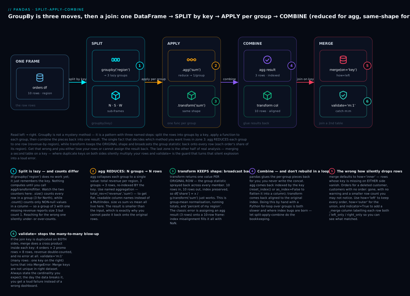
Read the diagram left to right. The one fact that decides which method you want lives in the APPLY and COMBINE zones: agg reduces each group to a single row, while transform keeps the original shape and sprays the group statistic back onto every row. The badges mark the traps — the lazy split that does nothing until you call a method (1), the reduce-vs-broadcast fork (2, 3), the index-misalignment that fills a mis-shaped assignment with NaN (4), the wrong how that drops rows (5), and the validate= guard that stops a silent many-to-many blow-up (6).
Start with a small sales frame and the simplest possible aggregation:
import pandas as pd
import numpy as np

sales = pd.DataFrame({
    "region": ["North", "North", "South", "South", "West", "West", "North"],
    "rep":    ["Asha", "Bala", "Chen", "Diya", "Esha", "Faiz", "Asha"],
    "units":  [10, 5, 8, 12, 7, 3, 6],
    "revenue":[2000.0, 900.0, 1600.0, 2400.0, 1400.0, np.nan, 1200.0],
})

print(sales.groupby("region")["revenue"].mean())
region
North    1366.666667
South    2000.000000
West     1400.000000
Name: revenue, dtype: float64
That one line is split-apply-combine: split by region, apply mean to each group’s revenue, combine into a Series indexed by region. Notice the mean of West is 1400.0, not 700.0 — the NaN in West’s revenue was skipped, not treated as zero. That skipna=True default is a kindness most of the time and a trap when you forget it.
The object sales.groupby("region") returns is lazy. It does no computation and holds no result; it only remembers the key. Nothing happens until you call an aggregation on it — which is why you can build it once and call .mean(), .sum() and .size() on it cheaply.
size vs count — and why the difference is NaN
The two most-confused reductions are size and count, and the entire distinction is null handling:
g = sales.groupby("region")
print(g.size())            # rows per group — counts everything
print(g["revenue"].count())   # non-null values in the column
region
North    3
South    2
West     2
dtype: int64
region
North    3
South    2
West     1
Name: revenue, dtype: int64
West has two rows (size = 2) but only one non-null revenue (count = 1), because Faiz’s revenue is NaN. size counts rows; count counts values that are actually there. Reach for size when you want “how many records,” and count when you want “how many usable numbers” — mixing them up is a silent under- or over-count that never raises.
| Reduction | Counts | Ignores NaN? |
Returns |
|---|---|---|---|
g.size() |
every row in the group | no — counts NaN rows |
Series, one per group (no column needed) |
g.count() |
non-null values, per column | yes | DataFrame (or Series for one column) |
g["c"].nunique() |
distinct non-null values | yes (drop NaN by default) |
Series |
len(g) |
number of groups | n/a | a plain int |
agg — one function or many
agg (alias aggregate) is the reduce step. Give it one function, a list of functions, or a per-column dictionary:
# many functions on one column
print(sales.groupby("region")["revenue"].agg(["sum", "mean", "count", "max"]))
           sum         mean  count     max
region
North   4100.0  1366.666667      3  2000.0
South   4000.0  2000.000000      2  2400.0
West    1400.0  1400.000000      1  1400.0
# a different function per column
print(sales.groupby("region").agg({"units": "sum", "revenue": "mean"}))
        units      revenue
region
North      21  1366.666667
South      20  2000.000000
West       10  1400.000000
The list form is convenient but leaves you with clumsy column names (sum, mean) and, when you aggregate several columns several ways, an awkward two-level MultiIndex on the columns. The cure is named aggregation — the clearest way to write an agg, and the one to reach for by default:
print(sales.groupby("region").agg(
    total_rev=("revenue", "sum"),
    avg_units=("units", "mean"),
    n=("rep", "size"),
))
        total_rev  avg_units  n
region
North      4100.0        7.0  3
South      4000.0       10.0  2
West       1400.0        5.0  2
Each keyword becomes a flat, named output column, and its value is a (column, function) tuple that says exactly what to aggregate and how. It reads like a spec, the column names are yours, and there is no MultiIndex to flatten afterwards. The fully spelled-out form uses pd.NamedAgg(column=..., aggfunc=...), which is identical to the tuple but self-documenting:
print(sales.groupby("region").agg(
    total_rev=pd.NamedAgg(column="revenue", aggfunc="sum"),
))
Grouping by multiple keys produces a MultiIndex, one level per key:
print(sales.groupby(["region", "rep"])["units"].sum())
region  rep
North   Asha    16
        Bala     5
South   Chen     8
        Diya    12
West    Esha     7
        Faiz     3
Name: units, dtype: int64
Asha appears once per region-rep combination with her two North orders summed to 16. If you would rather have flat columns than a grouped index — for a subsequent merge, or a CSV export — pass as_index=False, or call .reset_index() on the result. They reach the same place:
print(sales.groupby("region", as_index=False)["units"].sum())
  region  units
0  North     21
1  South     20
2   West     10
Common agg functions (string names) |
Meaning |
|---|---|
"sum", "mean", "median", "min", "max" |
the obvious reductions; all skip NaN |
"count", "size" |
non-null count vs total rows (see above) |
"std", "var", "sem" |
spread; NaN-skipping |
"first", "last", "nth" |
positional pick within each group |
"nunique" |
distinct non-null values |
"idxmax", "idxmin" |
the index label of the max/min, not the value |
a callable, e.g. lambda s: s.max() - s.min() |
any function taking a Series → scalar |
The three shapes: agg, transform, filter (and apply)
This is the section that fixes most GroupBy confusion. agg, transform and filter all “apply a function to each group,” but they differ in the shape of what comes back, and that shape is the whole reason you would choose one over another.
| Method | What the function receives | What it returns | Output shape | Use it for |
|---|---|---|---|---|
agg |
one column (a Series) per group |
one scalar per group | reduced — N groups → N rows | summaries: total/mean/max per group |
transform |
one column (a Series) per group |
a Series the same length as the group |
same shape as the input — broadcast back | group-relative values: normalise, share, running fill |
filter |
the whole group (a DataFrame) |
a single True/False |
subset — whole groups kept or dropped | keep/drop groups by a group property |
apply |
the whole group (a DataFrame) |
anything | whatever you return | the flexible, slow fallback for the rest |
Work an example of each on the same sales frame.
agg reduces. You have seen it: sales.groupby("region")["revenue"].sum() turns three groups into three numbers. The result is smaller than the input, indexed by the key. This is exactly why you cannot paste it back onto the original rows — the shapes do not match.
transform keeps the shape. It returns one value per original row — the group statistic broadcast back across every member of the group:
sales2 = sales.copy()
sales2["region_avg_units"] = sales2.groupby("region")["units"].transform("mean")
sales2["share_of_region"] = (
    sales2["units"] / sales2.groupby("region")["units"].transform("sum")
)
print(sales2[["region", "rep", "units", "region_avg_units", "share_of_region"]])
  region   rep  units  region_avg_units  share_of_region
0  North  Asha     10               7.0         0.476190
1  North  Bala      5               7.0         0.238095
2  South  Chen      8              10.0         0.400000
3  South  Diya     12              10.0         0.600000
4   West  Esha      7               5.0         0.700000
5   West  Faiz      3               5.0         0.300000
6  North  Asha      6               7.0         0.285714
Seven rows in, seven rows out. Every North row carries North’s average (7.0); every row’s share_of_region is its units over its region’s total. Because the result is aligned to the original index, sales2["share"] = ... just works — no merge, no reset. This is group-mean normalisation, “percent of my category,” running group fills, z-scores within a group. Any time you want to compare a row to its group and keep the row, you want transform.
filter keeps or drops whole groups. The function receives the entire group as a DataFrame and returns one boolean; the group survives only if it returns True:
# keep only regions with at least 3 orders
print(sales.groupby("region").filter(lambda d: len(d) >= 3))
  region   rep  units  revenue
0  North  Asha     10   2000.0
1  North  Bala      5    900.0
6  North  Asha      6   1200.0
Only North has three or more rows, so South and West are dropped entirely — every one of their rows is gone, and the ones that remain keep their original index labels (0, 1, 6). This is “drop small groups,” “keep customers with more than five purchases,” “ignore any day with fewer than N readings.”
apply is the flexible, slow fallback. When your per-group logic returns something none of the three above can express — a different-shaped frame, a scalar computed from several columns, a whole reshaped sub-table — reach for apply. It receives the whole group and lets you return anything:
def top_rep(group):
    return group.loc[group["units"].idxmax(), "rep"]   # the rep with the most units

print(sales.groupby("region").apply(top_rep, include_groups=False))
region
North    Asha
South    Diya
West     Esha
dtype: str
That dtype: str is a pandas 3.0 detail — string results now report the dedicated str dtype rather than the old object; on pandas 2.x you would see dtype: object. apply is the Swiss-army knife, and like most Swiss-army knives it is the wrong tool whenever a dedicated one exists: it runs your Python function once per group with per-group overhead, so it is materially slower than agg/transform, which push the loop into C. Use it only when the shape you need genuinely does not fit the other three.
Version note (pandas 3.0):
applyon a GroupBy now excludes the grouping columns from the frame your function receives. Touchinggroup["region"]inside the function raisesKeyError: 'region'. In pandas 2.2 this emitted aDeprecationWarningand you silenced it withinclude_groups=False; in pandas 3.0 exclusion is the only behaviour, and passinginclude_groups=TrueraisesValueError: include_groups=True is no longer allowed.If you need the key inside the function, use the group name (for name, grp in gb:) orreset_index()first.
The shape trap, made concrete
The classic mistake is assigning an agg result back onto the original frame, expecting transform’s behaviour:
sales["bad"] = sales.groupby("region")["units"].sum()   # sum() has 3 rows; sales has 7
print(sales[["region", "units", "bad"]])
  region  units  bad
0  North     10  NaN
1  North      5  NaN
2  South      8  NaN
3  South     12  NaN
4   West      7  NaN
5   West      3  NaN
6  North      6  NaN
Every value is NaN, and nothing raised. The right-hand side is a Series indexed by region (North, South, West); the left-hand side is a column on a frame indexed by 0..6. Pandas aligns them on the index, finds no overlap between region names and integers, and fills the lot with NaN. The fix is transform("sum"), which returns a result already aligned to the original index. When a group calculation “comes out all NaN,” this index-misalignment is the first thing to check.
pivot_table and crosstab
A pivot_table is groupby wearing a spreadsheet’s clothes: it groups by one field down the rows and another across the columns, and fills the cells with an aggregate. Anything a pivot table does, a groupby on two keys plus an unstack also does — but the pivot form reads better when you want a matrix.
sales3 = sales.assign(quarter=["Q1","Q1","Q1","Q2","Q2","Q2","Q2"])
print(pd.pivot_table(sales3, index="region", columns="quarter",
                     values="units", aggfunc="sum", fill_value=0))
quarter  Q1  Q2
region
North    15   6
South     8  12
West      0  10
index is the row key, columns is the column key, values is what gets aggregated, aggfunc is how, and fill_value replaces the NaN in empty cells — West made no Q1 sales, so its cell would be NaN but shows 0. Add margins=True for row and column totals:
pt = pd.pivot_table(sales, index="region", values=["units", "revenue"],
                    aggfunc="sum", margins=True, margins_name="Total")
print(pt)
        revenue  units
region
North    4100.0     21
South    4000.0     20
West     1400.0     10
Total    9500.0     48
pivot_table parameter |
Does |
|---|---|
index |
field(s) that become the row labels (the group-by-down key) |
columns |
field(s) that become the column labels (the group-by-across key) |
values |
the column(s) to aggregate into the cells |
aggfunc |
"sum", "mean", a list, or a per-value dict; default is "mean" |
fill_value |
replaces NaN in empty cells |
margins / margins_name |
add a grand-total row and column, named "All" by default |
observed |
for categorical keys, whether to show unobserved combinations (default True in 3.0) |
dropna |
drop columns whose entries are all NaN (default True) |
pivot_table aggregates (it expects many rows per cell and reduces them). Its cousin pivot merely reshapes and raises ValueError on duplicate index/column pairs — reach for pivot_table whenever a cell could hold more than one value. And crosstab is a pivot_table specialised for frequency counts: pass it two (or more) Series and it tabulates how often each combination occurs.
print(pd.crosstab(sales3["region"], sales3["quarter"]))
quarter  Q1  Q2
region
North     2   1
South     1   1
West      0   2
crosstab counts by default (North had 2 orders in Q1). Its most useful trick is normalize, turning counts into proportions — normalize="index" makes each row sum to 1:
print(pd.crosstab(sales3["region"], sales3["quarter"], normalize="index").round(2))
quarter    Q1    Q2
region
North    0.67  0.33
South    0.50  0.50
West     0.00  1.00
| Tool | Best for | Aggregates? |
|---|---|---|
groupby(...).agg(...) |
any reduction, especially to a long/tidy result | yes |
pivot_table |
a rectangular matrix of an aggregate, with margins | yes |
pivot |
pure reshape, one value per cell guaranteed | no — raises on duplicates |
crosstab |
frequency/contingency tables, with normalize |
counts (or an aggregate via values/aggfunc) |
Merging and joining DataFrames
Real data lives in more than one table. Orders reference a customer by cust_id; the customer’s name and city live in a separate customers table. Bringing them together on the shared key is a join (SQL’s word) or a merge (pandas’ word). Get the join right and analysis is easy; get it subtly wrong and rows appear or vanish without a sound.
customers = pd.DataFrame({
    "cust_id": [1, 2, 3, 4],
    "name": ["Asha", "Bala", "Chen", "Diya"],
    "city": ["Pune", "Delhi", "Pune", "Surat"],
})
orders = pd.DataFrame({
    "order_id": [101, 102, 103, 104, 105],
    "cust_id":  [1, 1, 2, 3, 99],    # cust 99 has no customer row; cust 4 has no order
    "amount":   [250.0, 400.0, 120.0, 900.0, 50.0],
})
The single most consequential argument is how, which decides which rows survive when a key matches on one side but not the other. The default is inner, and the default is where rows silently disappear.
how |
Keeps | In this example |
|---|---|---|
"inner" (default) |
only keys present in both | 4 rows — order 105 (cust 99) dropped, customer 4 (no order) dropped |
"left" |
all left rows; NaN for unmatched right |
5 rows — order 105 kept with NaN name |
"right" |
all right rows; NaN for unmatched left |
5 rows — customer 4 kept with NaN order |
"outer" |
the union of keys from both sides | 6 rows — both the orphan order and the order-less customer |
"cross" |
every left row × every right row | 20 rows — a deliberate cross product, no key |
print(pd.merge(orders, customers, on="cust_id", how="left"))
   order_id  cust_id  amount  name   city
0       101        1   250.0  Asha   Pune
1       102        1   400.0  Asha   Pune
2       103        2   120.0  Bala  Delhi
3       104        3   900.0  Chen   Pune
4       105       99    50.0   NaN    NaN
how="left" keeps all five orders; order 105 has no matching customer, so name and city are NaN. Had you used the default inner, that row — a real ₹50 order — would have silently dropped, and your revenue total would be ₹50 short with nothing to indicate why. Check your row count before and after a merge. When you genuinely want to know what matched, indicator=True adds a _merge column labelling every row:
print(pd.merge(orders, customers, on="cust_id", how="outer", indicator=True))
   order_id  cust_id  amount  name   city      _merge
0     101.0        1   250.0  Asha   Pune        both
1     102.0        1   400.0  Asha   Pune        both
2     103.0        2   120.0  Bala  Delhi        both
3     104.0        3   900.0  Chen   Pune        both
4       NaN        4     NaN  Diya  Surat  right_only
5     105.0       99    50.0   NaN    NaN   left_only
Two things to notice. _merge cleanly separates the orphan order (left_only) from the customer with no orders (right_only) — invaluable for a reconciliation. And order_id has turned into 101.0, a float: the outer join introduced a NaN (customer 4’s missing order), and an integer column cannot hold NaN, so the whole column upcast to float64. That upcast is the theme of the next section, arriving here uninvited.
When the key has different names on each side, use left_on/right_on; when the join is on the index, use left_index/right_index or the .join method. When non-key columns collide, suffixes disambiguates them:
a = pd.DataFrame({"cust_id":[1,2], "score":[10,20]})
b = pd.DataFrame({"cust_id":[1,2], "score":[99,88]})
print(pd.merge(a, b, on="cust_id", suffixes=("_2023", "_2024")))
   cust_id  score_2023  score_2024
0        1          10          99
1        2          20          88
Without suffixes, colliding columns get the defaults _x and _y — a smell in production code, because score_x tells the next reader nothing. Name them.
merge parameter |
Does |
|---|---|
on |
column name(s) present in both frames to join on |
left_on / right_on |
join keys with different names on each side |
left_index / right_index |
join on the index instead of a column |
how |
inner / left / right / outer / cross — which rows survive |
suffixes |
rename colliding non-key columns (default ("_x", "_y")) |
indicator |
add a _merge column: both / left_only / right_only |
validate |
assert cardinality: "1:1", "1:m", "m:1", "m:m" — raises if violated |
The many-to-many explosion — and validate=
Here is the failure that silently corrupts more analyses than any other. When the join key is duplicated on both sides, a merge computes the cross product within each key — every matching left row paired with every matching right row. Row counts multiply, and values double-count:
left = pd.DataFrame({"key": ["x", "x"], "L": [1, 2]})       # key x appears twice
right = pd.DataFrame({"key": ["x", "x", "x"], "R": [10, 20, 30]})  # and three times here
exploded = pd.merge(left, right, on="key")
print("left rows:", len(left), "right rows:", len(right), "-> merged rows:", len(exploded))
print(exploded)
left rows: 2 right rows: 3 -> merged rows: 6
  key  L   R
0   x  1  10
1   x  1  20
2   x  1  30
3   x  2  10
4   x  2  20
5   x  2  30
Two rows joined to three rows produced six, and pandas did not say a word. In a real pipeline this is a duplicate cust_id in a dimension table you assumed was unique, and the symptom is a revenue number that is inexplicably 2× or 3× too high. The defence is to declare the cardinality you expect with validate=, so pandas raises the instant the data violates it:
pd.merge(left, right, on="key", validate="1:1")
# pandas.errors.MergeError: Merge keys are not unique in either left or right dataset;
#   not a one-to-one merge.

pd.merge(left, right, on="key", validate="m:1")
# pandas.errors.MergeError: Merge keys are not unique in right dataset;
#   not a many-to-one merge
validate="m:1" means “many rows on the left, but the key must be unique on the right” — the normal fact-to-dimension join, many orders to one customer. State it on every merge that matters and a broken assumption becomes a loud MergeError at the join site, not a wrong dashboard three steps downstream.
validate |
Asserts | Typical use |
|---|---|---|
"1:1" |
key unique on both sides | joining two dimension tables |
"m:1" |
key unique on the right | fact → dimension (orders → customers) |
"1:m" |
key unique on the left | dimension → fact |
"m:m" |
no uniqueness required (the default behaviour) | rarely what you want — usually a bug |
concat — stacking and aligning
merge joins on keys; concat glues frames along an axis. axis=0 (the default) stacks rows — the union of columns, one frame under another. axis=1 aligns columns side by side — on the index, and that alignment is the surprise.
jan = pd.DataFrame({"item": ["a", "b"], "qty": [1, 2]})
feb = pd.DataFrame({"item": ["c", "d"], "qty": [3, 4]})
print(pd.concat([jan, feb], ignore_index=True))
  item  qty
0    a    1
1    b    2
2    c    3
3    d    4
Without ignore_index=True, the stacked result keeps each source frame’s original labels, giving you a duplicate index (0, 1, 0, 1) — legal, but a source of baffling loc results later. Pass ignore_index=True for a clean RangeIndex whenever the old labels carry no meaning.
Along axis=1, concat matches rows by index label, not by position:
left_i  = pd.DataFrame({"a": [1, 2, 3]}, index=[0, 1, 2])
right_i = pd.DataFrame({"b": [9, 8]}, index=[1, 2])
print(pd.concat([left_i, right_i], axis=1))
   a    b
0  1  NaN
1  2  9.0
2  3  8.0
Row 0 of right_i does not exist (its index is 1, 2), so b is NaN at label 0 — and b upcast to float to hold it. If you expected the two b values to land next to a’s first two rows by position, this is a bug: concat(axis=1) never looks at position, only at the index. Reset both indexes first if position is what you mean.
| Operation | Combines on | Row count | Best for |
|---|---|---|---|
merge / join |
a key (column or index) | can grow or shrink | relating two tables by a shared field |
concat(axis=0) |
stacks rows, unions columns | sum of inputs | appending more rows (months, batches, files) |
concat(axis=1) |
aligns on the index | max of inputs (index union) | gluing columns from same-indexed frames |
df.join(other) |
the index by default | left-driven | quick index-based left joins |
Missing data: NaN, None, NaT and pd.NA
Missing values are not one thing in pandas; they are a small family of sentinels, and knowing which is which explains a lot of otherwise-mysterious dtypes.
| Sentinel | Type | Appears in | Notes |
|---|---|---|---|
NaN |
a float (float64) |
numeric columns | the classic; NaN != NaN is True; forces int → float |
None |
Python’s NoneType |
object/string columns | pandas often displays it as NaN and treats it as missing |
NaT |
“Not a Time” | datetime64 / timedelta64 |
the missing marker for temporal columns |
pd.NA |
pandas’ own singleton | nullable dtypes (Int64, boolean, string) |
the modern, type-agnostic missing value |
df = pd.DataFrame({
    "f": [1.0, np.nan],
    "s": ["a", None],
    "d": pd.to_datetime(["2026-01-01", None]),
})
print(df.dtypes)
print("f[1]:", repr(df["f"][1]), "| s[1]:", repr(df["s"][1]), "| d[1]:", repr(df["d"][1]))
f           float64
s               str
d    datetime64[us]
dtype: object
f[1]: np.float64(nan) | s[1]: nan | d[1]: NaT
Three columns, three different missing markers: nan (a float) in the numeric column, nan standing in for the None in the string column, and NaT in the datetime column. Two pandas 3.0 details show up here for free: the string column reports the new str dtype (it was object in 2.x), and pd.to_datetime produced datetime64[us] — microsecond resolution — where pandas 2.x defaulted to datetime64[ns].
Why one missing value turns an int column into float64
This is the single most surprising thing about missing data in pandas, and it follows inevitably from the table above:
print(pd.Series([1, 2, 3]).dtype)         # => int64
s = pd.Series([1, 2, None])
print(s.dtype, "|", s.iloc[2])             # => float64 | nan
Three integers give an int64 column. Add a single None and the column becomes float64, with the 1 and 2 now stored as 1.0 and 2.0. The reason is mechanical: the classic missing marker NaN is a float, and NumPy’s int64 has no bit pattern to represent “missing.” To hold the hole, the whole column must become a type that can — float64. This is why an ID column read from a CSV with a few blanks comes back as 1001.0, and why groupby counts sometimes surprise you.
The modern fix is the nullable integer dtype, Int64 (capital I), which uses pd.NA and keeps your integers as integers:
s = pd.Series([1, 2, None], dtype="Int64")
print(s)
print("dtype:", s.dtype, "| s[2] is pd.NA:", s[2] is pd.NA)
0       1
1       2
2    <NA>
dtype: Int64
0
dtype: Int64 | s[2] is pd.NA: True
The integers stay integers, the hole is a genuine <NA>, and no float upcast occurs. Nullable dtypes (Int64, Float64, boolean, string) are the right tool when a column is conceptually integral-or-missing — counts, IDs, ages. They are opt-in because they are newer and a shade slower, but they end the “why is my ID a float?” surprise for good.
NaN != NaN — the equality trap
NaN follows the IEEE-754 floating-point rule that a missing value equals nothing, not even itself:
print(np.nan == np.nan) # => False
That one fact breaks the most natural way to filter for missing rows:
d = pd.DataFrame({"v": [1.0, np.nan, 3.0]})
print(d[d["v"] == np.nan])   # WRONG — matches nothing
print(d[d["v"].isna()])      # RIGHT
Empty DataFrame
Columns: [v]
Index: []
    v
1 NaN
d["v"] == np.nan is False for every row, including the NaN one, so you get an empty frame and no error. Never compare to NaN with ==. Use .isna() (and .notna()) — that is what they are for.
Detecting missing values
df2 = pd.DataFrame({"a": [1.0, np.nan, 3.0], "b": [np.nan, np.nan, 6.0]})
print(df2.isna().sum())              # count of NaN per column
print("total:", df2.isna().sum().sum())
print(df2.isna().any(axis=1).tolist())   # which rows have ANY NaN
a    1
b    2
dtype: int64
total: 3
[True, True, False]
.isna() returns a same-shaped boolean frame; summing it once gives per-column counts, summing twice gives the grand total. .isna().any(axis=1) flags rows with any hole — the usual first look at data quality. (.isnull()/.notnull() are exact aliases of .isna()/.notna(); use whichever reads better.)
| Detection idiom | Answers |
|---|---|
s.isna() / df.isna() |
boolean mask: is each value missing? |
s.notna() / df.notna() |
the inverse mask: is each value present? |
df.isna().sum() |
how many NaN per column |
df.isna().sum().sum() |
total NaN in the whole frame |
df.isna().any(axis=1) |
which rows have any missing value |
df.isna().all(axis=1) |
which rows are entirely missing |
df["c"].isna().mean() |
fraction of column c that is missing (0.0–1.0) |
df.info() |
non-null count and dtype per column, at a glance |
Handling missing values: dropna, fillna, interpolate
dropna removes rows (or columns) with missing values, and its parameters control how aggressive that is:
g = pd.DataFrame({"a":[1.0, np.nan, 3.0, np.nan],
                  "b":[np.nan, np.nan, 6.0, 8.0],
                  "c":[10.0, 20.0, 30.0, np.nan]})
print(g.dropna())                 # how="any" (default): drop a row with ANY NaN
print(g.dropna(how="all"))        # drop only rows that are ALL NaN
print(g.dropna(thresh=2))         # keep rows with at least 2 non-NaN
print(g.dropna(subset=["a"]))     # only consider column 'a'
     a    b     c
2  3.0  6.0  30.0
     a    b     c
0  1.0  NaN  10.0
1  NaN  NaN  20.0
2  3.0  6.0  30.0
3  NaN  8.0   NaN
     a    b     c
0  1.0  NaN  10.0
2  3.0  6.0  30.0
     a    b     c
0  1.0  NaN  10.0
2  3.0  6.0  30.0
The default how="any" is ruthless — one hole anywhere and the whole row goes, leaving a single survivor here. how="all" drops nothing (no row is entirely missing). thresh=2 keeps rows with at least two real values. subset=["a"] judges rows solely on column a. Reach for subset and thresh far more than the bare dropna(), which throws away more than you usually mean to.
dropna parameter |
Effect |
|---|---|
axis=0 / axis=1 |
drop rows (default) or columns |
how="any" / "all" |
drop if any value missing (default) vs only if all are |
thresh=n |
keep rows/cols with at least n non-null values (overrides how) |
subset=[...] |
only look at these columns when deciding |
fillna replaces holes instead of dropping them — with a constant, a forward/backward fill, or a per-column dictionary:
h = pd.DataFrame({"temp":[20.0, np.nan, np.nan, 23.0],
                  "city":["Pune", None, "Delhi", None]})
print(h.ffill())                                        # carry last valid value forward
print(h.fillna({"temp": h["temp"].mean(), "city": "UNKNOWN"}))   # per-column
   temp   city
0  20.0   Pune
1  20.0   Pune
2  20.0  Delhi
3  23.0  Delhi
   temp     city
0  20.0     Pune
1  21.5  UNKNOWN
2  21.5    Delhi
3  23.0  UNKNOWN
ffill() (forward fill) carries the last valid value down — the right tool for time series where a value holds until it changes. bfill() fills backwards. The per-column dict is the most useful form: fill temp with its mean, city with a literal "UNKNOWN", each column by its own rule in one call. interpolate goes further, estimating numeric gaps from the values around them:
print(pd.Series([1.0, np.nan, np.nan, 4.0]).interpolate())
0    1.0
1    2.0
2    3.0
3    4.0
dtype: float64
Linear interpolation filled the gap along the straight line from 1 to 4. It is ideal for smoothly-varying signals (temperature, a slowly-drifting sensor) and wrong for anything that jumps.
| Strategy | Call | When it is right | When it is a lie |
|---|---|---|---|
| Drop | dropna(subset=...) |
missing is rare and rows are expendable | missingness is informative or you lose too much data |
| Constant | fillna(0) |
0 (or "UNKNOWN") is a truthful default |
0 pulls a mean/sum toward zero — it is not the same as “absent” |
| Forward/back | ffill() / bfill() |
time series where a value persists | unordered data, or gaps that shouldn’t carry |
| Statistic | fillna(mean/median) |
roughly-stationary numeric column | skews variance; median safer than mean under outliers |
| Interpolate | interpolate() |
smooth, ordered numeric signal | categories, or values that jump |
The honest note: do not fill blindly. Every imputation invents data. fillna(0) on a revenue column turns “we don’t know” into “it was zero,” and every mean and sum computed afterwards is quietly biased toward zero. fillna(mean) shrinks the column’s variance and can wash out exactly the signal you were looking for. Sometimes the missingness is the finding — customers who skipped a field, sensors that failed during the interesting event. Before you fill, ask: is this value missing at random, or does the hole itself mean something? When in doubt, keep the NaN, use methods that skip it (which most pandas reductions do by default), and fill only at the last moment, for a specific model or report that needs a dense array.
Method chaining and .pipe
Real wrangling is a sequence of these operations — clean, fill, group, merge — and pandas is designed to be chained, each method returning a new frame the next method acts on. A chain reads top-to-bottom as a pipeline of verbs, with no throwaway intermediate variables:
raw = pd.DataFrame({"region": ["north", " south ", "NORTH"],
                    "revenue": [100.0, np.nan, 300.0]})

def add_tax(df, rate):
    return df.assign(with_tax=df["revenue"] * (1 + rate))

out = (raw
       .assign(region=lambda d: d["region"].str.strip().str.title())
       .fillna({"revenue": 0.0})
       .pipe(add_tax, rate=0.18)
       .groupby("region", as_index=False)["with_tax"].sum())
print(out)
  region  with_tax
0  North     472.0
1  South       0.0
Read it as a recipe: normalise region (strip whitespace, title-case, so "north", " south ", "NORTH" collapse correctly), fill missing revenue with 0, add an 18% tax column, then total by region. North’s two rows (100 and 300) become (100 + 300) × 1.18 = 472. Wrapping the chain in parentheses lets you put each step on its own line — the readable house style.
The one method that makes chaining complete is .pipe. A chain can only call methods that exist on a DataFrame; .pipe(fn, *args) inserts your own function into the chain, passing the frame as the first argument. add_tax above is not a pandas method, but .pipe(add_tax, rate=0.18) drops it into the pipeline as if it were. Without .pipe you would break the chain, assign to a variable, call the function, and resume — .pipe keeps the whole transformation one readable expression.
apply vs vectorised: a measured comparison
The most important performance habit in pandas is avoid row-wise apply. When an operation can be expressed as whole-column arithmetic (a vectorised operation), it runs in compiled C over contiguous memory; the same logic in df.apply(..., axis=1) runs your Python function once per row, with all the interpreter overhead that implies. The gap is not subtle. Measured on a 1,000,000-row frame (Python 3.12, pandas 3.0.3; times vary by machine, magnitudes do not):
import timeit
N = 1_000_000
df = pd.DataFrame({"g": np.random.randint(0, 100, N),
                   "x": np.random.rand(N) * 100,
                   "y": np.random.rand(N) * 100})

# row-wise apply vs vectorised multiply
row_apply = timeit.timeit(lambda: df.apply(lambda r: r["x"] * r["y"], axis=1), number=1)
vectorised = timeit.timeit(lambda: df["x"] * df["y"], number=20) / 20
| Operation (1M rows) | Time | Speedup |
|---|---|---|
df.apply(lambda r: r["x"] * r["y"], axis=1) |
~2460 ms | 1× (baseline) |
df["x"] * df["y"] (vectorised) |
~0.9 ms | ~2700× |
group z-score via groupby.apply(lambda s: (s - s.mean())/s.std()) |
~154 ms | 1× |
group z-score via groupby.transform |
~20 ms | ~7.5× |
category label via df["g"].apply(lambda v: codes[v]) |
~72 ms | 1× |
category label via df["g"].map(codes) |
~6 ms | ~12× |
The row-wise apply is roughly three orders of magnitude slower than the vectorised multiply — 2.5 seconds versus under a millisecond. Within GroupBy, the same lesson repeats: transform beats apply about 7-8×, because transform pushes the loop into C while apply calls back into Python per group. And a dictionary lookup over a column is .map(dict), an order of magnitude faster than .apply(lambda v: dict[v]). The rule of thumb: if you are typing .apply(..., axis=1), stop and look for the vectorised or transform/map form first. Reserve apply for logic that genuinely cannot be vectorised — and then, if it is hot, profile it.
Hands-on lab
You will build a realistic two-table dataset — orders and customers — then run every operation from this lesson end to end: detect and fill missing values, watch the integer-upcast surprise, merge with a guard, aggregate by region with named aggregations, add a transform share column, filter to big groups, build a pivot_table, and reproduce a many-to-many explosion before catching it.
Pandas is third-party, so work in a virtual environment:
python3 -m venv .venv && source .venv/bin/activate    # Windows: .venv\Scripts\activate
pip install pandas
python -c "import pandas as pd; print(pd.__version__)"   # 3.0.3 here
Create lab.py and add each step as you go, running python lab.py after each. Every output below is exact.
Step 1 — Build the dataset and write it to CSV.
import pandas as pd
import numpy as np
from pathlib import Path

customers = pd.DataFrame({
    "cust_id": [1, 2, 3, 4, 5],
    "name":    ["Asha", "Bala", "Chen", "Diya", "Esha"],
    "region":  ["North", "North", "South", "South", "West"],
    "tier":    ["gold", "silver", "gold", "bronze", "silver"],
})
orders = pd.DataFrame({
    "order_id":   [101, 102, 103, 104, 105, 106, 107, 108, 109, 110],
    "cust_id":    [1, 1, 2, 3, 3, 3, 4, 5, 5, 99],
    "category":   ["Dairy","Grain","Dairy","Grain","Dairy","Oil","Grain","Oil","Dairy","Grain"],
    "units":      [2, 1, 3, 5, 2, 1, 4, 2, 1, 3],
    "unit_price": [62.0, 360.0, 55.0, 42.0, 62.0, np.nan, 40.0, 165.0, 58.0, 30.0],
    "coupon":     [1, np.nan, np.nan, 2, np.nan, np.nan, 1, np.nan, np.nan, np.nan],
})
Path("pd2_customers.csv").write_text(customers.to_csv(index=False))
Path("pd2_orders.csv").write_text(orders.to_csv(index=False))
orders = pd.read_csv("pd2_orders.csv")     # read back, as a real pipeline would
customers = pd.read_csv("pd2_customers.csv")
print(orders.dtypes)
order_id        int64
cust_id         int64
category          str
units           int64
unit_price    float64
coupon        float64
dtype: object
What just happened: two related tables, saved and reloaded from disk. Note the dtypes already: category is the pandas 3.0 str dtype, and coupon is float64 even though every coupon is a whole number — because it has missing values, and you now know why an int column with holes upcasts to float.
Step 2 — Detect the missing values and see the upcast surprise.
print(orders.isna().sum())
print(orders["coupon"].tolist(), "| dtype:", orders["coupon"].dtype)
order_id      0
cust_id       0
category      0
units         0
unit_price    1
coupon        7
dtype: int64
[1.0, nan, nan, 2.0, nan, nan, 1.0, nan, nan, nan] | dtype: float64
What just happened: isna().sum() maps the holes — one missing unit_price, seven missing coupons. And there is the surprise made concrete: the coupons print as 1.0 and 2.0, floats, because the seven NaNs forced the whole column off int64.
Step 3 — Fill the holes, targeting each column.
# unit_price: fill from the median price within the same category
med = orders.groupby("category")["unit_price"].transform("median")
orders["unit_price"] = orders["unit_price"].fillna(med)
# coupon: a missing coupon means no coupon -> 0, and keep it a real integer
orders["coupon"] = orders["coupon"].fillna(0).astype("Int64")
orders["revenue"] = orders["units"] * orders["unit_price"]
print(orders[["order_id", "category", "unit_price", "coupon", "revenue"]])
   order_id category  unit_price  coupon  revenue
0       101    Dairy        62.0       1    124.0
1       102    Grain       360.0       0    360.0
2       103    Dairy        55.0       0    165.0
3       104    Grain        42.0       2    210.0
4       105    Dairy        62.0       0    124.0
5       106      Oil       165.0       0    165.0
6       107    Grain        40.0       1    160.0
7       108      Oil       165.0       0    330.0
8       109    Dairy        58.0       0     58.0
9       110    Grain        30.0       0     90.0
What just happened: two columns, two honest strategies. The missing Oil price on order 106 was filled from the median Oil price (there was only one other Oil order, at ₹165, so 165 it is) — a transform("median") so the fill aligns row-for-row. The missing coupons became 0 and, via astype("Int64"), a true nullable integer rather than a float. Now revenue computes with no NaN.
Step 4 — Merge to customers, with a guard and an indicator.
joined = orders.merge(customers, on="cust_id", how="left", indicator=True)
print(joined.loc[joined["_merge"] != "both", ["order_id", "cust_id", "revenue", "_merge"]])
ok = orders.merge(customers, on="cust_id", how="left", validate="m:1")
print("rows in:", len(orders), "-> rows out:", len(ok))
   order_id  cust_id  revenue     _merge
9       110       99     90.0  left_only
rows in: 10 -> rows out: 10
What just happened: a left join keeps all ten orders; the indicator reveals order 110 (customer 99) as left_only — an orphan referencing a customer who does not exist. validate="m:1" asserts that each order maps to at most one customer and passes, and the row count is unchanged at 10 — proof no explosion occurred.
Step 5 — Revenue by region, with named aggregations.
clean = joined[joined["_merge"] == "both"].drop(columns="_merge")
by_region = clean.groupby("region").agg(
    orders=("order_id", "size"),
    total_rev=("revenue", "sum"),
    avg_order=("revenue", "mean"),
    units=("units", "sum"),
).round(2)
print(by_region)
        orders  total_rev  avg_order  units
region
North        3      649.0     216.33      6
South        4      659.0     164.75     12
West         2      388.0     194.00      3
What just happened: the orphan dropped (we keep only both), then one agg call produced a clean per-region summary with four named columns. Named aggregation gave readable names and a flat result — no MultiIndex to unpack.
Step 6 — A transform share column and a filter to big regions.
clean = clean.assign(
    pct_of_region=lambda d: (d["revenue"] / d.groupby("region")["revenue"]
                             .transform("sum") * 100).round(1)
)
print(clean[["order_id", "region", "revenue", "pct_of_region"]].head(4))

big = clean.groupby("region").filter(lambda d: len(d) >= 3)
print("regions kept:", sorted(big["region"].unique()))
   order_id region  revenue  pct_of_region
0       101  North    124.0           19.1
1       102  North    360.0           55.5
2       103  North    165.0           25.4
3       104  South    210.0           31.9
regions kept: ['North', 'South']
What just happened: transform("sum") broadcast each region’s total back onto every order, so pct_of_region is each order’s share of its region (North’s three add to 100%). Then filter dropped West entirely — it has only two orders — keeping North and South. Note the two methods’ shapes: transform added a column (same rows), filter removed rows (same columns).
Step 7 — A pivot_table, then a many-to-many explosion caught by validate.
pt = pd.pivot_table(clean, index="region", columns="category", values="revenue",
                    aggfunc="sum", fill_value=0, margins=True, margins_name="All").round(0)
print(pt)

# a bad promo table: 'Dairy' is duplicated, so the join will multiply Dairy orders
promos = pd.DataFrame({"category": ["Dairy", "Dairy", "Grain"], "promo": ["A", "B", "C"]})
dairy = clean[clean["category"] == "Dairy"][["order_id", "category"]]
boom = dairy.merge(promos, on="category")
print("dairy orders:", len(dairy), "-> after merge:", len(boom))
try:
    dairy.merge(promos, on="category", validate="m:1")
except Exception as e:
    print(f"{type(e).__name__}: {str(e).splitlines()[0]}")
category  Dairy  Grain    Oil     All
region
North     289.0  360.0    0.0   649.0
South     124.0  370.0  165.0   659.0
West       58.0    0.0  330.0   388.0
All       471.0  730.0  495.0  1696.0
dairy orders: 4 -> after merge: 8
MergeError: Merge keys are not unique in right dataset; not a many-to-one merge
What just happened: the pivot lays revenue out as region × category with grand totals (the All corner, ₹1696, is total revenue). Then the trap: a promo table with Dairy listed twice turns four Dairy orders into eight rows — every Dairy order paired with both Dairy promos, revenue silently doubled. validate="m:1" catches it with a MergeError at the join, exactly where you want the failure, instead of a Dairy revenue that is quietly 2× too high.
You have now taken two raw CSVs and, in seven steps, detected and honestly filled their holes, joined them without dropping or multiplying rows, and answered “revenue by region,” “each order’s share of its region,” and “which regions are big” — the daily questions of data work, each with a defined answer for the missing value and the unmatched key.
⚠️ The lab writes pd2_customers.csv and pd2_orders.csv in the current directory. Delete them when done (rm pd2_*.csv) — they are throwaway.
Common mistakes and troubleshooting
| Symptom / traceback | Cause | Fix |
|---|---|---|
| Revenue total is 2×/3× too high after a merge; row count jumped | Key duplicated on both sides → many-to-many cross product | Add validate="m:1" (or "1:1"); de-duplicate the dimension table before joining |
| Rows silently disappeared after a merge | Default how="inner" dropped keys missing on one side |
Use how="left" (or outer); check len() before/after; add indicator=True to see what dropped |
g["c"].count() and g.size() disagree |
count skips NaN, size counts all rows |
Pick deliberately: size for records, count for usable values |
An integer column reads back as 1001.0 (float) |
A missing value forced int64 → float64 (NaN is a float) |
Use dtype="Int64" (nullable), or fillna(...).astype("int64") after filling |
df["new"] = g["c"].sum() fills the column with all NaN |
Assigned a reduced (N-row) result onto the original frame; index misaligns | Use g["c"].transform("sum") — it returns a same-shaped, index-aligned result |
df[df["v"] == np.nan] returns nothing |
NaN != NaN, so == np.nan is False for every row |
Use df["v"].isna() / .notna(), never == np.nan |
pandas.errors.MergeError: Merge keys are not unique in right dataset |
validate="m:1" correctly caught duplicate keys on the right |
This is the guard working — fix the data (dedupe) or relax to "m:m" only if you truly mean a cross product |
ValueError: columns overlap but no suffix specified: Index(['value'], ...) |
Two joined frames share a non-key column and default suffixes weren’t applied | Pass suffixes=("_a", "_b"), or rename/drop one column before joining |
After chained merges a column is named value_x / value_y |
Colliding columns got the default _x/_y suffixes |
Pass explicit suffixes=; select/rename the columns you actually want |
fillna(series) leaves the NaNs in place |
A Series fills by index alignment; a row-indexed Series won’t match column labels |
Match the axis: df.fillna(colmeans) (index = column names) fills per column; for per-row use df.T.fillna(rowmeans).T |
concat([a, b], axis=1) has unexpected NaNs |
axis=1 aligns on the index, not by position |
reset_index(drop=True) on both first if you mean positional alignment |
concat result has duplicate index labels (0,1,0,1) |
Stacked without ignore_index |
Pass ignore_index=True for a fresh RangeIndex |
KeyError: 'region' inside groupby(...).apply(fn) |
pandas 3.0 excludes grouping columns from the group passed to apply |
Use the group name via for name, grp in gb:, or reset_index() first; don’t pass include_groups=True (it raises) |
ValueError: include_groups=True is no longer allowed. |
Passed include_groups=True to apply on pandas 3.0 |
Remove it — exclusion is mandatory now; access the key another way |
TypeError: dtype 'str' does not support operation 'mean' |
groupby(...).mean() hit a non-numeric column |
Select numeric columns, or pass numeric_only=True |
pandas.errors.ChainedAssignmentError: A value is being set on a copy ... through chained assignment |
df[mask]["col"] = ... — chained set on a temporary |
Assign in one step with .loc: df.loc[mask, "col"] = ... |
| Group aggregation is painfully slow | groupby(...).apply(python_fn) runs Python per group |
Use agg/transform with built-in reducers; reserve apply for logic that can’t vectorise |
Three of these cost the most hours.
1. The many-to-many explosion. This is the merge bug that survives code review because nothing raises and the code looks right. You join orders to a products dimension on sku, confident each SKU is unique — but a data-entry slip put one SKU in twice, and now every order for that SKU is doubled, your revenue is off by a rounding-defeating amount, and you find out when Finance does. The fix is not to be more careful; it is to make carefulness automatic. Put validate="m:1" (or "1:1", whichever you mean) on every merge whose correctness you care about. It costs one argument and converts a silent, downstream, wrong-number bug into a loud MergeError at the exact line of the join. Treat a merge without a validate= the way you would treat a raw SQL string with an f-string in it: a smell.
2. The integer-to-float upcast. You read a CSV of order IDs, half of them join cleanly, and suddenly order_id is 104.0 and your equality filter df["order_id"] == 104 still works but a string-format shows 104.0 in a report. The cause is always the same: a NaN entered the column (from the file, or from an outer join), and since the classic NaN is a float, the integer column had to upcast to hold it. Know the three responses. If the column is truly numeric and the NaNs are real, leave it float64 and move on. If you need integers with a notion of missing, convert to the nullable Int64 dtype, which uses pd.NA and never upcasts. If the NaNs are spurious, fill them and astype("int64"). The mistake is being surprised by it in production; now you will not be.
3. transform vs agg — the shape you assign. The error is subtle because the wrong version runs without complaint and yields a column of NaN. You wanted “add each order’s region total as a new column,” reached for groupby(...)["revenue"].sum(), assigned it, and got all NaN because a three-row region-indexed Series does not align with a ten-row integer index. The mental fix is a single question you ask before every group operation you intend to assign back: do I want one number per group, or one number per row? Per group is agg, and it must be merged or joined back on the key. Per row is transform, and it slots straight into a new column because it is already aligned. Say the shape out loud and the method chooses itself.
One more worth its own paragraph, because pandas 3.0 changed it. In pandas 1.x and 2.x, writing to a filtered slice — df[df["g"] == "a"]["v"] = 99 — raised the infamous, easy-to-ignore SettingWithCopyWarning, and whether your write landed on the original or a discarded copy was genuinely ambiguous. Pandas 3.0 removed that ambiguity with Copy-on-Write, which is always on and cannot be disabled. Two things follow. First, assigning to a filtered frame you have stored in a variable (sub = df[mask]; sub["v"] = 99) now silently writes to sub and provably leaves df untouched — no warning, no surprise, but also no effect on the parent if that is what you expected. Second, the one-expression chained form (df[mask]["v"] = 99) now raises a hard pandas.errors.ChainedAssignmentError instead of a warning, because it can never work. The lesson inverts: the old worry was “did my write reach the original?”; the new discipline is to write through .loc in a single step — df.loc[mask, "v"] = 99 — which is unambiguous and always has.
Cheat-sheet
| Syntax | What it does |
|---|---|
df.groupby("k") |
split into groups by key k — lazy, computes nothing yet |
df.groupby(["a", "b"]) |
group by multiple keys → MultiIndex result |
g.size() |
rows per group (counts NaN rows) |
g["c"].count() |
non-null values per group (skips NaN) |
g["c"].agg(["sum", "mean"]) |
multiple reductions on one column |
g.agg(tot=("c", "sum"), n=("c", "size")) |
named aggregation — flat, self-naming columns |
g["c"].transform("mean") |
group stat broadcast back — same shape as input |
g.filter(lambda d: len(d) >= 3) |
keep/drop whole groups by a predicate |
g.apply(fn) |
flexible per-group function — slow; last resort |
g["c"].sum() reduces; assign it → all NaN |
use transform to assign back; agg to summarise |
df.groupby("k", as_index=False) |
keep the key as a column, not the index |
pd.pivot_table(df, index=, columns=, values=, aggfunc=) |
matrix of an aggregate; add margins=True |
pd.crosstab(a, b) |
frequency table; normalize="index" for row proportions |
pd.merge(l, r, on="k", how="left") |
join on key; how ∈ inner/left/right/outer/cross |
merge(..., left_on=, right_on=) |
join keys with different names |
merge(..., validate="m:1") |
assert cardinality — raises on a many-to-many surprise |
merge(..., indicator=True) |
add _merge: both/left_only/right_only |
merge(..., suffixes=("_a", "_b")) |
rename colliding non-key columns |
pd.concat([a, b]) |
stack rows (axis=0); add ignore_index=True |
pd.concat([a, b], axis=1) |
glue columns — aligns on the index |
df.join(other) |
join on the index (left join by default) |
s.isna() / s.notna() |
boolean mask of missing / present |
df.isna().sum() |
count NaN per column |
df.dropna(subset=[...], thresh=n) |
drop rows by missingness, targeted |
df.fillna({"a": 0, "b": "?"}) |
fill per column |
s.ffill() / s.bfill() |
forward / backward fill |
s.interpolate() |
estimate numeric gaps (linear by default) |
pd.Series([1, None], dtype="Int64") |
nullable integer — no float upcast, uses pd.NA |
np.nan == np.nan → False |
never filter with == np.nan; use .isna() |
df.pipe(fn, **kw) |
insert your own function into a method chain |
df["a"] * df["b"] |
vectorised — always prefer over apply(axis=1) |
s.map(dict) |
fast per-element lookup (beats apply(lambda)) |
df.loc[mask, "c"] = v |
the correct single-step conditional assignment |
Interview and exam questions
Q: Explain split-apply-combine, and name the three methods that differ by output shape.
A: groupby works in three steps: split the rows into groups by a key, apply a function to each group independently, combine the results back into one object. The method you pick decides the shape of the combine: agg reduces each group to a single row (N groups → N rows) — summaries like total-per-region; transform returns one value per original row, the group statistic broadcast back, so it is the same shape as the input and can be assigned straight into a new column; filter keeps or drops whole groups by a per-group predicate. apply is the flexible, slower fallback for anything those three can’t express.
Q: What is the difference between size and count on a GroupBy?
A: size counts every row in each group, including rows with NaN. count counts non-null values, per column, skipping NaN. So a group of three rows with one missing revenue reports size 3 but count 1 for that column. Use size for “how many records,” count for “how many usable values” — confusing them is a silent miscount that never raises.
Q: You wrote df["region_total"] = df.groupby("region")["rev"].sum() and the whole column is NaN. Why, and what’s the fix?
A: .sum() is an agg — it returns a reduced Series indexed by region (three rows for three regions). Assigning it to a column on a frame indexed 0..N makes pandas align on the index; region names don’t match integer labels, so every cell fills with NaN. Nothing raises. The fix is transform("sum"), which returns a same-length, index-aligned result: df["region_total"] = df.groupby("region")["rev"].transform("sum").
Q: What does the default how="inner" merge do that surprises people, and how do you make it visible?
A: inner keeps only keys present on both sides, so any row whose key is unmatched on the other side is dropped with no warning — orders for a deleted customer, customers with no orders. Your row count silently shrinks. Make it visible by comparing len() before and after, using how="left"/"outer" to keep the rows you care about, and passing indicator=True to get a _merge column that labels each row both, left_only, or right_only.
Q: Describe the many-to-many merge explosion and how to prevent it.
A: When the join key is duplicated on both sides, merge computes the cross product within each key — every matching left row paired with every matching right row. Two left rows joined to three right rows for the same key produce six, values double-counted, and pandas raises nothing. It typically comes from a duplicate key in a table you assumed was unique, and shows up as revenue that’s 2×/3× too high. Prevent it by declaring the expected cardinality with validate= — "m:1" for a fact→dimension join asserts the key is unique on the right and raises MergeError the instant it isn’t.
Q: Why does adding one missing value to an integer column change its dtype to float64?
A: The classic missing marker, NaN, is a floating-point value, and NumPy’s int64 has no bit pattern for “missing.” To store the hole, the column must become a type that can — float64 — so the existing integers are recast to 1.0, 2.0, and so on. To keep integers and represent missing, use the nullable Int64 dtype, which uses pd.NA instead of NaN and does not upcast.
Q: Why is df[df["v"] == np.nan] always empty, and what should you use?
A: Because NaN is defined to be unequal to everything including itself — np.nan == np.nan is False — so the comparison is False for every row and you get an empty frame with no error. Detect missing values with .isna()/.notna() (or their aliases .isnull()/.notnull()): df[df["v"].isna()].
Q: When is fillna(0) a mistake?
A: When 0 is not the truthful value of “missing.” Filling a revenue or measurement column with 0 turns “we don’t know” into “it was zero,” biasing every subsequent mean and sum toward zero; filling with the mean shrinks the column’s variance and can wash out the signal. Sometimes the missingness itself is informative (a skipped field, a failed sensor during the key event). Prefer to keep NaN and use reductions that skip it (most do by default), impute only at the last moment for a specific need, and choose the strategy — constant, ffill, median, interpolate — to match the data’s meaning.
Q: What’s the difference between merge and concat?
A: merge (and join) relates two tables by a key, matching rows where the key agrees — the row count can grow or shrink. concat glues frames along an axis: axis=0 stacks rows (append months/batches; use ignore_index=True to avoid duplicate labels), axis=1 places columns side by side but aligns them on the index, not by position — a common source of unexpected NaN. Use merge to bring in columns keyed by a shared field, concat to pile up more of the same shape.
Q: Why avoid df.apply(func, axis=1), and what replaces it?
A: apply(axis=1) runs your Python function once per row, paying interpreter overhead on every one; on a million rows it is roughly a thousand times slower than the vectorised equivalent (measured: ~2460 ms vs ~0.9 ms for x * y). Replace it with whole-column arithmetic (df["x"] * df["y"]), .map(dict) for lookups, or groupby(...).transform for group-relative values (≈7-8× faster than groupby.apply). Reserve apply for genuinely non-vectorisable logic, and profile it if it’s hot.
Q (coding): Given orders(order_id, cust_id, amount) and customers(cust_id, region), compute total and average amount per region, keeping every order even if its customer is missing.
A:
merged = orders.merge(customers, on="cust_id", how="left", validate="m:1")
result = (merged
          .groupby("region", dropna=False)     # keep the NaN-region orphans as a group
          .agg(total=("amount", "sum"),
               avg=("amount", "mean"),
               n=("order_id", "size")))
how="left" keeps all orders; validate="m:1" guarantees no explosion from a duplicate customer; dropna=False on the groupby keeps orphan orders (whose region is NaN) as their own group instead of dropping them; named aggregation gives a clean, flat result.
Q (coding): Add a column with each order’s percentage of its region’s total amount. A:
merged["pct_of_region"] = (
    merged["amount"] / merged.groupby("region")["amount"].transform("sum") * 100
)
transform("sum") broadcasts each region’s total back onto every row so the division aligns row-for-row — agg/sum here would give a 3-row result that fills the column with NaN.
Key takeaways
- GroupBy is split-apply-combine, and the method encodes the output shape.
aggreduces (one row per group — summaries);transformkeeps the shape (one value per original row, broadcast back — assign it straight into a column);filterkeeps or drops whole groups;applyis the flexible, slow fallback. Ask “one number per group, or per row?” before every group op you assign back — that question picks the method. sizecounts rows,countcounts non-null values. The whole difference isNaN, and mixing them up is a silent miscount. Prefer named aggregation —agg(tot=("rev", "sum"))— for flat, self-documenting columns with noMultiIndexto unpick.- A merge keeps exactly the rows its
howpromises, and duplicate keys multiply. Defaulthow="inner"drops unmatched rows silently;how="left"/outerkeep them;indicator=Trueshows what matched. A key duplicated on both sides is a many-to-many explosion that double-counts with no error — putvalidate="m:1"(or"1:1") on every merge that matters and check row counts before and after. concatstacks (axis=0) or aligns on the index (axis=1). Useignore_index=Truewhen old labels are meaningless; rememberaxis=1never aligns by position, only by index label — a frequent source of strayNaN.- Missing values are a family —
NaN(float),None,NaT,pd.NA— and oneNaNupcasts an int column tofloat64. That upcast is mechanical (NaN is a float); use the nullableInt64dtype to keep integers with a real missing value. Never filter with== np.nan(it’s alwaysFalse); use.isna()/.notna(). - Handle holes honestly.
dropnawithsubset/thresh,fillnawith a constant /ffill/ a per-column dict, orinterpolatefor smooth signals — but every fill invents data.fillna(0)biases means toward zero; sometimes the missingness is the finding. KeepNaNand skip it until a specific need forces a fill. - Chain your transformations, and vectorise. Method chains plus
.piperead as a pipeline of verbs with no throwaway variables. Whole-column arithmetic,.map(dict), andgroupby.transformbeat row-wise.applyby one to three orders of magnitude — if you’re typing.apply(..., axis=1), look for the vectorised form first. - Pandas rarely raises on a wrong-but-plausible operation; it hands you a wrong number. A dropped row, a doubled row, a
NaN-poisoned average — none throw. Your defence is knowing each method’s shape, stating your join’s cardinality withvalidate=, and watching your row count. On pandas 3.0, Copy-on-Write makes assignment predictable and chained assignment a hardChainedAssignmentError— write conditional updates through.locin a single step.
This is the second half of pandas: Part 1 gave you the containers and how to select from them; this part gave you the verbs that turn a table into an answer — group, aggregate, join, and cope with the holes. Two neighbouring lessons deepen the toolkit: dictionaries and sets are the pure-Python key-value model that groupby and merge generalise to whole tables, and JSON, CSV and serialization is how these DataFrames get onto and off of disk. And when your data-holding classes want the same “make illegal states unrepresentable” rigour you just applied to a Money column, designing domain models with dataclasses is the object-oriented other half of the same instinct.