Every model you have trained so far had numbers you never chose. When you wrote DecisionTreeClassifier(max_depth=3) or SVC(C=10, gamma=0.01), where did the 3, the 10, the 0.01 come from? In this course, from a demonstration that happened to work. In the real world, that guess is the difference between a model that ships and a model that embarrasses you — and the process of replacing the guess with a defensible choice is called hyperparameter tuning. It is one of the few parts of applied machine learning that is almost pure engineering: a search problem, with a compute budget, an easy way to cheat yourself, and a rigorous way not to.
This is the third and final part of the scikit-learn arc. Part 1 on preprocessing built the Pipeline that makes everything here leakage-safe; Part 2 on algorithms introduced the estimators — logistic regression, SVMs, trees, k-NN — whose knobs we are about to turn. This lesson is the part that makes those two into a method: given a pipeline and a family of models, how do you choose the model, the preprocessing, and the hyperparameters — and then produce a number you can actually defend? The engine underneath is cross-validation, developed for evaluation in the train/test-split and metrics lesson; here it becomes the engine of selection.
Everything below was executed on Python 3.12.3 with scikit-learn 1.9.0 (plus NumPy 2.5.1, pandas 3.0.3, and matplotlib 3.11.0); every score, grid, timing, and traceback is copied from those runs. One install, in a virtual environment:
python3 -m venv .venv
source .venv/bin/activate          # Windows: .venv\Scripts\activate
python -m pip install scikit-learn numpy pandas matplotlib scipy
If you have met the idea that a model is — the fit/predict shape, supervised versus unsupervised — from the ML fundamentals lesson, you have everything you need. The grids here are deliberately tiny so every example runs in seconds; the ideas scale to grids that run for days.
Why this matters
There is a comfortable illusion, once fit() and predict() feel easy, that machine learning is about picking the right algorithm. You reach for a random forest, or an SVM, or gradient boosting, as if the name were the decision. It is not. The same RandomForestClassifier can be a state-of-the-art model or a useless one depending entirely on numbers you set before you ever call fit — how deep the trees may grow, how many of them there are, how many samples a leaf must hold. Those numbers are hyperparameters, and choosing them badly wastes the model’s entire potential. Choosing them well, systematically, is what separates a practitioner from someone who copied a notebook.
The trouble is that there is no formula for the right values. The best max_depth depends on your data, your features, your sample size, and the other hyperparameters — it is a knotted, interacting mess with no closed-form solution. So you do the only thing you can: you search. You try combinations, measure each one honestly, and keep the winner. That single sentence hides two hard problems, and this lesson is about both. The first is combinatorial: three hyperparameters with five values each is 125 combinations, and if each combination needs a five-fold cross-validation that is 625 model fits for a search you might repeat a dozen times. The second, and more dangerous, is statistical honesty: the very act of searching for the best score on some data biases that score upward, so the number your search proudly reports is a lie unless you take specific steps to keep it honest.
Get the search wrong in the first way and you burn hours or days of compute for a marginal gain. Get it wrong in the second way — and almost everyone does, at first — and you ship a model whose “0.94 cross-validated accuracy” becomes 0.88 in production, because that 0.94 was the luckiest of two hundred combinations you tried, and luck does not generalize. This lesson gives you the tools for the first problem (GridSearchCV, RandomizedSearchCV, successive halving) and the discipline for the second (the sealed test set, tuning inside a pipeline, and nested cross-validation). By the end you will be able to tune a real model, defend the number you report, and — just as importantly — know when to stop, because the last honest truth of this lesson is that better features usually beat better hyperparameters, and a saturated model does not care how hard you tune it.
Parameters vs hyperparameters
The vocabulary matters here because two words that sound identical name opposite things, and conflating them is the root of a lot of confusion. A model has parameters and hyperparameters, and the clean distinction is who sets them.
Parameters are learned by fit. They are the model’s internal state — the numbers the training algorithm adjusts to fit the data. For a logistic regression they are the coefficients (one weight per feature) and the intercept. For a decision tree they are the entire tree: which feature to split on at each node, at what threshold. You never set these by hand; fit() computes them from the data, and they are the output of training.
Hyperparameters are set by you, before fit. They configure how the learning happens — the strength of regularization (C), how deep a tree may grow (max_depth), how many neighbours to poll (n_neighbors), the kernel of an SVM. The model cannot learn these from the data by ordinary fitting, because they control the fitting itself; they are the input to training. Tuning is the search for good values of exactly these.
See both at once on the breast-cancer dataset. The hyperparameters are what you passed in and can read back with get_params(); the parameters are the coef_ and intercept_ that only exist after fit:
import numpy as np
from sklearn.datasets import load_breast_cancer
from sklearn.model_selection import train_test_split
from sklearn.preprocessing import StandardScaler
from sklearn.linear_model import LogisticRegression
from sklearn.tree import DecisionTreeClassifier

X, y = load_breast_cancer(return_X_y=True)
Xtr, Xte, ytr, yte = train_test_split(X, y, test_size=0.25, stratify=y, random_state=42)

logreg = LogisticRegression(C=0.1, max_iter=5000)          # YOU set C, max_iter
logreg.fit(StandardScaler().fit_transform(Xtr), ytr)
print("hyperparameters YOU set:",
      {k: logreg.get_params()[k] for k in ["C", "solver", "max_iter", "tol"]})
print("parameters fit() LEARNED: coef_ shape", logreg.coef_.shape,
      " intercept_", np.round(logreg.intercept_, 3))
print("first 3 learned weights:", np.round(logreg.coef_[0, :3], 3))

tree = DecisionTreeClassifier(max_depth=3, random_state=0).fit(Xtr, ytr)
print("tree hyperparameter max_depth=3 -> learned node count:", tree.tree_.node_count)
hyperparameters YOU set: {'C': 0.1, 'solver': 'lbfgs', 'max_iter': 5000, 'tol': 0.0001}
parameters fit() LEARNED: coef_ shape (1, 30)  intercept_ [0.525]
first 3 learned weights: [-0.398 -0.432 -0.384]
tree hyperparameter max_depth=3 -> learned node count: 13
You chose C=0.1; fit computed the 30 weights and the intercept. You chose max_depth=3; fit decided the 13 nodes and their splits. That is the whole distinction, and the table below makes it a reflex.
| Parameters | Hyperparameters | |
|---|---|---|
| Set by | fit() — the learning algorithm |
You, before fitting |
| Learned from data? | Yes, that is training | No — they configure training |
| Examples | coef_, intercept_, tree splits, cluster centres |
C, max_depth, n_neighbors, n_estimators, learning_rate |
| Where they live | Trailing-underscore attributes (coef_) |
Constructor arguments; readable via get_params() |
| Tuning changes… | — (indirect: better hyperparameters → better learned parameters) | These directly — tuning is searching over them |
| Count | Often thousands to millions | A handful you deliberately choose |
Every estimator ships with default hyperparameters, and the defaults are chosen to be reasonable, not optimal — they cannot be optimal, because the optimum depends on your data. Tuning is the act of beating the defaults for your specific problem. Here are the knobs that actually move the needle on the algorithms from Part 2, so you know what you are searching over before you search:
| Estimator | Hyperparameters worth tuning | What they trade |
|---|---|---|
LogisticRegression |
C (inverse regularization), class_weight, l1_ratio |
Underfit ↔ overfit; minority-class emphasis |
SVC (RBF) |
C, gamma |
Margin softness; how local each support vector’s influence is |
DecisionTreeClassifier |
max_depth, min_samples_leaf, min_samples_split, ccp_alpha |
Simplicity ↔ capacity to memorize |
RandomForestClassifier |
n_estimators, max_depth, max_features, min_samples_leaf |
Compute ↔ accuracy; tree correlation |
| Gradient boosting | learning_rate, n_estimators, max_depth, subsample |
The classic rate-vs-count tradeoff |
KNeighborsClassifier |
n_neighbors, weights, p (metric) |
Bias ↔ variance; smoothness of the boundary |
Note the recurring theme in that last column: nearly every hyperparameter is, at bottom, a capacity dial — it moves the model along the underfit-to-overfit axis you met in the evaluation lesson. Tuning is largely the art of finding where on that axis your data wants the model to sit, and the only honest way to find it is to measure generalization, which means cross-validation.
Cross-validation, the engine of selection
You already know cross-validation as a way to evaluate a model; now it becomes the way to choose one, so a fast recap with the emphasis shifted to selection is worth it. The core problem it solves is that a single train/validation split gives a score that depends on which rows happened to land where — a number too noisy to make decisions on. Watch the same model, same data, score differently across six split seeds, and then watch what cross-validation does instead:
from sklearn.datasets import make_classification
from sklearn.pipeline import make_pipeline
from sklearn.model_selection import cross_val_score, StratifiedKFold

Xc, yc = make_classification(n_samples=2000, n_features=20, n_informative=8,
                             weights=[0.8], flip_y=0.01, class_sep=1.2, random_state=7)
pipe = make_pipeline(StandardScaler(), LogisticRegression(max_iter=1000))

for s in range(6):                                   # one split, six seeds
    a, b, c, d = train_test_split(Xc, yc, test_size=0.25, stratify=yc, random_state=s)
    print(f"{pipe.fit(a, c).score(b, d):.3f}", end="  ")

cv = StratifiedKFold(5, shuffle=True, random_state=0)
scores = cross_val_score(pipe, Xc, yc, cv=cv, scoring="roc_auc")
print(f"\nper-fold ROC-AUC: {' '.join(f'{v:.3f}' for v in scores)}")
print(f"mean = {scores.mean():.3f}  std = {scores.std():.3f}")
0.906  0.914  0.904  0.906  0.912  0.914
per-fold ROC-AUC: 0.944 0.934 0.929 0.928 0.930
mean = 0.933  std = 0.006
The single-split accuracy wanders between 0.904 and 0.914 — a spread of 0.010 for changing nothing but the seed. If you tuned a hyperparameter and it moved the score by 0.005, was that the hyperparameter or the seed? You cannot tell. That is why you never tune against a single split: the noise floor is higher than the signal you are chasing. Cross-validation replaces the one lucky number with 0.933 ± 0.006 — a mean and a spread — and now a genuine improvement is one that clears the noise band.
That ± 0.006 is not decoration; it is the single most important habit in this whole lesson. A single number lies, because it hides its own uncertainty. Two models that score 0.933 and 0.935 look ordered until you see they are 0.933 ± 0.006 and 0.935 ± 0.011 — the “better” one is inside the other’s noise and swings twice as much. Always carry the standard deviation alongside the mean; a tuning decision that ignores the spread is a coin flip you have dressed up as a measurement.
Two workhorses drive every search. cross_val_score returns one array of fold scores for one metric; cross_validate returns a dict for several metrics at once and can hand back the train scores too, which is how you watch the train-vs-validation gap that diagnoses overfitting:
from sklearn.model_selection import cross_validate
res = cross_validate(pipe, Xc, yc, cv=cv,
                     scoring=["accuracy", "f1", "roc_auc", "average_precision"],
                     return_train_score=True)
for k in ["accuracy", "f1", "roc_auc", "average_precision"]:
    print(f"{k:<18} train={res['train_'+k].mean():.3f}  "
          f"test={res['test_'+k].mean():.3f} ± {res['test_'+k].std():.3f}")
accuracy           train=0.911  test=0.903 ± 0.010
f1                 train=0.763  test=0.742 ± 0.026
roc_auc            train=0.940  test=0.933 ± 0.006
average_precision  train=0.851  test=0.837 ± 0.026
| Function | Returns | Metrics | Use when |
|---|---|---|---|
cross_val_score |
1-D array of k fold scores |
Exactly one (scoring=) |
Quick single-metric read |
cross_validate |
dict: test_*, fit_time, opt. train_* |
Several at once | You want more than one metric, or the train gap |
GridSearchCV / RandomizedSearchCV |
A fitted search object | One to optimize (+ others to record) | Tuning — CV plus the choosing |
The splitter you pass as cv is not an afterthought — it is your defence against the leakage types from the evaluation lesson, and the choice is dictated by the structure of your data:
| Splitter | Use for | Guards against |
|---|---|---|
KFold |
Plain regression, balanced classes | — (the baseline) |
StratifiedKFold |
Classification — the default | Class-balance drift across folds |
GroupKFold |
Repeated entities (patient, user, device) | Group leakage |
TimeSeriesSplit |
Ordered / time-series data | Temporal leakage (never shuffles) |
RepeatedStratifiedKFold |
Small data, need a tighter mean | Single-CV noise (repeats with new seeds) |
One subtlety that becomes a troubleshooting row later: when you pass a plain integer, cv=5, scikit-learn picks the splitter for you based on the estimator — StratifiedKFold for a classifier, KFold otherwise — but the folds it makes are not shuffled and not seeded. For reproducibility and for data that might arrive in a pathological order, pass an explicit StratifiedKFold(5, shuffle=True, random_state=0) rather than the bare 5.
The selection workflow: tune on train, test once
Before any specific search tool, internalize the shape of the whole process, because every mistake in tuning is a violation of this shape. There is exactly one honest workflow, and it has three movements.
- Split once, and seal the test set. The very first thing you do — before scaling, before selecting features, before touching a model — is carve off a test set and put it in a vault. It does not come out until step 3.
- Search on the training data with cross-validation. All of it happens here: comparing models, choosing hyperparameters, picking a threshold. Every decision is scored by CV on the training portion only. The winner is whatever maximizes the cross-validated score.
- Unseal the test set once, for the final number. With every choice locked, you evaluate the chosen model on the sealed test set exactly one time, and that is the number you report. Then you stop.
| Movement | Data it uses | What you decide | Touched |
|---|---|---|---|
| 1. Split & seal | The full dataset | Nothing yet — just partition | Split made once; test sealed |
| 2. Search with CV | Training data only | Model, hyperparameters, threshold | Repeatedly, via cross-validation |
| 3. Report | Sealed test set | Nothing — you only measure | Exactly once, at the very end |
The diagram below is this workflow as the search tools actually execute it, left to right: a space of hyperparameters feeds a cross-validation loop that runs on the training data only; the best mean CV score names the winner; that winner is refit on all the training data; and it is scored once on the sealed test. The red node marks the trap the middle sections of this lesson exist to defuse — reporting the search’s own best cross-validation score as if it were an honest estimate — and the purple outer loop is the nested cross-validation that fixes it.
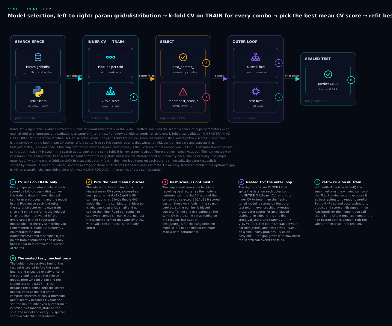
Hold onto the reason step 3 exists even after all that careful cross-validation in step 2. Cross-validation is for selection, not for the final reported number. Every choice you make to maximize the CV score adapts to that score — so by the time you have picked the winner, the CV score of that winner is optimistic, for precisely the same reason a test set you tuned against is no longer a test set. The CV number chooses; the sealed test number reports. Keeping those two jobs in two different pools of data is the entire discipline, and the tools below are just efficient, automated ways to do step 2 without ever peeking at the vault.
GridSearchCV: exhaustive search over a grid
The most direct way to search is to list the values you care about for each hyperparameter and try every combination. That is GridSearchCV: you hand it an estimator, a dictionary mapping hyperparameter names to lists of values, and a cross-validation strategy, and it fits and scores every point on the grid, then hands you the winner refit on all your data. Here it tunes an RBF SVM’s two hyperparameters — C and gamma — inside a scaling pipeline, on the breast-cancer training set:
import pandas as pd
from sklearn.model_selection import GridSearchCV
from sklearn.pipeline import Pipeline
from sklearn.svm import SVC

pipe = Pipeline([("scaler", StandardScaler()), ("svc", SVC(kernel="rbf"))])
grid = {"svc__C":     [0.1, 1, 10, 100],
        "svc__gamma": [1e-3, 1e-2, 1e-1, 1]}
cv = StratifiedKFold(5, shuffle=True, random_state=0)

gs = GridSearchCV(pipe, grid, scoring="roc_auc", cv=cv, n_jobs=-1, refit=True)
gs.fit(Xtr, ytr)                                          # Xtr, ytr = breast-cancer TRAIN

print("best_params_:", gs.best_params_)
print(f"best_score_ (mean CV ROC-AUC) = {gs.best_score_:.4f}")
print(f"sealed test ROC-AUC (touched ONCE) = {gs.score(Xte, yte):.4f}")
best_params_: {'svc__C': 10, 'svc__gamma': 0.01}
best_score_ (mean CV ROC-AUC) = 0.9960
sealed test ROC-AUC (touched ONCE) = 0.9987
Four attributes carry everything a fitted search knows, and you will reach for all four:
| Attribute | Holds | Use it to |
|---|---|---|
best_params_ |
The winning hyperparameter dict | See what won; reproduce it elsewhere |
best_score_ |
Mean CV score of the winner | Compare searches — never report as test score |
best_estimator_ |
The winner, refit on all training data | Predict, or score on the sealed test |
cv_results_ |
Every combo’s per-fold and mean scores + timings | Read the whole landscape, not just the peak |
cv_results_ is the one beginners ignore and experts live in, because the shape of the score surface tells you where to search next. Turn it into a DataFrame and read the top few, or pivot it into the actual grid:
res = pd.DataFrame(gs.cv_results_)
print(res[["param_svc__C", "param_svc__gamma", "mean_test_score",
           "std_test_score", "rank_test_score"]]
      .sort_values("rank_test_score").head(4).to_string(index=False))
print(res.pivot_table(index="param_svc__C", columns="param_svc__gamma",
                      values="mean_test_score").round(3).to_string())
 param_svc__C  param_svc__gamma  mean_test_score  std_test_score  rank_test_score
         10.0             0.010         0.996006        0.005292                1
          1.0             0.010         0.995306        0.004412                2
         10.0             0.001         0.994593        0.004377                3
        100.0             0.001         0.994365        0.004310                4
param_svc__gamma  0.001  0.010  0.100  1.000
param_svc__C
0.1               0.984  0.988  0.984   0.95
1.0               0.990  0.995  0.990   0.95
10.0              0.995  0.996  0.986   0.95
100.0             0.994  0.992  0.985   0.95
Read the pivot like a topographic map. The good region is the middle — moderate C, gamma around 0.01 — and the whole right column (gamma=1) collapses to 0.95, an over-local model whose influence radius is too small. The winner at (C=10, gamma=0.01) sits on a broad plateau, not a lonely spike, which is reassuring: a peak surrounded by other good scores is a real optimum, while a peak surrounded by bad scores is often noise you would not reproduce. This is the single best reason to look past best_params_ at the full cv_results_.
The constructor arguments you will actually set:
| Argument | Default | What it controls |
|---|---|---|
estimator |
— | The model or Pipeline to tune |
param_grid |
— | dict (or list of dicts) of name → list of values |
scoring |
estimator’s .score |
The metric to optimize — set it deliberately |
cv |
5 |
Int or splitter; use a stratified, seeded splitter |
refit |
True |
Refit the winner on all data → enables best_estimator_, predict |
n_jobs |
None |
-1 uses all cores; the folds run in parallel |
return_train_score |
False |
Add train scores to cv_results_ to see the gap |
error_score |
np.nan |
What to record when a fit raises; set "raise" to debug |
Now the catch that defines grid search. Its cost is the product of the grid dimensions times the number of folds, and that product explodes. Our little 4×4 grid is 16 combinations, at 5 folds that is 80 fits — instant. But the brief’s example of a 4×4×5 grid is 80 combinations, and at 5 folds that is 400 model fits; add a fourth hyperparameter with 5 values and you are at 2000. Every hyperparameter you add multiplies the whole search:
| Grid | Combinations | × 5-fold CV | Feel |
|---|---|---|---|
| 4 × 4 | 16 | 80 fits | Instant |
| 4 × 4 × 5 | 80 | 400 fits | Seconds to a minute |
| 5 × 5 × 5 | 125 | 625 fits | A coffee |
| 6 × 6 × 6 × 6 | 1,296 | 6,480 fits | A long lunch |
| 10 × 10 × 10 × 10 | 10,000 | 50,000 fits | Overnight — and probably wasteful |
This curse of dimensionality in the search space is why grid search, for all its simplicity, is often the wrong first tool. Most of those thousands of fits explore combinations that were never going to win — and there is a smarter way to spend the same budget.
RandomizedSearchCV: sample, don’t enumerate
Grid search spends its budget evenly, including on the vast regions of the grid that are obviously bad. RandomizedSearchCV spends it randomly but proportionally: you give it distributions to sample from rather than lists to enumerate, and a budget n_iter of how many combinations to try. It draws n_iter random points from the space and cross-validates each. The insight — from Bergstra and Bengio’s 2012 result that random search beats grid search for the same budget — is that when only a few hyperparameters actually matter (which is usually), random sampling covers the important dimensions far more densely than a grid wastes points on the unimportant ones.
Demonstrate it directly. Take a bigger SVM grid — 6×6 = 36 combinations, 180 fits — and pit it against a randomized search that samples just 12 points (60 fits) from continuous log-uniform distributions over the same ranges:
from scipy.stats import loguniform
from sklearn.model_selection import RandomizedSearchCV

grid = {"svc__C": np.logspace(-2, 3, 6), "svc__gamma": np.logspace(-4, 1, 6)}
gs = GridSearchCV(pipe, grid, scoring="roc_auc", cv=cv, n_jobs=-1).fit(Xtr, ytr)

dists = {"svc__C": loguniform(1e-2, 1e3), "svc__gamma": loguniform(1e-4, 1e1)}
rs = RandomizedSearchCV(pipe, dists, n_iter=12, scoring="roc_auc",
                        cv=cv, n_jobs=-1, random_state=0).fit(Xtr, ytr)

print(f"GridSearchCV      fits=180  best CV={gs.best_score_:.4f}  test={gs.score(Xte, yte):.4f}")
print(f"RandomizedSearch  fits= 60  best CV={rs.best_score_:.4f}  test={rs.score(Xte, yte):.4f}")
for n in (6, 12, 24):
    r = RandomizedSearchCV(pipe, dists, n_iter=n, scoring="roc_auc",
                           cv=cv, n_jobs=-1, random_state=0).fit(Xtr, ytr)
    print(f"n_iter={n:2d}  fits={n*5:3d}  best CV={r.best_score_:.4f}  test={r.score(Xte, yte):.4f}")
GridSearchCV      fits=180  best CV=0.9960  test=0.9987
RandomizedSearch  fits= 60  best CV=0.9908  test=0.9922
n_iter= 6  fits= 30  best CV=0.9908  test=0.9922
n_iter=12  fits= 60  best CV=0.9908  test=0.9922
n_iter=24  fits=120  best CV=0.9962  test=0.9985
Read the fits-versus-score table, because it is the whole argument for randomized search:
| Method | Fits | Best CV ROC-AUC | Sealed test | Fraction of grid’s fits |
|---|---|---|---|---|
| GridSearchCV (6×6) | 180 | 0.9960 | 0.9987 | 100% |
RandomizedSearchCV n_iter=6 |
30 | 0.9908 | 0.9922 | 17% |
RandomizedSearchCV n_iter=12 |
60 | 0.9908 | 0.9922 | 33% |
RandomizedSearchCV n_iter=24 |
120 | 0.9962 | 0.9985 | 67% |
With 17% of the fits, random search lands within 0.006 test ROC-AUC of the exhaustive grid; with 67% it ties it (0.9985 vs 0.9987, a difference that is pure noise). That is the bargain: near-best answers for a fraction of the compute, and — crucially — a budget you set with n_iter rather than one dictated by the grid’s dimensions. You want the search to run for an hour? Set n_iter to whatever fits in an hour. Grid search offers no such dial; you either run the whole grid or you do not.
The distributions are the new idea, and choosing them well is most of the skill. Use scipy’s continuous distributions, and mind the scale — regularization and learning rates live on a log scale, so sample them log-uniformly, not uniformly:
| Hyperparameter kind | Distribution | Why |
|---|---|---|
C, gamma, learning_rate, alpha |
loguniform(1e-4, 1e2) |
Orders of magnitude matter; uniform would over-sample the large end |
n_estimators, max_depth (int) |
randint(50, 500) |
Discrete counts, sampled uniformly |
subsample, max_features (fraction) |
uniform(0.5, 0.5) → [0.5, 1.0] |
Genuinely linear quantities |
| A small set of choices | a plain list |
Random search accepts lists too, and samples them |
RandomizedSearchCV shares every attribute and argument with GridSearchCV — best_params_, best_estimator_, cv_results_, refit, scoring, n_jobs — and adds two: n_iter (the budget) and random_state (so the same random points are drawn every run, which you must pin for reproducibility). The practical rule that falls out of all this: reach for randomized search first, especially with three or more hyperparameters, and only fall back to a grid when the space is small and you truly want every corner checked.
Successive halving and Bayesian search
Both searches so far give every candidate the same full cross-validation, even the obvious losers. Successive halving refuses to: it starts all candidates on a small slice of the data (or a few trees, a few iterations), throws out the worst fraction, and promotes the survivors to a larger slice — repeating until a few finalists are evaluated on the full budget. Cheap eliminations early, expensive evaluation only for contenders. scikit-learn ships HalvingGridSearchCV and HalvingRandomSearchCV, still behind an experimental import:
from sklearn.datasets import make_classification
from sklearn.experimental import enable_halving_search_cv   # noqa: F401 — required import
from sklearn.model_selection import HalvingGridSearchCV
from sklearn.ensemble import RandomForestClassifier

Xr, yr = make_classification(n_samples=3000, n_features=20, n_informative=8,
                             weights=[0.7], random_state=0)
Xrf_tr, _, yrf_tr, _ = train_test_split(Xr, yr, test_size=0.25, stratify=yr, random_state=0)

rf = RandomForestClassifier(random_state=0)
grid = {"n_estimators": [50, 100, 200], "max_depth": [3, 5, 8, None],
        "min_samples_leaf": [1, 5, 20]}                       # 3×4×3 = 36 combos

hs = HalvingGridSearchCV(rf, grid, scoring="f1", cv=cv, factor=3,
                         random_state=0, n_jobs=-1).fit(Xrf_tr, yrf_tr)
print("best CV F1 =", round(hs.best_score_, 3))
print("candidates per iteration:", list(hs.n_candidates_))
print("resources (samples) per iteration:", list(hs.n_resources_))
best CV F1 = 0.907
candidates per iteration: [36, 12, 4, 2]
resources (samples) per iteration: [83, 249, 747, 2241]
The schedule is the algorithm, laid bare:
| Iteration | Candidates | Resources (samples) | What happens |
|---|---|---|---|
| 0 | 36 | 83 | All candidates on the cheapest data slice |
| 1 | 12 | 249 | Keep the best 1/3, triple their data |
| 2 | 4 | 747 | Keep the best 1/3 again |
| 3 | 2 | 2,241 | Two finalists on (nearly) all the data |
36 candidates each get 83 samples; the best third (12) advance to 249 samples; then 4 to 747; then the 2 finalists to 2241. With factor=3, each round keeps 1/3 of the candidates and triples their data, so the expensive full-data fits happen only for the two survivors instead of all thirty-six. Against a plain GridSearchCV on the same grid it reached an essentially identical F1 (0.907 versus the grid’s 0.912) — and picked a slightly different winner, a reminder that halving is an approximation: a candidate that would have won on full data can occasionally be eliminated early on a small, unlucky slice. That is the price of the speed.
The landscape of search strategies, from dumbest-but-thorough to smartest-but-fiddliest:
| Strategy | How it explores | Best when | Cost |
|---|---|---|---|
GridSearchCV |
Every combination | Small space, want exhaustiveness | Product of dims — explodes |
RandomizedSearchCV |
n_iter random samples |
3+ hyperparameters; a fixed budget | You set it via n_iter |
HalvingGridSearchCV |
Grid + successive halving | Big grid, cheap-to-subsample data | Much less than full grid |
HalvingRandomSearchCV |
Random + successive halving | Large space and tight budget | The cheapest of the four |
Bayesian (Optuna, scikit-optimize) |
Model where to look next from past trials | Expensive fits, want few of them | Extra library; sequential |
That last row points beyond scikit-learn. Bayesian optimization — the popular library is Optuna, with scikit-optimize and hyperopt as alternatives — treats tuning as an optimization problem in its own right: it builds a probabilistic model of “score as a function of hyperparameters” from the trials so far and uses it to propose the next combination most likely to improve, rather than sampling blindly. In practice you write an objective(trial) function that asks the trial for values — trial.suggest_float("C", 1e-4, 1e2, log=True) — builds the estimator, and returns a cross_val_score(...).mean(); then study.optimize(objective, n_trials=50) runs the search, each trial informed by the last. When each fit is expensive — a deep network, a gradient-boosting model on millions of rows — spending a little compute to choose the next trial wisely pays for itself many times over. For the small, fast models in this course, randomized or halving search is plenty; file “Optuna” under the tool you reach for when a single fit takes minutes and you can afford only fifty of them.
Tuning inside a Pipeline: the real-world pattern
Here is where tuning stops being a toy and becomes the thing you actually do at work. Real problems do not just tune a model — they tune the preprocessing and the model together, because the best amount of feature selection depends on the model and vice versa. A Pipeline makes this not only possible but leakage-safe by construction, and the syntax is the one new thing to learn: address a step’s hyperparameter as stepname__paramname, with a double underscore.
Build a three-step pipeline — scale, select the k best features, classify — and tune the selector’s k and the classifier’s C in one search. Because SelectKBest lives inside the pipeline, it is refit on each fold’s training rows only, so choosing k by peeking at every label — the feature-selection leakage that inflated a pure-noise model to 0.865 in the evaluation lesson — cannot happen here:
from sklearn.feature_selection import SelectKBest, f_classif

pipe = Pipeline([
    ("scaler", StandardScaler()),
    ("select", SelectKBest(f_classif)),
    ("clf",    LogisticRegression(max_iter=5000)),
])
grid = {"select__k": [5, 10, 20, 30],        # a PREPROCESSING hyperparameter
        "clf__C":    [0.01, 0.1, 1, 10]}      # a MODEL hyperparameter
gs = GridSearchCV(pipe, grid, scoring="roc_auc", cv=cv, n_jobs=-1).fit(Xtr, ytr)

print("best_params_ (preprocessing AND model together):", gs.best_params_)
print(f"best CV ROC-AUC     = {gs.best_score_:.4f}")
print(f"sealed test ROC-AUC = {gs.score(Xte, yte):.4f}")
print(pd.DataFrame(gs.cv_results_).pivot_table(
      index="param_select__k", columns="param_clf__C",
      values="mean_test_score").round(4).to_string())
best_params_ (preprocessing AND model together): {'clf__C': 10, 'select__k': 20}
best CV ROC-AUC     = 0.9971
sealed test ROC-AUC = 0.9958
param_clf__C      0.01    0.10    1.00    10.00
param_select__k
5                0.9873  0.9873  0.9880  0.9870
10               0.9866  0.9871  0.9880  0.9882
20               0.9900  0.9946  0.9960  0.9971
30               0.9918  0.9953  0.9945  0.9844
The pivot shows the two hyperparameters interacting, which is exactly why you must tune them jointly rather than one at a time. At k=20 more regularization-relaxation helps (C=10 wins), but at k=30 — all features in — C=10 overfits and the score drops to 0.9844 while a gentler C=0.1 does best. Tune C alone at fixed k, or k alone at fixed C, and you would miss the joint optimum at (k=20, C=10). The grid found it because it searched the plane, not two lines.
To know what you can address with step__param, ask the pipeline for its parameter names:
print([p for p in pipe.get_params() if "__" in p][:8])
# ['scaler__copy', 'scaler__with_mean', 'scaler__with_std', 'select__k',
#  'select__score_func', 'clf__C', 'clf__class_weight', 'clf__dual']
| You want to tune… | Grid key | Reaches |
|---|---|---|
| Features kept by the selector | "select__k" |
SelectKBest(k=…) |
| Classifier regularization | "clf__C" |
LogisticRegression(C=…) |
| Whether the scaler centres | "scaler__with_mean" |
StandardScaler(with_mean=…) |
| Swap the whole model | "clf" |
Pass a list of estimators as the value |
That last row is a genuinely powerful trick: because a pipeline step is itself a hyperparameter, you can put estimators in the grid — {"clf": [LogisticRegression(...), RandomForestClassifier(...)]} — and let the search choose the algorithm alongside its hyperparameters, all in one leakage-safe cross-validation. This is the real-world pattern the preprocessing lesson was building toward: the pipeline is not a convenience for tidy code, it is the object that makes joint tuning of preprocessing and model honest.
Nested cross-validation: the honest estimate
Now the subtle, critical point that separates a careful practitioner from a fooled one — and the reason the red node sits in the middle of the diagram. When you run a search and read off best_score_, you are looking at the cross-validated score of the combination you selected because it had the best cross-validated score. That is circular, and the circularity biases the number upward. The search tried many combinations against the same folds and reported the luckiest; some of that luck is real signal, but some is just favourable noise in those particular folds, and noise does not generalize. Reporting best_score_ as your model’s performance is the same sin as tuning on the test set, only quieter.
The honest fix is nested cross-validation: two loops. An inner loop does the tuning (a full GridSearchCV), and an outer loop evaluates the tuned result on data the inner loop never saw. Each outer fold holds out a slice, the inner search tunes on the rest, and the freshly tuned model is scored on the held-out slice it never influenced. Average the outer scores and you have an estimate with the selection bias removed. In scikit-learn it is astonishingly little code — you cross_val_score a GridSearchCV:
# a small, noisy problem — plenty of room for the search to get lucky
Xn, yn = make_classification(n_samples=300, n_features=30, n_informative=4,
                             n_redundant=2, flip_y=0.12, class_sep=0.6, random_state=11)
inner = StratifiedKFold(5, shuffle=True, random_state=1)
outer = StratifiedKFold(5, shuffle=True, random_state=2)
grid  = {"svc__C": np.logspace(-1, 4, 7), "svc__gamma": np.logspace(-5, 1, 7)}

# FLAT: tune and read best_score_ off the SAME cv — optimistic
flat = GridSearchCV(pipe, grid, scoring="roc_auc", cv=inner, n_jobs=-1).fit(Xn, yn)

# NESTED: the outer loop scores a GridSearchCV whose inner loop does the tuning
search = GridSearchCV(pipe, grid, scoring="roc_auc", cv=inner, n_jobs=-1)
nested = cross_val_score(search, Xn, yn, scoring="roc_auc", cv=outer, n_jobs=-1)

print(f"FLAT   best_score_    = {flat.best_score_:.4f}   <- optimistic")
print(f"NESTED outer mean     = {nested.mean():.4f} ± {nested.std():.4f}  <- honest")
print(f"optimism gap          = {flat.best_score_ - nested.mean():+.4f}")
On a small, noisy problem (300 rows, a 7×7 grid — plenty of room for the search to get lucky) the gap is stark:
FLAT   best_score_    = 0.7199   <- optimistic
NESTED outer mean     = 0.6713 ± 0.0207  <- honest
optimism gap          = +0.0487
Nearly five points of pure self-deception. The flat search would let you promise 0.72; the honest, selection-unbiased estimate is 0.67. If you shipped on the strength of the 0.72, production would hand you the 0.67 and you would not understand why. But — and this is the nuance that makes the concept click — the size of the gap depends entirely on how much the search can overfit the folds. Run the identical experiment on the easy, saturated breast-cancer problem and the gap essentially vanishes:
| Dataset (grid) | Flat best_score_ |
Nested (honest) | Optimism gap |
|---|---|---|---|
| Tiny, noisy — n=300, 7×7 grid | 0.7199 | 0.6713 ± 0.021 | +0.0487 |
| Small, noisy — n=400, 6×6 grid | 0.7816 | 0.7642 ± 0.026 | +0.0174 |
| Breast cancer — n=569, 5×5 grid | 0.9960 | 0.9960 ± 0.005 | −0.0000 |
The pattern is the lesson: the optimism grows with the noise, the smallness of the data, and the size of the grid — every one of which gives the search more room to find a fold-specific fluke. On easy, abundant data with a modest grid there is little to overfit and flat CV is nearly honest; on hard, scarce data with a big search it lies by five points.
So when do you pay for nested CV’s extra loop? It is expensive — outer folds times the entire inner search — so you do not run it every time. You run it when you need to report an honest estimate of a tuned model’s performance and you cannot spare a separate test set (small data), or when you are comparing tuning procedures and need each one’s honest score. For everyday work, the sealed test set from the workflow is your outer loop: tune with CV on train, report once on test. Nested CV is what you use when you have no such vault to draw on, or when a reviewer asks “but is that number honest?” and you need to prove it.
| Flat CV (tune + report on same CV) | Nested CV (inner tunes, outer reports) | |
|---|---|---|
| What it estimates | Biased — the selection peeked | Unbiased — outer never influenced tuning |
| Cost | One search | Outer folds × one full search each |
Report best_score_? |
No — optimistic | The outer mean is the honest number |
| Use when | Choosing between models/params | Reporting honest performance on small data |
Validation curves and learning curves
Two diagnostic plots turn tuning from guesswork into reading, and they answer two different questions. A validation curve varies one hyperparameter and plots training and validation score against it — it shows you where under- and overfitting live along that axis. A learning curve varies the training-set size and plots the two scores against it — it shows you whether more data would help. Confusing them is common; the axes are different and so are the cures.
Start with the validation curve, sweeping an SVM’s C across seven orders of magnitude:
from sklearn.model_selection import validation_curve
pipe = Pipeline([("scaler", StandardScaler()), ("svc", SVC(kernel="rbf", gamma=0.01))])
C_range = np.logspace(-3, 3, 7)
tr, va = validation_curve(pipe, X, y, param_name="svc__C", param_range=C_range,
                          cv=cv, scoring="roc_auc")
print("C        :", " ".join(f"{c:8.3g}" for c in C_range))
print("train AUC:", " ".join(f"{v:8.3f}" for v in tr.mean(1)))
print("valid AUC:", " ".join(f"{v:8.3f}" for v in va.mean(1)))
C        :    0.001     0.01      0.1        1       10      100    1e+03
train AUC:    0.987    0.987    0.991    0.996    0.998    1.000    1.000
valid AUC:    0.986    0.987    0.991    0.995    0.996    0.994    0.990
Read it left to right as a story about capacity. At tiny C the model is heavily regularized and slightly underfit — train and validation are low and together (0.987 / 0.986). As C grows the model gains capacity and both scores rise, until validation peaks at C=10 (0.996). Past that, train marches on to a perfect 1.000 while validation falls to 0.990 — the model is spending its new capacity memorizing, and the widening train-minus-validation gap is overfitting made visible. The best C is the one that maximizes validation, not train — here, 10 — and the curve shows you not just the answer but the shape of the tradeoff around it.
| Region of a validation curve | Train | Validation | Gap | Meaning |
|---|---|---|---|---|
| Hyperparameter too “small” | Low | Low | Small | Underfit — not enough capacity |
| At the validation peak | High | Highest | Small–moderate | The value to choose |
| Hyperparameter too “large” | Very high → 1.0 | Falling | Widening | Overfit — capacity spent memorizing |
Now the learning curve, which fixes the hyperparameters and grows the data instead:
from sklearn.model_selection import learning_curve
sizes, tr, va = learning_curve(
    Pipeline([("scaler", StandardScaler()), ("svc", SVC(kernel="rbf", C=10, gamma=0.01))]),
    X, y, cv=cv, scoring="roc_auc",
    train_sizes=np.linspace(0.1, 1.0, 6), random_state=0)
print("train size:", " ".join(f"{int(s):5d}" for s in sizes))
print("train AUC :", " ".join(f"{v:5.3f}" for v in tr.mean(1)))
print("valid AUC :", " ".join(f"{v:5.3f}" for v in va.mean(1)))
train size:    45   127   209   291   373   455
train AUC : 0.999 0.999 1.000 0.998 0.998 0.998
valid AUC : 0.984 0.992 0.994 0.995 0.995 0.996
The train score is flat and near-perfect; the validation score climbs from 0.984 at 45 samples to 0.996 at 455 as the gap narrows from 0.015 to 0.002. The two curves are converging and beginning to plateau — validation has nearly caught up to train and is levelling off — which is the signature of a model that has about enough data. If the two curves were still racing toward each other with a wide gap at the right edge, more data would clearly help; if they had met at a low score, you would be underfitting and more data would be useless — you would need a richer model instead. That single question, would more data help?, is what only a learning curve can answer, and it is often worth more than any hyperparameter.
| Curve | X-axis | Diagnoses | Cure it points to |
|---|---|---|---|
| Validation curve | One hyperparameter | Under/overfit along that knob | Set the knob to the validation peak |
| Learning curve | Training-set size | Whether more data would help | Gather data (converging, high) or enrich the model (converged, low) |
The practical reality of tuning
Everything above is mechanism; this section is judgment, and judgment is what keeps you from burning a weekend of compute for a 0.001 gain. A handful of hard-won rules.
Go coarse, then fine. Do not start with a dense grid over a narrow range — you do not yet know where the good region is. Start with a wide, coarse search (log-spaced, a few points per decade), find the neighbourhood of the best score, then run a second, finer search zoomed into that neighbourhood. Concretely: a first pass over C = np.logspace(-3, 3, 7) might peak at C=10; the second pass then searches C = [3, 5, 10, 30, 50] around that winner. Two cheap searches beat one enormous one, and the coarse pass tells you whether you are even in the right range before you spend on precision — if the peak sits at the edge of your coarse range, extend the range rather than refining, because the real optimum is probably still outside it.
Do not tune everything. Most hyperparameters barely move the score; a few dominate. For an SVM it is C and gamma; for gradient boosting, learning_rate and n_estimators and max_depth; for a random forest, honestly, the defaults are hard to beat and max_depth/min_samples_leaf are where the leverage is. Tuning ten hyperparameters when two matter multiplies your search cost by orders of magnitude to explore noise. Identify the two or three that matter — the capacity dials — and tune those.
Respect diminishing returns and a compute budget. The first coarse search often captures most of the available gain; the second, refined one adds a little; a third adds almost nothing. Decide your budget before you start — “this search runs overnight, no more” — and let n_iter or a halving schedule fit the work to the budget rather than letting an exhaustive grid dictate a week. A model that is 0.001 better after eight more hours of tuning is not better in any way your users will notice.
And the rule that outranks all the others: better features and more data beat better hyperparameters. This is the honest, slightly deflating truth of applied machine learning. The gap between default and perfectly-tuned hyperparameters is usually a few percent; the gap between mediocre features and good ones, or between a thousand rows and a hundred thousand, is often the whole game. If your model is not good enough, your first instinct should be a better feature or more data, not a bigger grid — tuning is the polish you apply to a model that is already fundamentally sound, not the thing that makes an unsound one work. A learning curve that is still climbing steeply is telling you to go get data, not to tune harder.
| Symptom | The tempting move | The move that usually wins |
|---|---|---|
| Model underperforms | Tune harder, bigger grid | Better features; check the learning curve for “more data” |
| Learning curve still climbing | Tune the model | Gather more data |
| Learning curves converged, both low | More data | A richer model / new features (you are underfitting) |
| Gain of 0.001 after a huge search | Search even more | Stop — you have hit diminishing returns |
| Score unstable run to run | Trust the best run | Pin random_state; report mean ± std across seeds |
Finally, reproducibility, which threads through every example above. Three separate sources of randomness must be pinned or your results wander: the data split, the model’s own randomness, and the CV splitter. And one performance knob, n_jobs, has a cost worth knowing:
| Knob | Set it to | Why / the catch |
|---|---|---|
train_test_split(random_state=…) |
any fixed int | Same split every run |
model random_state=… (RF, trees, SGD) |
any fixed int | Same learned model |
CV splitter random_state=… (with shuffle=True) |
any fixed int | Same folds — so the search is reproducible |
RandomizedSearchCV(random_state=…) |
any fixed int | Same sampled combinations |
n_jobs=-1 |
all cores | Fits run in parallel — but each worker copies the data, so a big dataset × many cores can exhaust RAM; drop to n_jobs=4 if memory spikes |
Pin the first four and your entire search reproduces byte-for-byte; leave any one unpinned and “why did the score change?” becomes an unanswerable question mid-project.
Hands-on lab
One self-contained script, tune_lab.py. It builds a fresh imbalanced problem, seals a test set, tunes a scaling-plus-SVM pipeline with GridSearchCV (reading best_params_ and cv_results_), matches it with RandomizedSearchCV in a fraction of the fits, plots a validation curve and a learning curve headless, demonstrates the nested-versus-flat optimism gap, and finally unseals the test set exactly once. Every number below is from an actual run on scikit-learn 1.9.0.
Set up once:
python3 -m venv .venv
source .venv/bin/activate          # Windows: .venv\Scripts\activate
python -m pip install scikit-learn numpy pandas matplotlib scipy
Step 1 — a problem, a sealed test set, a pipeline
import numpy as np, matplotlib
matplotlib.use("Agg")                                  # headless: save, don't show
import matplotlib.pyplot as plt
import pandas as pd
from scipy.stats import loguniform
from sklearn.datasets import make_classification
from sklearn.model_selection import (train_test_split, GridSearchCV, RandomizedSearchCV,
                                     cross_val_score, validation_curve, learning_curve,
                                     StratifiedKFold)
from sklearn.pipeline import Pipeline
from sklearn.preprocessing import StandardScaler
from sklearn.svm import SVC

X, y = make_classification(n_samples=800, n_features=20, n_informative=6,
                           n_redundant=2, weights=[0.6], flip_y=0.06,
                           class_sep=0.9, random_state=42)
X_tr, X_te, y_tr, y_te = train_test_split(X, y, test_size=0.25, stratify=y, random_state=42)
pipe = Pipeline([("scaler", StandardScaler()), ("svc", SVC(kernel="rbf"))])
cv = StratifiedKFold(5, shuffle=True, random_state=0)
print(f"[1] train={len(y_tr)}  test={len(y_te)} (sealed)  positive rate={y.mean():.2f}")
[1] train=600 test=200 (sealed) positive rate=0.41
What just happened: the test set is sealed on line one and does not reappear until Step 7. Everything between tunes on the 600 training rows only.
Step 2 — GridSearchCV, reading best_params_ and cv_results_
grid = {"svc__C": [0.1, 1, 10, 100], "svc__gamma": [1e-3, 1e-2, 1e-1, 1]}
gs = GridSearchCV(pipe, grid, scoring="roc_auc", cv=cv, n_jobs=-1).fit(X_tr, y_tr)
print(f"[2] 16 combos × 5 folds = 80 fits")
print(f"    best_params_ = {gs.best_params_}")
print(f"    best_score_  = {gs.best_score_:.4f} (mean CV ROC-AUC)")
for _, r in pd.DataFrame(gs.cv_results_).sort_values("rank_test_score").head(3).iterrows():
    print(f"    rank {int(r['rank_test_score'])}: C={r['param_svc__C']:<5} "
          f"gamma={r['param_svc__gamma']:<6} CV={r['mean_test_score']:.4f} ± {r['std_test_score']:.4f}")
[2] 16 combos × 5 folds = 80 fits
    best_params_ = {'svc__C': 100, 'svc__gamma': 0.01}
    best_score_  = 0.8876 (mean CV ROC-AUC)
    rank 1: C=100.0 gamma=0.01   CV=0.8876 ± 0.0129
    rank 2: C=10.0  gamma=0.01   CV=0.8833 ± 0.0275
    rank 3: C=10.0  gamma=0.1    CV=0.8724 ± 0.0239
What just happened: the grid found (C=100, gamma=0.01) at CV ROC-AUC 0.888. Note rank 2’s ± 0.0275 is twice rank 1’s spread — the winner is not just higher, it is steadier, which matters as much as the mean.
Step 3 — RandomizedSearchCV, the same answer for fewer fits
dists = {"svc__C": loguniform(1e-1, 1e2), "svc__gamma": loguniform(1e-3, 1e0)}
print(f"    {'method':<24}{'fits':>5}{'best CV':>10}")
print(f"    {'GridSearchCV':<24}{80:>5}{gs.best_score_:>10.4f}")
for n in (5, 8, 12):
    rs = RandomizedSearchCV(pipe, dists, n_iter=n, scoring="roc_auc",
                            cv=cv, n_jobs=-1, random_state=0).fit(X_tr, y_tr)
    print(f"    {'RandomizedSearchCV n='+str(n):<24}{n*5:>5}{rs.best_score_:>10.4f}")
    method                   fits   best CV
    GridSearchCV               80    0.8876
    RandomizedSearchCV n=5     25    0.8859
    RandomizedSearchCV n=8     40    0.8859
    RandomizedSearchCV n=12    60    0.8859
What just happened: with 25 fits — under a third of the grid’s 80 — random search is within 0.002 ROC-AUC of the exhaustive answer. On a real problem where each fit costs minutes, that is the difference between an afternoon and a coffee.
Step 4 — a validation curve over C
C_range = np.logspace(-2, 3, 6)
tr, va = validation_curve(Pipeline([("scaler", StandardScaler()),
                                    ("svc", SVC(kernel="rbf", gamma=0.01))]),
                          X_tr, y_tr, param_name="svc__C", param_range=C_range,
                          cv=cv, scoring="roc_auc")
print("[4] C        :", " ".join(f"{c:7.3g}" for c in C_range))
print("    train AUC:", " ".join(f"{v:7.3f}" for v in tr.mean(1)))
print("    valid AUC:", " ".join(f"{v:7.3f}" for v in va.mean(1)))
[4] C        :    0.01     0.1       1      10     100   1e+03
    train AUC:   0.854   0.854   0.889   0.962   0.995   1.000
    valid AUC:   0.825   0.825   0.845   0.883   0.888   0.859
What just happened: validation peaks at C=100 (0.888) then falls to 0.859 at C=1000 even as train hits a perfect 1.000 — textbook overfitting past the peak. The grid in Step 2 was right to stop at 100.
Step 5 — a learning curve
sizes, ltr, lva = learning_curve(gs.best_estimator_, X_tr, y_tr, cv=cv, scoring="roc_auc",
                                 train_sizes=np.linspace(0.1, 1.0, 6), random_state=0)
print("[5] size     :", " ".join(f"{int(s):7d}" for s in sizes))
print("    train AUC:", " ".join(f"{v:7.3f}" for v in ltr.mean(1)))
print("    valid AUC:", " ".join(f"{v:7.3f}" for v in lva.mean(1)))

fig, (a1, a2) = plt.subplots(1, 2, figsize=(11, 4.5), layout="constrained")
a1.semilogx(C_range, tr.mean(1), "o-", label="train"); a1.semilogx(C_range, va.mean(1), "o-", label="validation")
a1.set(title="Validation curve (C)", xlabel="svc__C", ylabel="ROC-AUC"); a1.legend()
a2.plot(sizes, ltr.mean(1), "o-", label="train"); a2.plot(sizes, lva.mean(1), "o-", label="validation")
a2.set(title="Learning curve", xlabel="training samples", ylabel="ROC-AUC"); a2.legend()
fig.savefig("tune_curves.png", dpi=120, bbox_inches="tight")
print("    wrote tune_curves.png")
[5] size     :      48     134     220     307     393     480
    train AUC:   1.000   1.000   1.000   0.998   0.998   0.995
    valid AUC:   0.742   0.816   0.830   0.858   0.871   0.888
    wrote tune_curves.png
What just happened: validation climbs steadily from 0.742 to 0.888 as data grows, and the train-minus-validation gap is still a wide ~0.11 at the right edge. The curves have not converged — this model would genuinely benefit from more data, the most valuable thing a learning curve can tell you.
Step 6 — nested vs flat CV, the optimism gap
inner = StratifiedKFold(5, shuffle=True, random_state=1)
outer = StratifiedKFold(5, shuffle=True, random_state=2)
flat = GridSearchCV(pipe, grid, scoring="roc_auc", cv=inner, n_jobs=-1).fit(X_tr, y_tr)
nested = cross_val_score(GridSearchCV(pipe, grid, scoring="roc_auc", cv=inner, n_jobs=-1),
                         X_tr, y_tr, scoring="roc_auc", cv=outer, n_jobs=-1)
print(f"[6] FLAT   best_score_ = {flat.best_score_:.4f}  <- tempting to report")
print(f"    NESTED outer mean  = {nested.mean():.4f} ± {nested.std():.4f}  <- honest")
print(f"    optimism gap       = {flat.best_score_ - nested.mean():+.4f}")
[6] FLAT   best_score_ = 0.8912  <- tempting to report
    NESTED outer mean  = 0.8840 ± 0.0219  <- honest
    optimism gap       = +0.0072
What just happened: the flat search’s best_score_ is 0.007 optimistic versus the nested estimate — modest here because the problem is not tiny, but real and always in the same direction: up.
Step 7 — unseal the test set, exactly once
print(f"[7] chosen model {gs.best_params_}")
print(f"    CV said {gs.best_score_:.4f}   sealed test says {gs.score(X_te, y_te):.4f}")
[7] chosen model {'svc__C': 100, 'svc__gamma': 0.01}
    CV said 0.8876   sealed test says 0.8766
What just happened: the final, honest number is 0.877 — close to the CV estimate of 0.888 because the pipeline kept the whole search leakage-free. That single test evaluation is the only time X_te was touched, and now the lab is done. Report 0.877, not 0.888, and never re-open the test set to “improve” things.
⚠️ The
gs.score(X_te, y_te)call is your one permitted look at the test set. Run it in a loop while tweaking the grid and you have silently converted your test set into a validation set — every subsequent number is fiction.
Common mistakes and troubleshooting
| Symptom / message | Cause | Fix |
|---|---|---|
AttributeError: This 'GridSearchCV' has no attribute 'predict' |
Called .predict with refit=False |
Leave refit=True (default), or refit manually from best_params_ |
AttributeError: 'GridSearchCV' object has no attribute 'best_estimator_' |
refit=False then read best_estimator_ |
Same — refit must be truthy to expose the winner |
InvalidParameterError: The 'scoring' parameter … Got 'rock_auc' instead. |
Misspelled scoring string | Use a valid name: "roc_auc", "f1", "average_precision", … |
ValueError: Invalid parameter 'C' for estimator Pipeline(...) |
Grid key missing the step__ prefix |
Address pipeline params as "svc__C", not "C" |
| CV score high, sealed-test / production much lower | Flat-CV optimism — reported best_score_ |
Report the sealed-test score; for small data use nested CV |
| Search runs for hours | Grid too big (combinatorial blow-up) | RandomizedSearchCV / halving; coarse-then-fine; tune fewer knobs |
| Pipeline-less search beats the Pipeline version | Preprocessing leakage — scaler/selector fit on all data | Put every preprocessing step inside the tuned Pipeline |
UndefinedMetricWarning: … ill-defined during search |
A fold predicted no positives for precision/f1 |
Wrong scoring for imbalance — use average_precision/roc_auc; or accept zero_division |
best_params_ different every run |
random_state unset on split / model / CV / search |
Pin all four random_states |
RAM spikes / machine swaps with n_jobs=-1 |
Each parallel worker copies the dataset | Lower to n_jobs=4; or shrink the data per fit |
| Tuned for an hour, model no better | Saturated model — diminishing returns | Stop; invest in features/data (check the learning curve) |
FutureWarning: 'penalty' was deprecated in version 1.8 |
Set LogisticRegression(penalty=…) (removed in 1.10) |
Use C / l1_ratio instead; leave penalty at its default |
cv=5 gives weird folds on ordered data |
Bare int → unshuffled StratifiedKFold |
Pass StratifiedKFold(5, shuffle=True, random_state=0) |
Three of these deserve a longer look, because they are the ones that quietly corrupt results rather than loudly crashing.
Tuning without a Pipeline reintroduces the leakage you thought you’d escaped. It is tempting to StandardScaler().fit_transform(X) once, up front, and then run GridSearchCV on the scaled array — it looks cleaner. It is also leakage: the scaler learned its mean and standard deviation from all the data, including the rows that become each fold’s validation slice, so every CV score in the search is contaminated. Worse, the contamination is invisible — the search machinery runs perfectly on poisoned inputs and reports honest-looking numbers about a dishonest setup. The only fix is structural: put the scaler inside the estimator you hand to the search, so cross-validation refits it per fold on training rows only. This is the entire reason the preprocessing lesson insists preprocessing belongs inside the model, and it matters more during tuning, not less, because a search amplifies a small leak across hundreds of fits.
Reporting the CV score as the test score is the most common way tuned models disappoint. best_score_ is not your model’s performance; it is the performance of the luckiest combination you tried, measured on the folds it got lucky on. It is optimistic by construction — by five points on the small noisy problem above — and the optimism grows with grid size, noise, and data scarcity. Discipline: best_score_ is a selection number, used only to compare and choose; the number you report comes from the sealed test set (touched once) or, when you have no test set to spare, from the outer loop of a nested CV. If the only number you have is best_score_, you do not yet have an honest estimate of anything.
The wrong scoring optimizes for the wrong thing, silently. A search does exactly what you tell it: it maximizes scoring. Leave it at the default and a classifier optimizes accuracy — which, on the imbalanced data where tuning matters most, rewards a model that predicts the majority class and ignores the rare one you care about. The search will dutifully hand you the combination with the best accuracy, and it will be useless for catching fraud or disease. Choose scoring to match the cost of the errors you actually care about — average_precision or recall on imbalanced problems, neg_root_mean_squared_error when large regression errors are catastrophic — before you launch the search, because the search cannot know what you meant, only what you asked for.
Cheat-sheet
| Task | Code |
|---|---|
| Grid search a pipeline | GridSearchCV(pipe, grid, scoring="roc_auc", cv=cv, n_jobs=-1).fit(X_tr, y_tr) |
| Grid keys (pipeline step params) | {"svc__C": [1, 10], "svc__gamma": [0.01, 0.1]} |
| Randomized search | RandomizedSearchCV(pipe, dists, n_iter=30, cv=cv, random_state=0) |
| Log-scaled distribution | from scipy.stats import loguniform; loguniform(1e-4, 1e2) |
| Integer distribution | from scipy.stats import randint; randint(50, 500) |
| Successive halving | from sklearn.experimental import enable_halving_search_cv → HalvingRandomSearchCV(...) |
| Read the winner | search.best_params_, search.best_score_, search.best_estimator_ |
| Read the whole landscape | pd.DataFrame(search.cv_results_) |
| Predict with the tuned model | search.predict(X_new) (needs refit=True) |
| Score the sealed test once | search.score(X_te, y_te) |
| Tune model and preprocessing | {"select__k": [10, 20], "clf__C": [0.1, 1]} |
| Swap the model itself | {"clf": [LogisticRegression(), RandomForestClassifier()]} |
| Cross-validate (select) | cross_val_score(pipe, X, y, cv=StratifiedKFold(5, shuffle=True, random_state=0)) |
| Several metrics + train gap | cross_validate(pipe, X, y, cv=cv, scoring=[...], return_train_score=True) |
| Nested CV (honest estimate) | cross_val_score(GridSearchCV(pipe, grid, cv=inner), X, y, cv=outer) |
| Validation curve (one knob) | validation_curve(est, X, y, param_name="svc__C", param_range=..., cv=cv) |
| Learning curve (data size) | learning_curve(est, X, y, train_sizes=np.linspace(0.1,1,5), cv=cv) |
| Reproducibility | Pin random_state on split, model, CV splitter, and search |
| Budget knob | n_iter (randomized) or factor (halving) — fit the search to the clock |
Interview and exam questions
Q: What is the difference between a parameter and a hyperparameter?
A: A parameter is learned by fit from the data — the coefficients of a linear model, the splits of a tree — and lives in trailing-underscore attributes like coef_. A hyperparameter is set by you before fitting — C, max_depth, n_neighbors — and configures how learning happens; the model cannot learn it by ordinary fitting because it governs the fitting itself. Tuning is the search over hyperparameters.
Q: Why can’t you tune hyperparameters against a single train/validation split? A: Because a single split’s score depends on which rows landed where, and that noise is often larger than the effect you’re tuning. The same model varied by 0.010 across split seeds in this lesson — so a hyperparameter that moves the score by 0.005 is indistinguishable from luck. Cross-validation replaces the one lucky number with a mean ± std, and you only trust an improvement that clears the noise band.
Q: Walk through what GridSearchCV does, and name its four key attributes.
A: It enumerates every combination in the grid, runs k-fold CV on each, and (with refit=True) retrains the best combination on all the data. best_params_ is the winning dict, best_score_ is its mean CV score (for selection, never reporting), best_estimator_ is the winner refit on all training data and ready to predict, and cv_results_ holds every combination’s per-fold scores, means, stds, and timings.
Q: A 5×5×5 grid with 5-fold CV — how many model fits, and what’s the concern?
A: 125 combinations × 5 folds = 625 fits. The concern is the combinatorial blow-up: each hyperparameter you add multiplies the total, so grid search scales terribly. The fixes are RandomizedSearchCV (sample n_iter points and set your own budget), successive halving (eliminate weak candidates cheaply on small data slices), a coarse-then-fine strategy, and simply tuning fewer hyperparameters.
Q: When does RandomizedSearchCV beat GridSearchCV, and why?
A: Almost always with three or more hyperparameters. When only a few hyperparameters matter — the usual case — random sampling covers those important dimensions far more densely than a grid, which wastes points enumerating the unimportant ones. In this lesson random search reached within 0.006 test ROC-AUC of the full grid using 17% of the fits, and tied it with 67%. It also lets you set the budget directly via n_iter.
Q: What is nested cross-validation, and what problem does it solve?
A: It’s two CV loops — an inner loop that tunes (a full GridSearchCV) and an outer loop that scores each tuned model on data the inner loop never saw. It solves the optimism of flat CV: best_score_ is the score of the combination selected because it scored best on those folds, so it’s biased upward. The outer loop’s average is an unbiased estimate. In sklearn: cross_val_score(GridSearchCV(...), X, y, cv=outer).
Q: How big is the flat-CV optimism, and what makes it bigger? A: It varies from essentially zero to several points. On an easy, saturated problem the gap was −0.000; on a small, noisy problem with a big grid it was +0.049 ROC-AUC — five points of self-deception. The gap grows with anything that gives the search more room to overfit the folds: more noise, less data, and a larger grid. It is always in the same direction — the flat score is too high.
Q: You have a pipeline [scaler, select, clf]. Write a grid that tunes the number of selected features and the classifier’s C together, and explain why the pipeline makes it safe.
A:
grid = {"select__k": [5, 10, 20], "clf__C": [0.1, 1, 10]}
GridSearchCV(pipe, grid, scoring="roc_auc", cv=cv).fit(X_tr, y_tr)
The step__param double-underscore syntax addresses each step’s hyperparameter. It’s leakage-safe because SelectKBest lives inside the pipeline: on every fold, cross-validation refits the selector on that fold’s training rows only, so choosing k never peeks at the validation labels — the feature-selection leakage that can manufacture a strong score from pure noise is structurally impossible.
Q: What’s the difference between a validation curve and a learning curve? A: A validation curve varies one hyperparameter and plots train/validation score against it — it shows under/overfitting along that knob, and you pick the value at the validation peak. A learning curve varies the training-set size and plots the scores against it — it answers “would more data help?” If the curves are still converging with a wide gap, gather data; if they’ve met at a low score, you’re underfitting and need a richer model instead.
Q: You call search.predict(X) and get AttributeError: This 'GridSearchCV' has no attribute 'predict'. Why?
A: The search was created with refit=False, so it never retrained the winning combination and has no model to predict with — best_estimator_, predict, and score all become unavailable. Fix it by leaving refit=True (the default), which refits the winner on all the training data, or refit an estimator yourself from best_params_.
Q: Your tuned model gained 0.001 after an eight-hour search. What do you conclude? A: You’ve hit diminishing returns on a probably-saturated model, and more tuning is wasted effort. The honest next move is not a bigger grid but better features or more data — the gap between default and perfectly-tuned hyperparameters is usually a few percent, while better features or an order of magnitude more data is often the whole game. A learning curve tells you which: still climbing means get data; converged and low means enrich the model.
Q: Why must scoring be chosen deliberately before a search, especially on imbalanced data?
A: The search maximizes exactly scoring and nothing else. The default for classifiers is accuracy, which on imbalanced data rewards predicting the majority class — so the search will hand you a model that ignores the rare class you actually care about. Set scoring="average_precision" or "recall" for imbalanced positives, or "neg_root_mean_squared_error" for regression where big misses hurt, so the search optimizes what you mean rather than what the default assumes.
Key takeaways
- Parameters are learned by
fit; hyperparameters are set by you. Coefficients and tree splits are the output of training;C,max_depth, andn_estimatorsare the input that configures it. Tuning is the systematic search over the second kind — and nearly every hyperparameter is, at heart, a capacity dial on the underfit-to-overfit axis. - Cross-validation is the engine of selection, and a single number lies. Never tune against one split — its seed-to-seed noise drowns the signal. Report mean ± std, and treat two models as tied when their bands overlap; carry the spread through every decision.
- There is one honest workflow: seal the test set, search on train with CV, unseal the test once. Every decision — model, hyperparameters, threshold — is made by cross-validation on the training data. The test set comes out of the vault a single time, at the end, for the number you report, and then you stop.
GridSearchCVis exhaustive and explodes;RandomizedSearchCVis the better default. Grid cost is the product of the dimensions times the folds — a 4×4×5 grid is 400 fits. Random search samplesn_iterpoints from distributions, sets your budget directly, and reaches near-best answers for a fraction of the fits (17% here to get within 0.006). Successive halving and Bayesian tools (Optuna) go further when fits are expensive.- Tune preprocessing and model together, inside a Pipeline. The
step__paramsyntax tunes a selector’skand a classifier’sCin one search, and because the steps live inside the pipeline, cross-validation refits them per fold — joint tuning that is leakage-safe by construction. You can even put estimators in the grid to choose the algorithm too. - Flat CV’s
best_score_is optimistic; nested CV gives the honest estimate. Reporting the search’s own best CV score is the same sin as tuning on the test set — the number is biased up by however much the search could overfit the folds (+0.049 on a small noisy problem, ~0 on an easy one). Use the sealed test set, or the outer loop of a nested CV, for the number you actually quote. - Validation curves diagnose one knob; learning curves diagnose your data. A validation curve shows where a hyperparameter tips from underfit to overfit — pick the validation peak. A learning curve answers whether more data would help — the single most valuable question, and one no amount of tuning can address.
- Better features and more data beat better hyperparameters. Tuning is polish on a fundamentally sound model, not a rescue for an unsound one. Go coarse-then-fine, tune only the two or three knobs that matter, respect a compute budget and diminishing returns, pin every
random_state, and when the gain drops to a rounding error — stop, and go get better data instead.