You have heard that a neural network “works like the brain.” Forget that sentence — it has done more to mystify deep learning than any equation ever did. A neural network is three things you already half-know, chained together: a pile of weighted sums (linear algebra), a squish applied after each one (a nonlinear function), and a way to nudge the weights so the answer gets less wrong (calculus — the chain rule). That is the entire idea. No spark of cognition, no silicon neurons firing with intent. It is a function with a great many tunable knobs, and “training” is turning those knobs to fit examples.
The honest framing matters because it tells you exactly what to expect and what will break. The “brain” story predicts nothing; “chained linear algebra plus a nonlinearity plus gradient descent” predicts everything in this lesson — why depth needs that squish (without it, ten layers collapse into one), why a badly chosen step size makes the loss explode to infinity, why a neuron can quietly die and stop learning, and why the whole thing is just repeated arithmetic you can do in numpy without a single import from PyTorch or TensorFlow.
That last point is the design of this lesson. The next lesson hands you a framework — torch.nn, autograd, GPUs — and you will never hand-write a gradient again. So here, before the abstraction arrives, we build a real 2-layer network in pure numpy: the forward pass, the loss, the backward pass, and the update, all as arithmetic on arrays you can print and check. We will train it on XOR — the tiny problem that a single linear model provably cannot solve, but a one-hidden-layer net cracks in a few thousand steps — and you will watch the loss fall from 0.265 to 0.0002 and the predictions snap to the right answers. Every number on this page was executed on CPython 3.12 with numpy 2.x; run the code and you will get the same numbers.
You need only the scientific stack. Use a virtual environment — never pip install into the system Python:
python3 -m venv .venv
source .venv/bin/activate          # Windows: .venv\Scripts\activate
pip install numpy matplotlib
python -c "import numpy; print('numpy', numpy.__version__)"
# => numpy 2.5.1   (any recent 2.x — or 1.24+ — is fine)
This lesson assumes you are fluent with arrays — @ for matrix multiply, .T, broadcasting, axis=. If X @ W and a.sum(axis=0) are not yet reflex, read NumPy: Arrays, Broadcasting & Vectorization first, because a neural network is nothing but those operations in a loop. It also builds directly on ML Fundamentals: Supervised vs Unsupervised — a neural network is one more supervised model that learns f(X) ≈ y by minimizing a loss, so the X/y vocabulary, the train/test discipline, and the overfitting story from that lesson all still apply.
Why this matters
Machine learning, as the fundamentals lesson framed it, is learning a function from data instead of writing it by hand. Classical models — linear regression, a decision tree, KMeans — learn a simple, fixed shape of function. Linear regression can only ever fit a straight line (or flat plane); it is fast and interpretable, but if the true relationship curves, a line will always underfit it. You can bolt curves on by hand (polynomial features, interaction terms), but then you are back to guessing the shape.
A neural network’s pitch is different: stack enough simple nonlinear pieces and the network can approximate essentially any function, learning the shape itself from the data rather than being told it. This is not hand-waving — it is a theorem (the universal approximation theorem): a network with even a single hidden layer of enough neurons can approximate any continuous function to arbitrary accuracy. That flexibility is the whole appeal, and — exactly as the bias–variance story warns — it is also the whole danger. A model flexible enough to fit anything is flexible enough to memorize noise, so everything you learned about holding out data and watching the generalization gap matters more for neural nets, not less.
The catch that kept neural networks in the wilderness for decades was not the idea — it was the training. A network has thousands to billions of weights, and there is no closed-form equation for the best ones. The breakthrough (popularized in 1986, though invented earlier) was backpropagation: a way to compute, efficiently, how much each weight contributed to the error, so you can nudge them all in the right direction at once. Backprop is the beating heart of every deep-learning system on earth, and it is — this is the reassuring part — just the chain rule from calculus, applied backward through the layers. By the end of this lesson you will have written it by hand and confirmed it is correct against a numerical check. Once you have seen that it is only arithmetic, the mystique is gone for good, and the frameworks in the next lesson become a convenience rather than a black box.
Here is the map of what we build, one piece at a time, each verified in numpy:
| Piece | What it is | In one line |
|---|---|---|
| Neuron | a weighted sum plus a squish | a = activation(w·x + b) |
| Layer | many neurons in parallel | A = activation(X @ W + b) |
| Forward pass | run input → output | chain the layers left to right |
| Loss | one number: how wrong | MSE for numbers, cross-entropy for classes |
| Gradient descent | tune weights to shrink loss | W -= lr · ∂loss/∂W, repeat |
| Backprop | get ∂loss/∂W for every weight | the chain rule, applied backward |
| Training loop | do it thousands of times | forward → loss → backward → update |
A single neuron: a weighted sum and a squish
Everything scales up from one neuron, so nail it here. A neuron takes several inputs, gives each a weight, adds them up, adds a bias, and passes the result through an activation function. That is the complete definition:
$$z = w_1x_1 + w_2x_2 + \dots + w_nx_n + b = \mathbf{w}\cdot\mathbf{x} + b, \qquad a = \text{activation}(z)$$
The weights say how much each input matters (and a negative weight means “this input pushes the answer down”). The bias shifts the whole thing up or down — it is the neuron’s baseline, the output when every input is zero. The weighted sum z is called the pre-activation or logit; the squished result a is the activation. In numpy, one neuron is a dot product and a function call:
import numpy as np

w = np.array([0.5, -0.3, 0.8])     # one weight per input
x = np.array([2.0, 1.0, -1.0])     # the inputs
b = 0.1                             # the bias

z = w @ x + b                      # weighted sum + bias  (the dot product)
print("pre-activation z =", z)     # => 0.5*2 + -0.3*1 + 0.8*-1 + 0.1 = 0.0

def sigmoid(t):
    return 1 / (1 + np.exp(-t))

a = sigmoid(z)
print("activation a =", a)         # => 0.5
Work the arithmetic by hand and it agrees: 1.0 - 0.3 - 0.8 + 0.1 = 0.0, and sigmoid(0) = 0.5. That is genuinely all a neuron does. A neuron with no activation (a = z) is exactly linear regression — a weighted sum of features plus an intercept. The activation is the one new ingredient deep learning adds, and the next section shows why it is not optional.
| Part | Symbol | Role | Learned or set? |
|---|---|---|---|
| Inputs | x |
the features for one sample | given (the data) |
| Weights | w |
how much each input matters (sign = direction) | learned |
| Bias | b |
baseline / offset when inputs are zero | learned |
| Pre-activation | z = w·x + b |
the raw weighted sum (“logit”) | computed |
| Activation | a = f(z) |
the squished output the neuron emits | computed |
| Activation fn | f |
the nonlinearity (sigmoid, tanh, ReLU) | chosen (a design decision) |
The weights and bias are what training learns; the activation function is a choice you make when you design the network. A layer is just many neurons looking at the same inputs in parallel, which is why we stack the weights into a matrix W and compute the whole layer with one matrix multiply — the vectorization skill from the numpy lesson, now earning its keep.
Since the “brain” story keeps resurfacing, here is the honest ledger of what the analogy does and does not buy you — useful to keep straight so you never over-read a result:
| Biological neuron | Artificial neuron | Honest verdict |
|---|---|---|
| Dendrites receive signals | Inputs x (a vector of numbers) |
loose metaphor |
| Synaptic strengths | Weights w (learned) |
the one real parallel |
| Cell body sums inputs | Weighted sum w·x + b |
arithmetic, not electrochemistry |
| Fires if a threshold is crossed | Activation f(z) (usually smooth, not all-or-nothing) |
inspired-by, not modeled-on |
| ~86 billion, richly recurrent, self-organizing | thousands–billions, mostly feed-forward | different in kind, not just scale |
| Learns by (still-debated) local rules | Learns by global gradient descent + backprop | nothing brains are known to do |
Why depth needs a nonlinearity (or it all collapses)
Here is the demonstration that justifies the activation function’s existence, and it is worth doing before you ever trust a deep network. Claim: if you stack linear layers with no nonlinearity between them, the whole stack is exactly equivalent to a single linear layer. Depth buys you nothing. Let us prove it in numpy rather than assert it.
Take an input X, push it through a linear layer (W1, b1), then through a second linear layer (W2, b2), with no activation anywhere:
import numpy as np
rng = np.random.default_rng(0)

X  = rng.normal(size=(4, 3))       # 4 samples, 3 features
W1 = rng.normal(size=(3, 5)); b1 = rng.normal(size=5)   # layer 1: 3 -> 5
W2 = rng.normal(size=(5, 2)); b2 = rng.normal(size=2)   # layer 2: 5 -> 2

# Two "deep" linear layers, NO activation:
hidden = X @ W1 + b1
out_two_layers = hidden @ W2 + b2

# Collapse them algebraically into ONE equivalent layer:
W = W1 @ W2                         # a single (3, 2) matrix
b = b1 @ W2 + b2                    # a single (2,) vector
out_one_layer = X @ W + b

print("max abs difference:", np.max(np.abs(out_two_layers - out_one_layer)))
# => max abs difference: 8.881784197001252e-16
print("collapsed weight shape:", W.shape)   # => (3, 2)
The difference is 8.9e-16 — machine-precision zero. The two-layer linear network and the one-layer network compute the identical function, because composing two linear maps (X W_1)W_2 is just multiplying by another matrix W_1 W_2. Add a hundred linear layers and you still have a single linear function — one straight line’s worth of expressive power, no matter how deep. This is not a numpy quirk; it is algebra. Linearity composes to linearity.
The fix is to insert a nonlinear function after each layer’s weighted sum:
$$\text{a}_1 = f(X W_1 + b_1), \qquad \hat{y} = g(\text{a}_1 W_2 + b_2)$$
Now the second layer sees f(...), which is not a linear function of X, so it cannot be folded back in. Each nonlinearity lets the next layer bend the space again, and that accumulation of bends is what lets a deep network trace curves, corners, and the kind of carved-up decision boundary that solves XOR. The nonlinear activation is the single thing that makes “deep” mean anything. Remove it and your billion-parameter network is a very expensive line.
Activation functions: sigmoid, tanh, and why ReLU won
The activation is the nonlinearity that saves depth, so its shape matters. Three functions dominate the history and the practice. Compute all three at the same points and their personalities show:
import numpy as np
def sigmoid(z): return 1 / (1 + np.exp(-z))
def tanh(z):    return np.tanh(z)
def relu(z):    return np.maximum(0, z)

for z in (-2.0, -0.5, 0.0, 0.5, 2.0):
    print(f"z={z:+.1f}  sigmoid={sigmoid(z):.4f}  tanh={tanh(z):+.4f}  relu={relu(z):.1f}")
# => z=-2.0  sigmoid=0.1192  tanh=-0.9640  relu=0.0
# => z=-0.5  sigmoid=0.3775  tanh=-0.4621  relu=0.0
# => z=+0.0  sigmoid=0.5000  tanh=+0.0000  relu=0.0
# => z=+0.5  sigmoid=0.6225  tanh=+0.4621  relu=0.5
# => z=+2.0  sigmoid=0.8808  tanh=+0.9640  relu=2.0
Sigmoid squashes everything into (0, 1) — historically loved because the output reads like a probability. Tanh squashes into (−1, 1) and is zero-centered, which makes it a better hidden-layer activation than sigmoid (gradients flow more symmetrically). ReLU (Rectified Linear Unit) does something almost embarrassingly simple: max(0, z) — pass positives through untouched, clamp negatives to zero. It looks too crude to work, and it took the field years to trust it, but ReLU is now the default hidden activation in nearly every deep network. Here is why, and why you must respect its one failure mode:
| Activation | Formula | Output range | Derivative | Wins | Fails |
|---|---|---|---|---|---|
| Sigmoid | 1/(1+e⁻ᶻ) |
(0, 1) | a(1−a), max 0.25 |
probability-like output layer | saturates → vanishing gradient; not zero-centered |
| Tanh | (eᶻ−e⁻ᶻ)/(eᶻ+e⁻ᶻ) |
(−1, 1) | 1 − a², max 1.0 |
zero-centered; good small-net hidden | still saturates at the tails |
| ReLU | max(0, z) |
[0, ∞) | 1 if z>0 else 0 |
cheap; no vanishing gradient for z>0; sparse | dead neurons (stuck at 0 forever) |
| Leaky ReLU | max(0.01z, z) |
(−∞, ∞) | 1 or 0.01 |
fixes dead neurons | one more knob (the leak) |
Which one goes where is largely settled practice — the activation is chosen per layer by its job, not by taste:
| Layer / task | Use | Why |
|---|---|---|
| Hidden layer (deep net) | ReLU (or Leaky ReLU) | cheap; gradient doesn’t vanish for z>0 |
| Hidden layer (tiny/shallow net) | tanh | smooth, zero-centered, converges cleanly |
| Output — regression | none (linear) | prediction can be any real number |
| Output — binary classification | sigmoid | one probability in (0, 1) |
| Output — multi-class | softmax | probabilities over k classes summing to 1 |
ReLU won for three concrete reasons. It is cheap — a comparison, no exp. Its gradient for any positive input is exactly 1, so error signals pass back through deep stacks undiminished — the opposite of sigmoid, whose derivative caps at 0.25 and shrinks the gradient at every layer (we will watch that vanish shortly). And it produces sparse activations (many exact zeros), which tends to help. Its failure is the flip side of its simplicity: a neuron whose pre-activation is negative for every input outputs zero, and ReLU’s gradient there is also zero — so no gradient ever reaches its weights and the neuron never updates again. It is dead. You can watch one die:
X  = np.array([[0.,0.],[0.,1.],[1.,0.],[1.,1.]])
Wd = np.array([[-1.0], [-1.0]]);  bd = np.array([[-0.5]])   # weights that force z<0
z1 = X @ Wd + bd
print("pre-activation z:", z1.ravel())         # => [-0.5 -1.5 -1.5 -2.5]  all negative
print("ReLU output     :", np.maximum(0, z1).ravel())  # => [0. 0. 0. 0.]
print("ReLU' (gradient):", (z1 > 0).astype(float).ravel())  # => [0. 0. 0. 0.]
Every input lands in the flat region, so the output is zero and the gradient gate (z > 0) is zero everywhere — this neuron is inert and will stay inert through every future update. A too-high learning rate (next sections) is the usual cause: one giant step shoves a neuron’s bias so negative it can never climb back. Leaky ReLU exists precisely to fix this: it gives negatives a tiny slope (0.01z) so the gradient is never exactly zero and a neuron can always recover.
For the tiny 2-input network we are about to train, we will actually use tanh in the hidden layer, for two honest reasons: it is smooth everywhere (ReLU has a non-differentiable corner at zero that makes the gradient check below fiddly), and on a toy problem its zero-centered range converges cleanly. On real deep networks you would reach for ReLU. Knowing why each — smoothness and reliability for a toy you want to reason about exactly; cheapness and gradient-preservation for a deep net — is the actual skill.
Layers and the forward pass
A layer turns a vector of inputs into a vector of activations, and a network is layers stacked front to back:
- The input layer is just the features
X— no computation, it is the data. - Hidden layers are the ones in the middle that do the work; “deep learning” simply means more than one hidden layer. Two hidden layers or two hundred, the word “deep” only signals “stacked.”
- The output layer produces the final answer — one number for regression, one-per-class scores for classification.
| Layer | Role | Computation | In our XOR net |
|---|---|---|---|
| Input | holds the features | none — it is X |
2 values per sample |
| Hidden | learns intermediate features | f(previous @ W + b) |
8 tanh units |
| Output | produces the prediction | g(previous @ W + b) |
1 sigmoid unit |
| “Deep” | ≥ 2 hidden layers stacked | more bends → more expressive | ours has 1 (technically “shallow”) |
The forward pass is running data through, left to right: each layer computes activation(previous @ W + b) and hands its result to the next. Because a layer applies the same weights to every sample, we do the whole batch in one matrix multiply — this is the vectorization from the numpy lesson paying off at scale. Here is a complete 2-layer network (one hidden layer of 8 tanh units, one sigmoid output), forward pass only, run on the four XOR inputs:
import numpy as np
def sigmoid(z): return 1 / (1 + np.exp(-z))

X = np.array([[0.,0.], [0.,1.], [1.,0.], [1.,1.]])   # 4 samples, 2 features  -> (4, 2)

rng = np.random.default_rng(1)
W1 = rng.normal(0, 1, size=(2, 8));  b1 = np.zeros((1, 8))   # layer 1: 2 -> 8
W2 = rng.normal(0, 1, size=(8, 1));  b2 = np.zeros((1, 1))   # layer 2: 8 -> 1

z1 = X @ W1 + b1        # (4,2)@(2,8) -> (4,8)   weighted sums for the hidden layer
a1 = np.tanh(z1)        # (4,8)                  hidden activations
z2 = a1 @ W2 + b2       # (4,8)@(8,1) -> (4,1)   output pre-activations
y_hat = sigmoid(z2)     # (4,1)                  final predictions in (0,1)

print("hidden shape :", a1.shape)        # => (4, 8)
print("output shape :", y_hat.shape)     # => (4, 1)
print("predictions  :", y_hat.ravel().round(4))
# => [0.5    0.4451 0.3942 0.365 ]   (untrained — random weights, so meaningless)
The shapes are the whole story of a forward pass, and getting them right is 90% of debugging a network. Read the multiply chain: (4,2) @ (2,8) → (4,8) @ (8,1) → (4,1). Each W is shaped (fan_in, fan_out); each layer’s output has one row per sample and one column per neuron.
| Symbol | Meaning | Shape | Why |
|---|---|---|---|
X |
input batch | (4, 2) |
4 samples, 2 features |
W1 |
hidden weights | (2, 8) |
2 inputs → 8 hidden neurons |
b1 |
hidden bias | (1, 8) |
one bias per hidden neuron (broadcast over rows) |
z1, a1 |
hidden pre-act / activation | (4, 8) |
8 activations per sample |
W2 |
output weights | (8, 1) |
8 hidden → 1 output |
z2, y_hat |
output pre-act / prediction | (4, 1) |
one prediction per sample |
The predictions are garbage right now — the weights are random. Training is the act of changing those weights so the predictions become right, and to change them we first need to measure how wrong they are.
Loss: turning wrongness into one number
A loss function collapses all the predictions into a single number measuring how wrong the network currently is, lower being better. Training is nothing but shrinking that number. The loss you pick depends on the task, and it mirrors exactly the losses from the ML fundamentals lesson — a neural network does not change what “wrong” means, only how flexibly it fits.
For regression (predicting a number), the standard is mean squared error — average the squared gap between prediction and target:
$$\text{MSE} = \frac{1}{N}\sum_{i=1}^{N}(\hat{y}_i - y_i)^2$$
Squaring makes every error positive and punishes big misses far more than small ones (an error of 4 costs 16; an error of 1 costs 1), which is usually what you want. For classification (predicting a class), the standard is cross-entropy (log-loss), which compares predicted probabilities to the true class and punishes confident wrong answers savagely — predict 0.99 for the wrong class and the loss rockets, because −log(1−0.99) is large. Cross-entropy is the right tool when your output is a probability; MSE on a probability trains sluggishly by comparison.
def mse(y_hat, y):
    return float(np.mean((y_hat - y) ** 2))

def binary_cross_entropy(y_hat, y, eps=1e-12):        # y in {0,1}, y_hat in (0,1)
    y_hat = np.clip(y_hat, eps, 1 - eps)              # avoid log(0)
    return float(np.mean(-(y * np.log(y_hat) + (1 - y) * np.log(1 - y_hat))))

y      = np.array([[0.], [1.], [1.], [0.]])           # XOR targets
y_hat  = np.array([[0.1], [0.8], [0.9], [0.2]])       # a decent guess
print("MSE          :", round(mse(y_hat, y), 4))                   # => 0.025
print("cross-entropy:", round(binary_cross_entropy(y_hat, y), 4))  # => 0.1643
We will train the XOR net with MSE — it keeps the backprop arithmetic clean and transparent, which is the point of building from scratch. In production classifiers you would use cross-entropy. What matters is the shared idea: the loss is a single function of the weights, and it defines a surface over weight-space whose lowest point is the best network.
| Loss | Task | Formula (per sample) | Punishes | Use when |
|---|---|---|---|---|
| MSE | regression | (ŷ − y)² |
large errors quadratically | output is a real number |
| MAE | regression | |ŷ − y| |
all errors linearly (robust to outliers) | outliers shouldn’t dominate |
| Binary cross-entropy | 2-class | −[y·log ŷ + (1−y)·log(1−ŷ)] |
confident wrong answers | output is one probability |
| Categorical cross-entropy | k-class | −Σ y_c·log ŷ_c |
confident wrong class | softmax over k classes |
Gradient descent: rolling downhill
The loss is a surface; the best weights sit at its lowest point. Gradient descent is how you get there without a map. The gradient of the loss with respect to the weights is a vector pointing in the direction of steepest increase. So to decrease the loss you step in the opposite direction — downhill:
$$W \leftarrow W - \eta,\frac{\partial \text{loss}}{\partial W}$$
The η (eta) is the learning rate — the size of each step. That single scalar is where most training succeeds or dies, so let us see what it does rather than take it on faith. Fit a plain linear regression y = 3x + 2 by hand-rolled gradient descent, and sweep the learning rate:
import numpy as np
rng = np.random.default_rng(0)
x = np.linspace(-1, 1, 20)
y = 3 * x + 2 + rng.normal(0, 0.1, 20)      # true slope 3, intercept 2, + noise

def train_linear(lr, epochs=200):
    w, b = 0.0, 0.0
    history = []
    for _ in range(epochs):
        err = w * x + b - y                 # residuals
        history.append(float(np.mean(err ** 2)))   # MSE
        w -= lr * 2 * np.mean(err * x)      # gradient descent step on w
        b -= lr * 2 * np.mean(err)          # ... and on b
    return history

for lr in (0.01, 0.3, 1.2):
    h = train_linear(lr)
    tag = "-> inf/NaN" if not np.isfinite(h[-1]) else f"final loss {h[-1]:.5f}"
    print(f"lr={lr:<5}: start {h[0]:.3f}  @epoch50 {h[50] if np.isfinite(h[50]) else float('inf'):.4f}  {tag}")
# => lr=0.01 : start 7.192  @epoch50 2.0828  final loss 0.17987   (crawling — still far from 0)
# => lr=0.3  : start 7.192  @epoch50 0.0070  final loss 0.00698   (just right — converged)
# => lr=1.2  : start 7.192  @epoch50 1610169406841533.25  -> inf/NaN  (diverged — exploded)
Three learning rates, three completely different fates:
lr=0.01— too small: it crawls. After 200 epochs the loss is still0.18, nowhere near the0.007thatlr=0.3reached. Every step is correct in direction but so tiny that convergence would take thousands more epochs. Wasted compute, and in a real project you would give up thinking the model “can’t learn.”lr=0.3— just right: it converges. The loss slides smoothly to0.007(essentially the noise floor). The steps are big enough to make real progress, small enough not to overshoot.lr=1.2— too big: it explodes. Each step overshoots the minimum and lands further up the far wall than it started; the next step overshoots more; the loss doubles roughly every epoch and overflows to literalinfby epoch 1049. Watch the runaway:
h = train_linear(1.2, epochs=12)
print([f"{v:.3g}" for v in h])
# => ['7.19', '7.75', '15.1', '29.6', '58', '114', '223', '436', '855', '1.68e+03', '3.29e+03', '6.44e+03']
Tabulated, the same fit under three learning rates tells the whole story in one glance:
| Learning rate | Behaviour | Loss @ epoch 50 | Final (epoch 200) |
|---|---|---|---|
0.01 |
crawls | 2.083 | 0.180 (still far from 0) |
0.3 |
converges | 0.0070 | 0.00698 (done) |
1.2 |
diverges | 1.6×10¹⁵ | inf (overflows by epoch 1049) |
⚠️ A loss that grows every epoch — especially one that becomes inf or nan — is the signature of a learning rate that is too high. The fix is almost always “lower the learning rate by 3–10×,” and it is the first thing to try when training blows up. There is no universal right value; it depends on the data, the loss, and the architecture. You find it by trying a few (a common starting sweep is 0.001, 0.01, 0.1) and watching the loss curve.
| Learning rate | What happens | Loss curve | Fix |
|---|---|---|---|
| Too small | tiny steps, painfully slow | drifts down, barely moves | raise it 3–10× |
| Just right | steady, fast descent | smooth slide to a low value | — |
| Too large | overshoots, oscillates or diverges | jumps around, or explodes to inf/nan |
lower it 3–10× |
Linear regression has a bowl-shaped (convex) loss with one global minimum, so gradient descent always finds it if the step size is sane. A neural network’s loss is not convex — it is a rugged landscape of hills and valleys — so gradient descent finds a good minimum, not necessarily the best one. In practice, for large networks, the good ones are good enough, and that is the pragmatic miracle deep learning runs on.
Backpropagation: the chain rule, applied backward
Gradient descent needs ∂loss/∂W for every weight. For a network with layers feeding into layers, the loss depends on W1 only through a1, through z2, through y_hat. That is a composition of functions, and the derivative of a composition is the chain rule: multiply the local derivatives along the path. Backpropagation is the chain rule applied from the loss backward to each weight, reusing shared pieces so the whole thing costs about as much as one forward pass. It sounds abstract until you do it on numbers, so let us do the smallest possible case by hand and confirm it.
Take one input feature x=1.5, one tanh hidden neuron, one linear output neuron, one training target y=1.0. Forward pass first:
import numpy as np
x, y = 1.5, 1.0
w1, b1 = 0.8, 0.0        # hidden neuron
w2, b2 = -0.5, 0.3       # output neuron

z1 = w1 * x + b1;  a1 = np.tanh(z1)     # hidden: pre-activation then tanh
z2 = w2 * a1 + b2; y_hat = z2           # output: linear (no squish here)
loss = (y_hat - y) ** 2                 # MSE on one sample

print(f"z1={z1:.5f}  a1=tanh(z1)={a1:.5f}")   # => z1=1.20000  a1=tanh(z1)=0.83365
print(f"z2=y_hat={y_hat:.5f}  loss={loss:.5f}")# => z2=y_hat=-0.11683  loss=1.24730
Now the backward pass. Walk the chain rule from the loss back to each parameter, multiplying local derivatives as you go. The local derivatives you need: d(loss)/d(y_hat) = 2(y_hat − y); the output is linear so d(y_hat)/d(w2) = a1 and d(y_hat)/d(a1) = w2; and tanh’s derivative is d(a1)/d(z1) = 1 − a1².
# ---- backward: chain rule, right to left ----
dL_dyhat = 2 * (y_hat - y)          # d loss / d y_hat
dL_dw2   = dL_dyhat * a1            # ... * d y_hat/d w2   (= a1)
dL_db2   = dL_dyhat * 1.0           # ... * d y_hat/d b2   (= 1)
dL_da1   = dL_dyhat * w2            # push error back into the hidden activation
dL_dz1   = dL_da1 * (1 - a1**2)     # through tanh:  d a1/d z1 = 1 - a1^2
dL_dw1   = dL_dz1 * x               # ... * d z1/d w1      (= x)
dL_db1   = dL_dz1 * 1.0             # ... * d z1/d b1      (= 1)

print(f"dL/dw2 = {dL_dw2:.5f}   dL/db2 = {dL_db2:.5f}")   # => -1.86210   -2.23365
print(f"dL/dw1 = {dL_dw1:.5f}   dL/db1 = {dL_db1:.5f}")   # =>  0.51098    0.34065
Those four numbers are the gradient. But how do you know you did the calculus right? This is the most important debugging tool in all of neural networks: the numerical gradient check. The definition of a derivative is (f(w+ε) − f(w−ε)) / 2ε for a tiny ε. So nudge each weight by a hair, recompute the loss, and compare that finite-difference estimate to your analytic gradient. If they match, your backprop is correct. If they diverge, you have a bug:
def loss_at(w1, b1, w2, b2):
    a1 = np.tanh(w1 * x + b1)
    return (w2 * a1 + b2 - y) ** 2

eps = 1e-6
num_dw1 = (loss_at(w1+eps, b1, w2, b2) - loss_at(w1-eps, b1, w2, b2)) / (2*eps)
num_dw2 = (loss_at(w1, b1, w2+eps, b2) - loss_at(w1, b1, w2-eps, b2)) / (2*eps)
print(f"analytic dL/dw1 = {dL_dw1:.5f}   numeric dL/dw1 = {num_dw1:.5f}")
# => analytic dL/dw1 = 0.51098   numeric dL/dw1 = 0.51098
print(f"analytic dL/dw2 = {dL_dw2:.5f}   numeric dL/dw2 = {num_dw2:.5f}")
# => analytic dL/dw2 = -1.86210   numeric dL/dw2 = -1.86210
They match to five decimals. That is the “aha” of backpropagation — the scary calculus is just the chain rule, and you can always verify it with a two-line numerical check that needs no calculus at all. Every time your loss refuses to fall, the first suspect is a backprop bug, and this check is how you catch it.
A fair question: if the numerical estimate is so easy, why not just train with it and skip the calculus entirely? Because it is ruinously slow. The finite-difference method needs two forward passes (w+ε and w−ε) to get the gradient for one weight; a network with a million weights would need two million forward passes for a single gradient step. Backpropagation computes the gradient for every weight in one backward pass — the same cost as one forward pass, regardless of how many weights there are — by cleverly reusing the intermediate values already cached during the forward pass. That efficiency is the entire reason large networks are trainable at all; the numerical check is for verification (a handful of weights, once), never for training. Backprop trains; finite differences audit.
Scaling this to a full layer is the same idea with matrices instead of scalars. For our 2-layer net (X → tanh → sigmoid → MSE), the backward pass is:
| Gradient | Formula (matrix form) | Shape | From the chain rule |
|---|---|---|---|
∂L/∂z2 |
(2/N)(ŷ − y) · ŷ(1−ŷ) |
(N, 1) |
MSE derivative × sigmoid’ |
∂L/∂W2 |
a1ᵀ @ ∂L/∂z2 |
(8, 1) |
z2 = a1·W2, so ∂z2/∂W2 = a1 |
∂L/∂b2 |
sum(∂L/∂z2, axis=0) |
(1, 1) |
bias sees every sample |
∂L/∂a1 |
∂L/∂z2 @ W2ᵀ |
(N, 8) |
push error back through W2 |
∂L/∂z1 |
∂L/∂a1 · (1 − a1²) |
(N, 8) |
through tanh: tanh' = 1−a² |
∂L/∂W1 |
Xᵀ @ ∂L/∂z1 |
(2, 8) |
z1 = X·W1, so ∂z1/∂W1 = X |
∂L/∂b1 |
sum(∂L/∂z1, axis=0) |
(1, 8) |
bias sees every sample |
The two passes are mirror images, and it helps to hold them side by side:
| Forward pass | Backward pass | |
|---|---|---|
| Direction | input → output (left → right) | loss → weights (right → left) |
| Computes | predictions ŷ, then the loss |
gradients ∂L/∂W for every weight |
| Core operation | matrix multiply + activation | chain rule (multiply local derivatives) |
| Cost | one sweep | ~one sweep (reuses cached forward values) |
| Needs | the current weights | the z/a values cached during forward |
Notice the pattern: error flows right to left, and at each layer the weight gradient is (input to that layer)ᵀ @ (error at that layer). That regularity is exactly why frameworks can automate it (autograd) — but you have now done it by hand, so the automation will never be a mystery.
The training loop, and cracking XOR
Assemble the pieces and you have the training loop, the same four-line rhythm behind every neural network ever trained: forward (predict), loss (score), backward (gradients), update (step). Repeat. One full pass over the training data is an epoch; on large data you split each epoch into mini-batches (a few dozen to a few hundred samples) and update after each, which is faster and adds helpful noise. Our XOR set is four rows, so we use the whole thing as one batch every step. How much data each update sees defines the family of gradient-descent variants you will meet the moment you pick up a framework:
| Variant | Updates on | Pros | Cons |
|---|---|---|---|
| Batch GD | the whole dataset per step | stable, exact gradient | slow / infeasible on big data |
| Stochastic (SGD) | one sample per step | fast, noise escapes shallow minima | jumpy, noisy loss |
| Mini-batch | a small batch (32–512) per step | best of both — the default | one more knob (batch size) |
| + Momentum | mini-batch + a velocity term | accelerates, damps oscillation | extra hyperparameter |
| Adam | per-parameter adaptive step sizes | robust default, fast convergence | sometimes generalizes slightly worse |
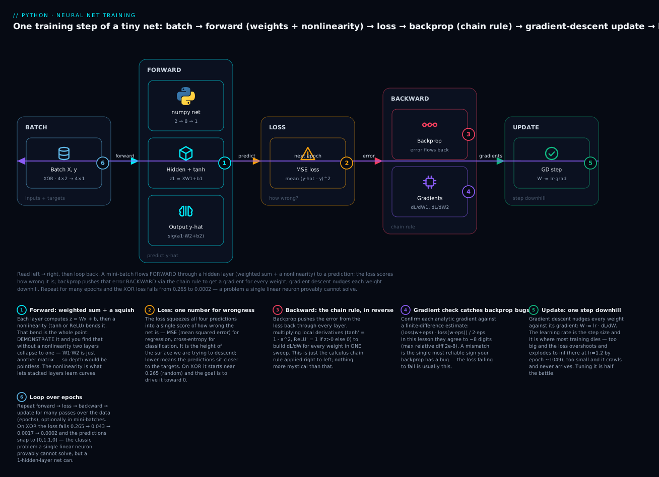
The diagram traces one full turn of that cycle and the ideas to carry out of this lesson: the forward pass is weighted sums plus the nonlinearity that stops depth collapsing (1); the loss squeezes wrongness into one number (2); backprop is the chain rule run right-to-left to get every gradient in one sweep (3); a finite-difference check is how you prove those gradients are right (4); the gradient-descent update is where the learning rate makes or breaks training (5); and you loop the whole thing over epochs until the loss bottoms out (6).
Now the centerpiece. XOR (exclusive-or) outputs 1 when its two binary inputs differ, 0 when they match. It is the textbook example of a problem that is not linearly separable — you cannot draw a single straight line that puts the two 1s on one side and the two 0s on the other. A linear model therefore provably cannot solve it. A network with one hidden layer can, because the hidden layer bends the space until the classes become separable.
| x₁ | x₂ | XOR (y) | Why |
|---|---|---|---|
| 0 | 0 | 0 | same → 0 |
| 0 | 1 | 1 | differ → 1 |
| 1 | 0 | 1 | differ → 1 |
| 1 | 1 | 0 | same → 0 |
Here is the complete network — forward, loss, backward, update — in pure numpy, trained on XOR. This is every piece from the sections above, assembled and looped. Building the net from a handful of small, single-purpose functions (forward, backward, train) is the composable-functions style from Functional Python: map, filter, reduce & closures applied to numerics:
import numpy as np

X = np.array([[0.,0.], [0.,1.], [1.,0.], [1.,1.]])   # XOR inputs
y = np.array([[0.],   [1.],    [1.],    [0.]])        # XOR targets

def sigmoid(z): return 1 / (1 + np.exp(-z))

def init_params(H=8, seed=1):
    r = np.random.default_rng(seed)
    return {"W1": r.normal(0, 1, (2, H)), "b1": np.zeros((1, H)),
            "W2": r.normal(0, 1, (H, 1)), "b2": np.zeros((1, 1))}

def forward(p, X):
    z1 = X @ p["W1"] + p["b1"];  a1 = np.tanh(z1)      # hidden: tanh
    z2 = a1 @ p["W2"] + p["b2"]; a2 = sigmoid(z2)      # output: sigmoid
    return {"z1": z1, "a1": a1, "z2": z2, "a2": a2}

def mse(a2, y): return float(np.mean((a2 - y) ** 2))

def backward(p, c, X, y):
    N = X.shape[0]
    dz2 = (2/N) * (c["a2"] - y) * c["a2"] * (1 - c["a2"])   # MSE' × sigmoid'
    dW2 = c["a1"].T @ dz2;  db2 = dz2.sum(0, keepdims=True)
    da1 = dz2 @ p["W2"].T
    dz1 = da1 * (1 - c["a1"]**2)                            # × tanh'
    dW1 = X.T @ dz1;  db1 = dz1.sum(0, keepdims=True)
    return {"W1": dW1, "b1": db1, "W2": dW2, "b2": db2}

def train(lr=0.5, epochs=5000, seed=1):
    p = init_params(seed=seed)
    history = []
    for e in range(epochs):
        c = forward(p, X)                    # 1. forward
        history.append(mse(c["a2"], y))      # 2. loss
        g = backward(p, c, X, y)             # 3. backward
        for k in p: p[k] -= lr * g[k]        # 4. update
    return p, history

params, history = train()
for e in (0, 200, 500, 1000, 2000, 4999):
    print(f"epoch {e:>4}: loss = {history[e]:.6f}")
preds = forward(params, X)["a2"]
print("final predictions:", preds.ravel().round(4))
print("rounded:", (preds.ravel() > 0.5).astype(int), " target:", y.ravel().astype(int))
epoch    0: loss = 0.264523
epoch  200: loss = 0.042999
epoch  500: loss = 0.006022
epoch 1000: loss = 0.001708
epoch 2000: loss = 0.000595
epoch 4999: loss = 0.000177
final predictions: [0.0093 0.9863 0.986  0.0154]
rounded: [0 1 1 0]  target: [0 1 1 0]
Watch what happened. The loss starts at 0.265 — the network outputs mush, roughly 0.5 everywhere. Within 200 epochs it has dropped to 0.043; by epoch 1000 it is 0.0017; it bottoms out near 0.0002. The final predictions are [0.009, 0.986, 0.986, 0.015] — hard against 0, 1, 1, 0. Rounded, they are exactly the XOR truth table. The network learned XOR by nothing but repeated forward/backward/update on four rows.
It is worth being concrete about how the hidden layer earns this, because it demystifies the whole “depth adds power” claim. Each hidden neuron computes w·x + b and fires (via tanh) on one side of a line in the 2-D input plane — a single neuron is exactly one dividing line, which is why one neuron alone can only ever cut the plane in two and cannot isolate XOR’s diagonal pair. But give the output neuron several such lines to combine, and it can carve out the region “input is on the high side of one line but the low side of another” — which is precisely the corner-shaped area XOR needs. The hidden layer’s job is to draw enough lines that the output neuron’s final weighted sum can separate the 1s from the 0s; gradient descent is what positions those lines. More hidden units means more lines to work with, which is the concrete meaning of “more capacity.”
Now the contrast that proves the hidden layer earned its place. Strip it out — a single sigmoid neuron, i.e. logistic regression, trained the same way — and XOR is impossible:
r = np.random.default_rng(0)
w = r.normal(0, 1, (2, 1)); b = np.zeros((1, 1))
for _ in range(20000):                         # 20k steps — way more than enough
    a = sigmoid(X @ w + b)
    dz = (2/4) * (a - y) * a * (1 - a)
    w -= 0.5 * (X.T @ dz);  b -= 0.5 * dz.sum(0, keepdims=True)

a = sigmoid(X @ w + b)
print("linear model preds:", a.ravel().round(4))   # => [0.5 0.5 0.5 0.5]
print("loss    :", round(mse(a, y), 4))             # => 0.25
print("accuracy:", ((a.ravel() > 0.5) == (y.ravel() > 0.5)).mean())  # => 0.5
The single neuron gives up and predicts 0.5 for all four inputs — a loss of 0.25, 50% accuracy, a coin flip. No amount of training helps, because no straight line separates XOR; the best a linear model can do is sit on the fence. This is the concrete payoff of the whole lesson: the nonlinearity and the hidden layer are not decoration — they are the difference between a solvable and an unsolvable problem. The learning rate confirms the earlier lesson too; train the working net at different rates and you see the same crawl/converge story:
| Learning rate | Final loss (5000 epochs) | Predictions | Verdict |
|---|---|---|---|
0.001 |
0.236459 | [1, 1, 1, 0] | crawls — never learns XOR in time |
0.01 |
0.124409 | [0, 1, 1, 0] | slow, only just correct |
0.1 |
0.001713 | [0, 1, 1, 0] | good |
0.5 |
0.000177 | [0, 1, 1, 0] | good (our default) |
2.0 |
0.000034 | [0, 1, 1, 0] | still fine here (small clean problem) |
Everything you set rather than learn is a hyperparameter, and these are the knobs you will spend real time tuning. Keep this glossary handy — most training problems trace back to one of these being wrong:
| Hyperparameter | Controls | Typical range | If wrong |
|---|---|---|---|
| Learning rate | step size of each update | 0.001–0.1 | too high → diverge; too low → crawl |
| Epochs | passes over the data | until the loss plateaus | too few → underfit; too many → overfit |
| Hidden units / layers | model capacity | problem-dependent | too few → underfit; too many → overfit |
| Batch size | samples per update | 32–512 | trades training speed against gradient noise |
| Init scale | starting spread of weights | small random | too big → explode; zero → symmetry trap |
What goes wrong (and how you know)
Neural networks fail in a small number of characteristic ways, and each has a fingerprint. Learn the fingerprints and debugging stops being guesswork.
Vanishing gradients. Backprop multiplies a local derivative at every layer. If those derivatives are consistently less than 1 — as sigmoid’s are, capping at 0.25 — the product shrinks geometrically, and by the time the error signal reaches the early layers it is effectively zero. Those layers stop learning. Watch a gradient signal decay through a stack of sigmoids:
r = np.random.default_rng(0)
for depth in (1, 3, 5, 10, 20):
    g = 1.0
    for _ in range(depth):
        v = sigmoid(r.normal())     # a typical activation
        g *= v * (1 - v)            # multiply by sigmoid' at each layer
    print(f"{depth:>2} sigmoid layers: gradient factor ~ {g:.3e}")
# =>  1 sigmoid layers: gradient factor ~ 2.490e-01
# =>  3 sigmoid layers: gradient factor ~ 1.403e-02
# =>  5 sigmoid layers: gradient factor ~ 4.220e-04
# => 10 sigmoid layers: gradient factor ~ 1.009e-07
# => 20 sigmoid layers: gradient factor ~ 1.138e-13
| Sigmoid layers deep | Gradient factor reaching layer 1 | Early-layer learning |
|---|---|---|
| 1 | 2.49×10⁻¹ | fine |
| 3 | 1.40×10⁻² | shrinking |
| 5 | 4.22×10⁻⁴ | weak |
| 10 | 1.01×10⁻⁷ | nearly frozen |
| 20 | 1.14×10⁻¹³ | dead |
Twenty sigmoid layers and the gradient reaching the first layer is ~10⁻¹³ — the early layers are frozen. This is the single biggest reason ReLU replaced sigmoid in hidden layers: ReLU’s derivative is exactly 1 for positive inputs, so it does not shrink the signal, and deep networks became trainable. Exploding gradients are the mirror image — derivatives consistently above 1 multiply up to huge values, nan out the weights, and are tamed by gradient clipping (cap the gradient’s magnitude) and careful initialization.
Weights initialized to zero — the symmetry trap. It is tempting to start all weights at 0. It is fatal. If every neuron in a layer starts identical, they receive identical gradients, update identically, and stay identical forever — the layer behaves like a single neuron no matter how wide it is. The network cannot break the symmetry, so it cannot learn. Set all our weights to zero and XOR is unreachable:
p = init_params(seed=1)
p["W1"][:] = 0.0;  p["W2"][:] = 0.0        # all weights zero
for _ in range(5000):
    c = forward(p, X); g = backward(p, c, X, y)
    for k in p: p[k] -= 0.5 * g[k]
print("final loss:", round(mse(forward(p, X)["a2"], y), 4))     # => 0.25
print("hidden columns all identical?", np.allclose(p["W1"], p["W1"][:, :1]))  # => True
print("predictions:", forward(p, X)["a2"].ravel().round(3))    # => [0.5 0.5 0.5 0.5]
Stuck at loss 0.25, every hidden neuron identical, predicting 0.5 — the same failure as having no hidden layer at all. This is why weights are initialized to small random values (and why schemes like Xavier/Glorot and He initialization, which scale that randomness to the layer size, matter for deep nets). Random init breaks the symmetry so neurons can specialize.
| Initialization | Effect | Verdict |
|---|---|---|
| All zeros / all equal | neurons stay identical — symmetry never breaks | broken — never use |
| Large random (e.g. ×10) | saturates activations, explodes gradients | unstable |
| Tiny random (e.g. ×0.001) | vanishing signal, painfully slow start | weak |
| Xavier/Glorot | variance scaled by fan-in + fan-out | good default for tanh/sigmoid |
| He | variance scaled by fan-in | good default for ReLU |
Unnormalized inputs. If one feature ranges 0–1 and another 0–100000, the weighted sum is dominated by the big one, gradients are lopsided, and training stalls or zig-zags. Neural networks want inputs on a common, modest scale — standardize features to roughly mean 0, standard deviation 1 (the StandardScaler idea from the ML fundamentals lesson) before training. The distribution-shaping intuition here is the descriptive-statistics material in Descriptive Statistics & Distributions; normalization is just recentering and rescaling each feature’s distribution.
Too little data. A network’s flexibility is a liability when data is scarce — it memorizes the handful of examples (overfits) and generalizes terribly. Neural nets are hungry; on a few hundred rows a linear model or a gradient-boosted tree usually wins. The generalization discipline from the ML fundamentals lesson — hold out a test set, watch the train-vs-test gap — is not optional here; it is life or death.
| Failure | Fingerprint | Cause | Fix |
|---|---|---|---|
| No nonlinearity | can’t learn XOR / any curve; acts linear | forgot the activation, or it’s linear | insert tanh/ReLU between layers |
| LR too high | loss rises, oscillates, or → inf/nan |
steps overshoot the minimum | lower LR 3–10×; clip gradients |
| LR too low | loss barely moves over many epochs | steps too small | raise LR 3–10× |
| Vanishing gradient | early layers don’t change; deep sigmoid net stalls | derivatives <1 multiply to ~0 | ReLU, residual connections, better init |
| Exploding gradient | weights → nan; loss spikes |
derivatives >1 multiply up | gradient clipping; smaller LR; better init |
| Dead ReLUs | many neurons always output 0; loss plateaus | pre-activation negative for all inputs | Leaky ReLU; lower LR; better init |
| Zero / equal init | loss stuck; all neurons identical | symmetry never breaks | small random init (Xavier/He) |
| Unnormalized inputs | slow, unstable training; one feature dominates | features on wildly different scales | standardize to mean 0, std 1 |
| Loss not falling | flat loss from step 1 | backprop bug (wrong gradient) | numerical gradient check |
| Great train, poor test | overfitting | too flexible for the data | more data; regularize; smaller net |
When a neural net beats classical ML — and when it loses
Neural networks are not a universal upgrade. They win decisively on unstructured data — inputs with rich internal structure that hand-engineered features can’t capture — and they lose, routinely, on the small tabular datasets that make up most business problems. Being honest about this saves you from the most common beginner mistake: reaching for a deep net where a boosted tree would have won with a tenth of the effort.
Where neural nets dominate is exactly where the input is high-dimensional and structured in a way a human can’t easily featurize: the pixels of an image, the waveform of audio, the token sequence of text, video, sensor streams. Here the network’s ability to learn its own features — edges then shapes then objects, in vision — beats anything you could code by hand, and nothing else is close. Convolutional networks own images; transformers own text and are how large language models work.
But for structured, tabular data — rows and columns of numbers and categories, the shape of most spreadsheets and databases — the honest, repeatedly-benchmarked verdict is that gradient-boosted trees (XGBoost, LightGBM, HistGradientBoosting) usually beat a neural network, and they train faster, need less tuning, need less data, and are easier to interpret. This ties straight back to the model-family map in ML Fundamentals: Supervised vs Unsupervised: match the model to the data shape, start with the simplest strong baseline, and only escalate to a neural net if it measurably wins on held-out data. On a 5,000-row tabular problem, that escalation rarely pays.
| Data type | Usual winner | Why |
|---|---|---|
| Images | CNN / vision transformer | learns spatial features (edges → objects) no one can hand-code |
| Text / language | transformer (LLMs) | learns meaning from token sequences at scale |
| Audio / speech | neural nets (CNN/RNN/transformer) | learns from raw waveform/spectrogram structure |
| Time series / sequences | neural nets, sometimes boosting | captures long-range temporal patterns |
| Tabular (rows × columns) | gradient-boosted trees | faster, needs less data/tuning, more interpretable |
| Small data (< ~1000s rows) | classical ML (linear, trees) | neural nets overfit; not enough to learn features |
| Need interpretability | linear / single tree | a neural net is opaque by default |
The rule of thumb: unstructured data and lots of it → neural network; structured tabular data → start with boosting. Deep learning is a spectacular tool aimed at a specific target, not a hammer for every nail.
Hands-on lab
Build the whole thing yourself, end to end, and reproduce every headline number. Everything is seeded, so your output will match the comments. One file, run with python nn_lab.py.
Setup (once):
python3 -m venv .venv && source .venv/bin/activate    # Windows: .venv\Scripts\activate
pip install numpy matplotlib
Step 1 — the network, forward and backward. Type this scaffold into nn_lab.py. It is the same net from the XOR section; the point is to build it with your own hands.
import numpy as np
X = np.array([[0.,0.],[0.,1.],[1.,0.],[1.,1.]])
y = np.array([[0.],  [1.],   [1.],   [0.]])

def sigmoid(z): return 1 / (1 + np.exp(-z))

def init_params(H=8, seed=1):
    r = np.random.default_rng(seed)
    return {"W1": r.normal(0,1,(2,H)), "b1": np.zeros((1,H)),
            "W2": r.normal(0,1,(H,1)), "b2": np.zeros((1,1))}

def forward(p, X):
    z1 = X @ p["W1"] + p["b1"]; a1 = np.tanh(z1)
    z2 = a1 @ p["W2"] + p["b2"]; a2 = sigmoid(z2)
    return {"z1":z1, "a1":a1, "z2":z2, "a2":a2}

def mse(a2, y): return float(np.mean((a2 - y)**2))

def backward(p, c, X, y):
    N = X.shape[0]
    dz2 = (2/N)*(c["a2"]-y)*c["a2"]*(1-c["a2"])
    dW2 = c["a1"].T @ dz2; db2 = dz2.sum(0, keepdims=True)
    da1 = dz2 @ p["W2"].T; dz1 = da1*(1-c["a1"]**2)
    dW1 = X.T @ dz1; db1 = dz1.sum(0, keepdims=True)
    return {"W1":dW1, "b1":db1, "W2":dW2, "b2":db2}
What just happened: you have a complete 2-layer net as four small functions — parameters, forward, loss, backward. No framework, no magic, just numpy arrays.
Step 2 — prove your backprop is correct (do this before training anything). A network that trains on a wrong gradient silently produces garbage; the numerical check is your insurance.
def gradient_check(seed=3, eps=1e-6):
    p = init_params(H=4, seed=seed)
    c = forward(p, X); g = backward(p, c, X, y)      # analytic gradients
    max_abs, max_rel, n = 0.0, 0.0, 0
    for k in ("W1","b1","W2","b2"):
        P, G = p[k], g[k]
        for idx in np.ndindex(P.shape):
            old = P[idx]
            P[idx] = old + eps; lp = mse(forward(p, X)["a2"], y)
            P[idx] = old - eps; lm = mse(forward(p, X)["a2"], y)
            P[idx] = old
            num = (lp - lm) / (2*eps)                # numerical gradient
            max_abs = max(max_abs, abs(num - G[idx]))
            if abs(G[idx]) > 1e-7:
                max_rel = max(max_rel, abs(num - G[idx]) / abs(G[idx])); n += 1
    print(f"max absolute diff: {max_abs:.2e}")
    print(f"max relative diff: {max_rel:.2e}  (over {n} params)")

gradient_check()
# => max absolute diff: 5.89e-11
# => max relative diff: 2.29e-08  (over 17 params)
What just happened: your hand-derived gradients match the finite-difference estimate to ~8 significant figures (relative diff 2e-8). That near-zero mismatch is your proof the backward pass is right. If you ever see a relative diff above ~1e-4, you have a bug in backward — hunt it before you train.
Step 3 — train on XOR and watch the loss fall.
def train(lr=0.5, epochs=5000, seed=1):
    p = init_params(seed=seed); history = []
    for e in range(epochs):
        c = forward(p, X); history.append(mse(c["a2"], y))
        g = backward(p, c, X, y)
        for k in p: p[k] -= lr * g[k]
    return p, history

params, history = train()
for e in (0, 200, 1000, 4999):
    print(f"epoch {e:>4}: loss = {history[e]:.6f}")
preds = forward(params, X)["a2"].ravel()
print("preds:", preds.round(3), "-> rounded:", (preds > 0.5).astype(int))
# => epoch    0: loss = 0.264523
# => epoch  200: loss = 0.042999
# => epoch 1000: loss = 0.001708
# => epoch 4999: loss = 0.000177
# => preds: [0.009 0.986 0.986 0.015] -> rounded: [0 1 1 0]
What just happened: the loss fell three-plus orders of magnitude and the predictions locked onto the XOR truth table [0,1,1,0]. You trained a neural network from scratch.
Step 4 — save the loss curve (headless).
import matplotlib
matplotlib.use("Agg")               # render without a display
import matplotlib.pyplot as plt

_, hist = train()
plt.figure(figsize=(7, 4))
plt.plot(hist)
plt.yscale("log")
plt.xlabel("epoch"); plt.ylabel("MSE loss (log)")
plt.title("XOR: loss falls from 0.265 to 0.0002")
plt.tight_layout(); plt.savefig("xor_loss.png", dpi=110)
print("saved -> xor_loss.png")
What just happened: xor_loss.png shows a clean downhill slide (log scale) — the visual signature of a network that is learning. A curve that is flat means a bug or a dead learning rate; a curve that rises means the learning rate is too high.
Step 5 — break it three ways, on purpose. Seeing the failures cements the fingerprints.
# (a) learning rate too high -> loss explodes/collapses
_, h_hi = train(lr=50.0)
print("lr=50  final loss:", round(h_hi[-1], 4))          # => 0.5  (collapsed, useless)

# (b) all-zero init -> symmetry never breaks
p = init_params(); p["W1"][:] = 0; p["W2"][:] = 0
for _ in range(5000):
    c = forward(p, X); g = backward(p, c, X, y)
    for k in p: p[k] -= 0.5 * g[k]
print("zero-init loss:", round(mse(forward(p, X)["a2"], y), 4))   # => 0.25 (stuck)

# (c) linear model (no hidden layer) cannot solve XOR
r = np.random.default_rng(0); w = r.normal(0,1,(2,1)); b = np.zeros((1,1))
for _ in range(20000):
    a = sigmoid(X @ w + b); dz = (2/4)*(a-y)*a*(1-a)
    w -= 0.5*(X.T@dz); b -= 0.5*dz.sum(0, keepdims=True)
print("linear XOR preds:", sigmoid(X @ w + b).ravel().round(2))   # => [0.5 0.5 0.5 0.5]
What just happened: a runaway learning rate collapses the net (loss 0.5), zero-init freezes it (loss 0.25), and a hidden-layer-free linear model flatlines at 0.5 everywhere — three of the most common ways real training dies, reproduced in a few lines. You now recognize all three on sight.
Common mistakes and troubleshooting
| Symptom / traceback | Cause | Fix |
|---|---|---|
| Loss flat from epoch 1, never moves | backprop bug — wrong gradient | run the numerical gradient check; fix backward until diff < 1e-4 |
Loss → inf or nan after a few epochs |
learning rate too high; exploding gradients | lower LR 3–10×; clip gradients; standardize inputs |
| Loss decreases painfully slowly | learning rate too low | raise LR 3–10× |
ValueError: matmul: ... mismatch |
wrong array shapes in a layer | check every W is (fan_in, fan_out); print .shape at each step |
| Network can’t learn XOR / any curve | no nonlinearity, or too few hidden units | add tanh/ReLU between layers; widen the hidden layer |
| All hidden neurons identical; loss stuck | weights initialized to zero (or all equal) | initialize to small random values (Xavier/He) |
| Deep net’s early layers never change | vanishing gradients (sigmoid/tanh depth) | use ReLU; add residual connections; better init |
| Many neurons permanently output 0 | dead ReLUs (all-negative pre-activation) | Leaky ReLU; lower LR; better init |
| Training unstable, one feature dominates | inputs not normalized | standardize features to mean 0, std 1 |
| Perfect on train, awful on new data | overfitting (net too flexible for the data) | more data; smaller net; regularization; early stopping |
RuntimeWarning: overflow in exp |
huge pre-activations into sigmoid/exp | lower LR; normalize inputs; clip logits |
| Great accuracy but a boosted tree beats it | used a NN on small tabular data | use gradient boosting; NNs shine on unstructured data |
The three that cost beginners the most time, in prose:
A loss that will not fall is almost always a backprop bug, and the gradient check finds it in two minutes. Beginners stare at the architecture, tweak the learning rate, add layers — when the real problem is a transposed matrix or a missing (1 − a²) in the backward pass, silently feeding gradient descent a wrong direction. Gradient descent then wanders or freezes. The discipline that saves hours: never trust a hand-written backward pass until the numerical gradient check passes. It needs no calculus — nudge a weight, remeasure the loss, compare — and it is definitive. A relative difference under 1e-6 means correct; above 1e-3 means bug.
nan in the loss is the learning rate shouting at you. When the loss becomes inf or nan, the overwhelmingly likely cause is a step size so large that a weight overshot into a region where the loss overflows floating point, and the poison spreads (any arithmetic with nan yields nan). The reflex is to divide the learning rate by 10 and rerun. If that alone fixes it, you were diverging; if it merely delays the nan, look next at unnormalized inputs feeding giant values into exp, or exploding gradients needing clipping. nan is never random — it is a number that grew too big, and something made it grow.
A neural network on small tabular data is usually the wrong tool, and the fix is to use a simpler model. The excitement of deep learning lures beginners into throwing a multi-layer net at a 2,000-row spreadsheet, where it overfits, needs babysitting, and loses to a gradient-boosted tree that trains in seconds. This is not a tuning problem you can fix with more epochs — it is a model-choice problem. Match the tool to the data: unstructured and abundant → neural net; structured, tabular, modest → boosting or a linear baseline first. The professional instinct from the ML fundamentals lesson holds — simplest strong baseline first, escalate only on measured, held-out wins.
Cheat-sheet
| Concept | Code / formula | Note |
|---|---|---|
| Neuron | a = activation(w @ x + b) |
weighted sum + bias, then a squish |
| Layer (batched) | A = activation(X @ W + b) |
W is (fan_in, fan_out) |
| Sigmoid / its derivative | 1/(1+np.exp(-z)) · a*(1-a) |
output layer; derivative maxes at 0.25 |
| Tanh / its derivative | np.tanh(z) · 1-a**2 |
zero-centered hidden activation |
| ReLU / its derivative | np.maximum(0,z) · (z>0) |
default deep hidden layer; watch dead neurons |
| Forward pass | z1=X@W1+b1; a1=f(z1); z2=a1@W2+b2; ... |
chain layers left → right |
| MSE loss | np.mean((y_hat - y)**2) |
regression |
| Binary cross-entropy | -mean(y*log(p)+(1-y)*log(1-p)) |
classification (probabilities) |
| Gradient descent step | W -= lr * dL_dW |
step against the gradient |
| Backprop rule | dL_dW = (layer input).T @ (error at layer) |
error flows right → left |
| tanh backprop | dz1 = da1 * (1 - a1**2) |
multiply by the activation’s derivative |
| Numerical gradient check | (loss(w+eps)-loss(w-eps))/(2*eps) |
must match analytic to ~1e-6 |
| Training loop | forward → loss → backward → update, repeat | one full pass = one epoch |
| Init weights | rng.normal(0, small, shape) |
random, never all-zero |
| Reproducibility | np.random.default_rng(seed) |
seed everything |
| LR too high / low | loss inf/nan / loss barely moves |
lower / raise 3–10× |
| Vanishing gradient | deep sigmoid/tanh; early layers freeze | switch to ReLU |
| NN vs boosting | unstructured → NN; tabular → boosting | match model to data shape |
Interview and exam questions
Q: In one honest sentence, what is a neural network?
A: A function built by chaining together weighted sums (W·x + b) each followed by a nonlinear activation, whose weights are tuned by gradient descent to minimize a loss on training data. It is loosely brain-inspired but is really just linear algebra plus a nonlinearity plus the calculus chain rule — no cognition, just a very flexible function with tunable knobs.
Q: Why do you need a nonlinear activation function? What happens without one?
A: Without a nonlinearity, stacking layers is pointless — a composition of linear maps is itself linear, so any number of linear layers collapses to a single equivalent linear layer (X W₁ W₂ = X W for W = W₁W₂). The whole network would have exactly the expressive power of one linear model. The nonlinearity between layers is what lets depth build up complex, curved functions; it is the one ingredient that makes “deep” meaningful.
Q: Compare sigmoid, tanh, and ReLU. Why did ReLU largely replace sigmoid in hidden layers?
A: Sigmoid squashes to (0,1) but its derivative caps at 0.25, so gradients shrink at every layer and vanish in deep nets; it is also not zero-centered. Tanh is zero-centered (−1,1) with derivative up to 1, better but still saturates. ReLU is max(0,z) — cheap (no exp), and its derivative is exactly 1 for positive inputs, so it does not shrink gradients, which made deep networks trainable. ReLU’s cost is “dead neurons”: a unit stuck with negative pre-activation for all inputs has zero gradient and never recovers (Leaky ReLU fixes this).
Q: What is a loss function, and which do you use for regression vs classification? A: A loss is a single number measuring how wrong the network’s predictions are; training minimizes it. For regression, use mean squared error (average squared error, punishes big misses quadratically). For classification, use cross-entropy on predicted probabilities, which punishes confident wrong answers harshly and trains faster than MSE on probabilities.
Q: Explain gradient descent and the role of the learning rate.
A: The loss is a surface over weight-space; the gradient points uphill, so you step the weights in the opposite (downhill) direction: W -= lr · ∂loss/∂W, repeated. The learning rate is the step size. Too small and training crawls (loss barely moves); too large and steps overshoot the minimum, oscillate, and can diverge to inf/nan. There is no universal value — you sweep a few (e.g. 0.001, 0.01, 0.1) and watch the loss curve.
Q: What is backpropagation, in plain terms?
A: It is the chain rule from calculus applied backward through the network to compute how much each weight contributed to the loss — i.e. ∂loss/∂W for every weight — in a single sweep that costs about one forward pass. Error flows right to left; at each layer the weight’s gradient is (that layer's input)ᵀ @ (the error arriving at that layer), and you multiply by the activation’s derivative to pass the error through it. Those gradients are exactly what gradient descent needs.
Q: How do you know your backprop implementation is correct?
A: Numerical gradient checking. For each weight, estimate the gradient by finite difference — (loss(w+ε) − loss(w−ε)) / 2ε for tiny ε — and compare to your analytic gradient. They should agree to roughly 1e-6 relative error; a larger mismatch means a bug in the backward pass. It is the single most valuable debugging tool, and it needs no calculus.
Q: Why can’t a single linear neuron (logistic regression) solve XOR, but a one-hidden-layer net can? A: XOR is not linearly separable — no single straight line puts both 1s on one side and both 0s on the other — so a linear model can only sit on the fence and predicts ~0.5 for all inputs (loss 0.25, 50% accuracy). A hidden layer with a nonlinearity warps the input space until the classes become linearly separable, so the output neuron can then split them. XOR is the classic proof that depth + nonlinearity add real power.
Q: What are vanishing and exploding gradients, and how do you address them?
A: Backprop multiplies a local derivative at each layer. If those are consistently below 1 (sigmoid’s cap 0.25), the product shrinks geometrically and early-layer gradients vanish toward zero — those layers stop learning (fix: ReLU, residual connections, better init). If consistently above 1, gradients explode to huge values and nan the weights (fix: gradient clipping, smaller learning rate, careful initialization).
Q: Why must weights be initialized to small random values rather than zero? A: If all weights start equal (e.g. zero), every neuron in a layer computes the same output, receives the same gradient, and updates identically — so they stay identical forever and the layer acts like a single neuron. Symmetry is never broken and the network can’t learn (on XOR it stays stuck at loss 0.25). Small random init breaks the symmetry so neurons specialize; Xavier/He schemes scale that randomness to the layer size for stable deep training.
Q: When should you reach for a neural network, and when is it the wrong tool? A: Use neural nets for unstructured data with lots of it — images, audio, text, sequences — where they learn features no one could hand-code (CNNs for vision, transformers for language). Avoid them for small structured/tabular data, where gradient-boosted trees (XGBoost, LightGBM) usually beat them while training faster, needing less data and tuning, and being more interpretable. Match the model to the data shape; start with the simplest strong baseline and escalate only on measured held-out wins.
Q (coding): Write the forward pass of a 2-layer net (tanh hidden, sigmoid output) in numpy. A:
def forward(X, W1, b1, W2, b2):
    z1 = X @ W1 + b1        # (N, H)  weighted sums for the hidden layer
    a1 = np.tanh(z1)        # (N, H)  hidden activations (nonlinearity!)
    z2 = a1 @ W2 + b2       # (N, 1)  output pre-activation
    return 1 / (1 + np.exp(-z2))   # (N, 1)  sigmoid predictions
The keys are the shapes (W is (fan_in, fan_out), output is one row per sample) and the nonlinearity between the layers — without np.tanh, this collapses to linear regression.
Key takeaways
- A neural network is chained linear algebra + a nonlinearity + calculus — a neuron is
activation(w·x + b), a layer is that batched with a matrix multiply, and “deep” just means more than one hidden layer. The brain analogy is marketing; the arithmetic is the truth, and you can write all of it in numpy. - The nonlinear activation is non-negotiable. Stacked linear layers collapse to a single linear layer (verified to machine precision), so without a nonlinearity depth buys nothing. Sigmoid and tanh saturate and vanish gradients; ReLU (
max(0,z)) won hidden layers by being cheap and not shrinking gradients — at the cost of dead neurons. - Training is minimizing a loss by gradient descent:
W -= lr · ∂loss/∂W, repeated. The learning rate is the make-or-break knob — too high and the loss explodes toinf, too low and it crawls — and there is no universal value, so you sweep and watch the curve. - Backpropagation is the chain rule applied backward to get every weight’s gradient in one sweep — nothing more mystical. Always confirm it with a numerical gradient check (
(loss(w+ε)−loss(w−ε))/2ε); a flat loss is almost always a backprop bug this check would catch. - The training loop is four steps — forward → loss → backward → update — repeated over epochs. On XOR, a problem a linear model provably cannot solve, a tiny 2-layer net drives the loss from 0.265 to 0.0002 and nails
[0,1,1,0], while the linear model flatlines at 0.5. - Know the failure fingerprints:
nanloss → LR too high; flat loss → backprop bug; frozen early layers → vanishing gradients (use ReLU); identical stuck neurons → zero init (use random); unstable training → normalize inputs. Each has a specific, learnable fix. - Neural nets win on unstructured data (images, text, audio) and lots of it; on small tabular data, gradient-boosted trees usually beat them. Match the model to the data shape, start simple, and escalate only when a held-out score earns it.