In the previous lesson you did something most people who use deep learning have never done: you built a neural network from nothing but NumPy arrays. You wrote the forward pass, and then — the hard part — you wrote the backward pass by hand, deriving ∂loss/∂w with the chain rule, one layer at a time, and updating the weights yourself. It worked. It also took a page of careful calculus that would become unmaintainable the moment the network grew past two layers or you swapped the loss function.
That hand-written backprop is the exact thing a deep learning framework exists to delete. This lesson takes the same job — classify data by training a small network — and hands it to PyTorch, the framework that runs most of modern AI research and a large share of production. You will see that PyTorch does not do anything magic: it does the specific, tedious, error-prone thing you just did by hand — computing gradients — automatically, correctly, for any network you can dream up, on a GPU if you have one. Everything else it gives you (prebuilt layers, optimizers, data loaders) is convenience on top of that one superpower.
Everything below was executed on CPython 3.12.3 with PyTorch 2.13.0, scikit-learn 1.9.0, and NumPy 2.5.1; the Keras half ran on TensorFlow 2.21.0 / Keras 3.15.0. Every loss curve, accuracy number, and traceback on this page is copied from a real run — including the deliberately broken one where the loss climbs to 3.4 million. If you run the code, you will get these numbers (or numbers a hair away, since some randomness survives even a fixed seed).
Why this matters: what a framework actually automates
Here is the mental model that makes PyTorch click. Your hand-built net had three moving parts: a forward pass (turn inputs into a prediction), a loss (score how wrong the prediction is), and a backward pass (compute how to nudge every weight to make the loss smaller). The forward pass and the loss are easy — they are just arithmetic you write once. The backward pass is where people drown: every new layer, activation, or loss means re-deriving gradients, and one sign error silently ruins training with no traceback to tell you.
A framework’s headline feature is automatic differentiation (autograd): you write only the forward pass, and the framework watches every operation you perform, builds a graph of them, and can then compute the exact gradient of the output with respect to every input — automatically, by mechanically applying the chain rule you applied by hand. You get correct backprop for free, for arbitrary networks. That single feature is why frameworks won.
Autograd is the reason to switch, but not the only thing you get. Four more come in the box:
| What you did by hand in NumPy | What the framework gives you | Why it matters |
|---|---|---|
Derived ∂loss/∂w with the chain rule |
Autograd — loss.backward() fills every gradient |
No manual calculus; correct for any network |
Ran on CPU, one core, float64 |
GPU/accelerator — .to("cuda")/"mps" |
10–100× faster training on real data |
Wrote w @ x + b, ReLU, softmax yourself |
Prebuilt layers — nn.Linear, nn.ReLU, … |
Tested, fast, composable building blocks |
Coded the weight update w -= lr * grad |
Optimizers — SGD, Adam, AdamW |
Adaptive learning rates, momentum, decay — one line |
| Wrote your own MSE / cross-entropy | Losses — CrossEntropyLoss, MSELoss |
Numerically stable, edge-cases handled |
It is worth being precise about which line of your hand-built net disappears, because that is the whole pitch. Your NumPy net had a forward pass — matrix multiplies, a ReLU, a softmax — and you kept every one of those. What you delete is the mirror-image block underneath it: the manual d_loss, d_w2, d_b2, d_hidden, d_w1 derivations, each a hand-applied chain-rule step that had to be re-derived the instant you changed a layer or a loss. In PyTorch that entire block becomes the single call loss.backward(). You describe only the forward computation — the thing you actually understand — and the gradients come for free, correct, for any architecture. That is not a convenience; it is the difference between networks you can hand-differentiate (two or three layers) and the ones that run the world (dozens to hundreds).
The second reason is scale through hardware. Your NumPy net ran on the CPU in float64, one operation at a time. A framework tensor moves to a GPU with .to("cuda") and the same matrix multiplies run across thousands of GPU cores in float32, the format the hardware is built for — routinely 10–100× faster on real networks, which is the difference between an experiment that takes an hour and one that takes a week. We force CPU in this lesson because the model is tiny and reproducibility matters more than speed, but the code is GPU-ready by design: write it once, move a device, and it scales.
There is also the ecosystem, which is half the reason a framework is worth learning: pretrained models, datasets, tutorials, and higher-level libraries (PyTorch Lightning, Hugging Face, fastai) all assume you speak PyTorch or Keras. Learn the framework and the entire modern-AI toolbox opens; stay in hand-rolled NumPy and you are alone.
One honest caveat before you fall in love, in the spirit of the ML fundamentals lesson’s “when not to use ML”: a neural network is not the default answer to a prediction problem. On small-to-medium tabular data — the spreadsheets most businesses actually have — a gradient-boosted tree (XGBoost, LightGBM) or even a plain scikit-learn RandomForest usually matches or beats a neural net, trains in seconds instead of minutes, needs no GPU, and requires almost no tuning. Deep learning earns its complexity on unstructured, high-dimensional data where features must be learned rather than engineered — images, audio, text, and other signals with spatial or sequential structure. Reach for PyTorch when the problem is genuinely that shape (or when you are learning, as here); reach for a tree when someone hands you a CSV of 5,000 rows and 20 columns. Using the biggest hammer in the shed on every nail is the most common beginner mistake in applied ML.
This lesson assumes you are comfortable with the ideas underneath: that a model learns a function from data (ML Fundamentals), that a fair score comes only from held-out data (Train/Test Splits & Metrics), and that everything numeric is a NumPy array under the hood. If fit/predict on a scikit-learn estimator is already reflex, you are perfectly placed — a framework is what you reach for when fit/predict is not flexible enough and you need to define the model yourself.
Set up a virtual environment — never install these heavy packages into the system Python:
python3 -m venv .venv
source .venv/bin/activate                 # Windows: .venv\Scripts\activate
python -m pip install --upgrade pip

# scikit-learn ships the digits dataset (no download) + preprocessing
pip install scikit-learn numpy

# PyTorch CPU-only build (~150 MB; the GPU builds are much larger).
# The CPU wheel runs everywhere and is all you need for this lesson.
pip install torch --index-url https://download.pytorch.org/whl/cpu

# Optional: the Keras half at the end needs TensorFlow
pip install tensorflow

python -c "import torch; print('torch', torch.__version__)"
# => torch 2.13.0
⚠️ The full CUDA PyTorch build is several gigabytes and only helps if you own an NVIDIA GPU. For learning — and for the tiny model in this lesson — the CPU wheel above is the right choice and trains in seconds. On Apple Silicon the standard wheel also gives you the mps accelerator for free.
Tensors: NumPy arrays that carry a gradient and a device
The atom of PyTorch is the tensor. If you know NumPy’s ndarray, you already know 90% of it: a tensor is an n-dimensional array of numbers of one dtype, with a shape and strides, supporting the same broadcasting and indexing. The 10% that is new — and the entire reason tensors exist rather than reusing NumPy — is two extra powers bolted onto that array:
- A tensor can track gradients (
requires_grad=True), so autograd can differentiate through it. - A tensor lives on a device (
cpu,cuda,mps), so the same code runs on a GPU by moving the data.
NumPy ndarray |
PyTorch Tensor |
|
|---|---|---|
| n-D array, one dtype, broadcasting | Yes | Yes (nearly identical API) |
| Default float dtype | float64 |
float32 (what GPUs like) |
| Runs on GPU | No | Yes — .to("cuda") / "mps" |
| Tracks gradients for autograd | No | Yes — requires_grad=True |
| Element-wise add | a + b |
a + b |
| Matrix multiply | a @ b |
a @ b |
| Reshape / transpose | .reshape / .T |
.reshape / .T (same) |
| Convert to the other | — | .numpy() ⇄ torch.from_numpy() |
import torch
import numpy as np

t = torch.tensor([[1.0, 2.0],
                  [3.0, 4.0]])
print(t)
# tensor([[1., 2.],
#         [3., 4.]])
print(t.shape, t.dtype, t.device)   # torch.Size([2, 2]) torch.float32 cpu
Two dtype facts bite beginners immediately. First, PyTorch defaults to float32, not NumPy’s float64 — GPUs are built for 32-bit floats, and using 64-bit doubles your memory for no accuracy the model needs. Second, integer labels for classification must be int64 (called long), because the loss function indexes into a probability table with them. Get a dtype wrong and you meet a RuntimeError (we trigger the real ones later).
The NumPy ⇄ tensor bridge (and the shared-memory trap)
You constantly cross between NumPy (for loading, sklearn, plotting) and tensors (for the model). Two functions do it, and there is one sharp edge: torch.from_numpy and .numpy() share the same memory buffer — they do not copy. Mutating one mutates the other.
a = np.array([1.0, 2.0, 3.0])
tb = torch.from_numpy(a)     # tensor VIEWS the same buffer as `a`
print(tb)                    # tensor([1., 2., 3.], dtype=torch.float64)

a[0] = 99.0                  # mutate the NumPy array...
print(tb)                    # ...and the tensor sees it:
                             # tensor([99.,  2.,  3.], dtype=torch.float64)

back = tb.numpy()            # back to NumPy — also a shared view
print(type(back))            # <class 'numpy.ndarray'>
| Task | Call | Copies? | Note |
|---|---|---|---|
| NumPy → tensor | torch.from_numpy(a) |
No — shared buffer | Keeps a’s dtype (often float64) |
| NumPy → tensor (fresh) | torch.tensor(a) |
Yes — safe copy | Use when you don’t want aliasing |
| Tensor → NumPy | t.numpy() |
No — shared buffer | Fails if t requires grad (see autograd) |
| Tensor → NumPy (safe) | t.detach().cpu().numpy() |
Yes | The idiom for grabbing model outputs |
| Set dtype on the way in | torch.tensor(a, dtype=torch.float32) |
Yes | The usual fix for the float64 surprise |
Notice from_numpy preserved float64. When you feed data to a model you almost always want torch.tensor(a, dtype=torch.float32) — building a fresh float32 copy in one step and dodging both the dtype mismatch and the aliasing surprise.
Tensor operations you will use constantly
Beyond arithmetic, a handful of shape-and-reduce operations show up in every model. They mirror NumPy, with one PyTorch-specific pair — view and reshape — worth distinguishing.
t = torch.arange(6.)                 # tensor([0., 1., 2., 3., 4., 5.])
print(t.reshape(2, 3))               # [[0,1,2],[3,4,5]]
print(t.view(3, 2))                  # same data, shape (3,2)  — view needs contiguous memory
print(t.unsqueeze(0).shape)          # torch.Size([1, 6])  — add a batch axis
print(torch.zeros(1, 6).squeeze().shape)  # torch.Size([6]) — drop size-1 axes

a = torch.tensor([[1., 2.], [3., 4.]])
print(a.mean().item(), a.mean(dim=0).tolist(), a.sum(dim=1).tolist())
# 2.5 [2.0, 3.0] [3.0, 7.0]
print(a.argmax(dim=1).tolist())      # [1, 1] — index of the max per row
| Operation | Call | Result / use |
|---|---|---|
| Reshape | t.reshape(2, 3) |
New shape, copies if needed |
| Reshape (no copy) | t.view(3, 2) |
Same buffer; requires contiguous memory |
| Add an axis | t.unsqueeze(0) |
(6,) → (1, 6) — make a single row a “batch of 1” |
| Drop size-1 axes | t.squeeze() |
(1, 6) → (6,) |
| Reduce all | t.mean(), t.sum() |
Scalar |
| Reduce one axis | t.mean(dim=0) |
Collapse rows → per-column mean |
| Concatenate | torch.cat([a, b], dim=0) |
Join along an existing axis |
| Stack | torch.stack([a, b]) |
Join along a new axis |
| Top class | logits.argmax(dim=1) |
Index of the max per row — this is prediction |
unsqueeze(0) earns special mention: models expect a batch dimension, so a single 64-pixel image (shape (64,)) must become (1, 64) before you can pass it to the model. Forgetting the batch axis is a frequent shape error at inference time.
Autograd: the framework does your backprop for you
This is the heart of the lesson, so we prove it rather than assert it. In the previous lesson you differentiated a loss by hand. Here PyTorch does the identical derivation automatically, and we check that the number it produces equals the one you would compute by hand.
Set requires_grad=True on a tensor and PyTorch starts recording every operation you perform on it into a dynamic computational graph — a record of “this tensor came from multiplying those two.” Call .backward() on the final scalar and autograd walks that graph in reverse, applying the chain rule, depositing ∂output/∂x into each input’s .grad.
Start with the simplest possible check: the derivative of f(x) = x² is 2x, which is 6 at x = 3.
import torch

x = torch.tensor(3.0, requires_grad=True)   # "track gradients for x"
f = x ** 2                                    # graph: f = x*x
f.backward()                                  # autograd walks it backward
print(x.grad)      # tensor(6.)   <- exactly 2*x at x=3. No calculus written.
Now the version that matters — a single linear neuron with a squared-error loss, the exact shape of the backprop you hand-derived. With weight w, bias b, input x, target t:
- prediction
p = w·x + b - loss
L = (p − t)² - by hand:
∂L/∂w = 2(p − t)·xand∂L/∂b = 2(p − t)
w = torch.tensor(2.0, requires_grad=True)
b = torch.tensor(0.5, requires_grad=True)
x = torch.tensor(1.5)
target = torch.tensor(5.0)

pred = w * x + b            # 2*1.5 + 0.5 = 3.5
loss = (pred - target) ** 2 # (3.5 - 5.0)**2 = 2.25
loss.backward()             # fill w.grad and b.grad automatically

print(pred.item(), loss.item())   # 3.5 2.25
print(w.grad.item())              # -4.5   hand: 2*(3.5-5)*1.5 = -4.5  ✔
print(b.grad.item())              # -3.0   hand: 2*(3.5-5)     = -3.0  ✔
The gradients autograd computed (-4.5, -3.0) are identical to the hand-derived formulas. That is the whole promise made concrete: you wrote the forward pass (w * x + b and the squared error) and nothing else; PyTorch produced the exact gradients that, last lesson, cost you a page of chain-rule algebra. Scale this from one neuron to a million and the value is obvious — you could never hand-derive backprop for a real network, and you never have to.
You can even see the graph autograd built. Chain two operations — y = 3x, then z = y², so z = 9x² and dz/dx = 18x — and each intermediate tensor carries a grad_fn recording the operation that made it:
x = torch.tensor(2.0, requires_grad=True)
y = 3 * x                 # y.grad_fn -> <MulBackward0>
z = y ** 2                # z.grad_fn -> <PowBackward0>
print(z.grad_fn)          # <PowBackward0 object at 0x...>
z.backward()
print(x.grad.item())      # 36.0   <- 18 * x at x=2, via the chain rule
Autograd walked z → y → x backward, multiplying local derivatives (dz/dy = 2y = 12, then dy/dx = 3) to get 12 × 3 = 36 — exactly the chain rule, executed for you. That linked list of grad_fns is the computational graph, and it is rebuilt from scratch on every forward pass, which is why ordinary Python control flow inside a model just works.
| Concept | What it is | Call / attribute |
|---|---|---|
| Track a tensor | Ask autograd to record ops on it | requires_grad=True |
| The graph | Dynamic record of operations, rebuilt every forward pass | (implicit) .grad_fn |
| Backprop | Walk the graph in reverse, apply chain rule | loss.backward() |
| The result | Gradient of the loss w.r.t. each parameter | param.grad |
| Turn it off | Stop recording (inference, no training) | with torch.no_grad(): |
| Snapshot without grad | Detach a tensor from the graph | t.detach() |
| Gradients accumulate | Each .backward() adds into .grad |
(this is the famous bug) |
Two details you must internalize. First, the graph is dynamic — it is built fresh on every forward pass, so you can use normal Python if/for/while inside a model and the graph simply reflects whatever ran. (This is PyTorch’s “define-by-run” model, and the reason it feels like ordinary Python.) Second — burn this in — .backward() adds to .grad, it does not overwrite it. Call backward twice without clearing, and the second gradient piles on top of the first. That accumulation is occasionally useful, but forgetting to clear it is the single most common bug in all of PyTorch, and we will detonate it on purpose later.
For pure inference you do not want the graph at all — building it wastes memory and time when you will never call .backward(). Wrap inference in torch.no_grad():
with torch.no_grad():
    y = w * x + b
print(y.requires_grad)   # False  — no graph built, faster + leaner
This is not a micro-optimization. To be able to run backward(), the graph must keep every intermediate value from the forward pass in memory (it needs them to compute the local derivatives). On a large model over a large batch, those stored activations are often the biggest single consumer of GPU memory — and at inference you will never call backward(), so keeping them is pure waste. torch.no_grad() tells PyTorch “don’t record, don’t retain,” which is why every correct inference and evaluation path in this lesson is wrapped in it. During training you do need the graph, which is the honest reason training a given model needs far more memory than serving it.
Building a model: nn.Module
You could keep individual w and b tensors and wire them by hand, but real models have thousands of parameters across many layers. PyTorch packages a model as a subclass of nn.Module: you declare the layers in __init__, and you describe how data flows through them in forward. The base class then tracks every parameter for you (so the optimizer can find them), handles moving the whole model to a device, and toggles train/eval mode.
The layers themselves are also nn.Modules. The three you need for a basic classifier:
| Layer | What it does | Key arguments |
|---|---|---|
nn.Linear(in, out) |
Fully-connected layer: x @ Wᵀ + b |
in_features, out_features |
nn.ReLU() |
Activation: max(0, x), adds non-linearity |
(none) |
nn.Dropout(p) |
Randomly zeroes a fraction p of activations in training only |
p (drop probability) |
nn.Sequential(...) |
Chains modules; its forward runs them in order |
the layers, in order |
nn.Flatten() |
Collapses trailing dims (e.g. image → vector) | (none) |
Here is a small multilayer perceptron (MLP) for the 8×8 digit images we will classify: 64 input pixels → a hidden layer of 32 with ReLU → dropout → 10 output scores (one per digit).
import torch.nn as nn

class DigitMLP(nn.Module):
    def __init__(self, in_features=64, hidden=32, classes=10, p_drop=0.2):
        super().__init__()                      # ALWAYS call this first
        self.net = nn.Sequential(
            nn.Linear(in_features, hidden),     # 64 -> 32
            nn.ReLU(),
            nn.Dropout(p_drop),                 # regularization
            nn.Linear(hidden, classes),         # 32 -> 10  (raw scores)
        )

    def forward(self, x):
        return self.net(x)                      # define-by-run: just call it

model = DigitMLP()
print(model)
# DigitMLP(
#   (net): Sequential(
#     (0): Linear(in_features=64, out_features=32, bias=True)
#     (1): ReLU()
#     (2): Dropout(p=0.2, inplace=False)
#     (3): Linear(in_features=32, out_features=10, bias=True)
#   )
# )
print(sum(p.numel() for p in model.parameters()))   # 2410 trainable params
Three rules that save hours. One: call super().__init__() as the first line of your __init__, or PyTorch cannot register your parameters and the optimizer will silently train nothing. Two: the last layer outputs raw scores called logits — do not put a softmax there. The standard classification loss expects logits and applies softmax internally, in a numerically stable way (adding your own softmax makes the loss wrong, as we will demonstrate). Three: you never call model.forward(x) directly — you call model(x), which runs forward plus the framework’s bookkeeping (hooks, train/eval state). The 2,410 parameters are 64×32 + 32 (first layer) + 32×10 + 10 (second) — every one of which autograd will differentiate for you.
The nn.ReLU() between the two linear layers is the activation function, and it is not optional: two linear layers with nothing between them collapse mathematically into a single linear layer, so the network could only ever learn straight-line relationships. A non-linear activation is what lets a network bend to fit complex patterns. ReLU (max(0, x)) is the default because it is cheap and trains well; the others have their niches.
| Activation | Formula | Range | Use for | x=[-2, 0, 1, 3] → |
|---|---|---|---|---|
| ReLU | max(0, x) |
[0, ∞) |
Hidden layers (default) | [0, 0, 1, 3] |
| Sigmoid | 1/(1+e⁻ˣ) |
(0, 1) |
Binary output probability | [0.12, 0.5, 0.73, 0.95] |
| Tanh | tanh(x) |
(−1, 1) |
Older hidden layers, RNNs | [−0.96, 0, 0.76, 0.995] |
| Softmax | eˣⁱ/Σeˣ |
sums to 1 | Multi-class output (probabilities) | [0.006, 0.041, 0.111, 0.818] |
| GELU | smooth ReLU | ≈[0, ∞) |
Transformers | — |
You can inspect exactly what the base class registered. model.parameters() is what you hand the optimizer; named_parameters() shows you the tree, and state_dict() is what you save:
for name, p in model.named_parameters():
    print(name, tuple(p.shape), p.requires_grad)
# net.0.weight (32, 64) True     net.0.bias (32,) True
# net.3.weight (10, 32) True     net.3.bias (10,) True
| Accessor | Returns | Used for |
|---|---|---|
model.parameters() |
Iterator of weight tensors | Handed to the optimizer |
model.named_parameters() |
(name, tensor) pairs |
Inspection, freezing specific layers |
model.state_dict() |
OrderedDict of all weights |
Saving / loading |
p.numel() |
Element count of a tensor | Counting total parameters |
p.requires_grad = False |
Freeze a parameter | Transfer learning / fine-tuning |
Feeding data: Dataset and DataLoader
You almost never train on the whole dataset at once — you train on mini-batches (say 64 rows at a time), because batches fit in memory, give a smoother gradient than one row, and let the GPU parallelize. PyTorch splits this into two objects: a Dataset knows how to fetch one example (dataset[i] → (features, label)), and a DataLoader wraps a dataset to yield shuffled batches.
For in-memory arrays, TensorDataset is the shortcut — hand it feature and label tensors and it pairs them up:
from torch.utils.data import TensorDataset, DataLoader

# Xtr, ytr are tensors: features float32, labels int64 (long)
train_ds = TensorDataset(Xtr, ytr)
train_dl = DataLoader(train_ds, batch_size=64, shuffle=True)

print(len(train_dl))                 # 23   (1437 rows / 64 ≈ 23 batches)
xb, yb = next(iter(train_dl))
print(xb.shape, yb.shape)            # torch.Size([64, 64]) torch.Size([64])
DataLoader argument |
What it controls | Typical value |
|---|---|---|
batch_size |
Rows per batch | 32 / 64 / 128 |
shuffle |
Reshuffle every epoch (train only!) | True for train, False for val/test |
num_workers |
Background loading processes | 0 on CPU/small, 2–8 for big data |
drop_last |
Drop the final undersized batch | False usually |
pin_memory |
Faster CPU→GPU transfer | True when training on CUDA |
shuffle=True matters more than it looks: if your data is sorted by label, un-shuffled batches show the model all the 0s, then all the 1s, and each batch’s gradient yanks the weights toward whichever class it contains. Shuffle for training, never for validation or test (there is no gradient there, and you want reproducible evaluation).
Batch size is a real knob, not a formality: it sets how many batches (and therefore how many weight updates) you get per epoch. Our 1,437 training rows split like this:
batch_size |
Batches / epoch | Trade-off |
|---|---|---|
| 32 | 45 | More updates/epoch, noisier gradients — often generalizes well |
| 64 | 23 | The common default; a good balance |
| 128 | 12 | Smoother gradient, fewer updates, more memory |
| 256 | 6 | Fast per epoch but may need more epochs / higher LR |
Smaller batches give noisier but more frequent gradient steps (the noise can even help escape bad minima); larger batches give a smoother gradient and use the hardware better but need more memory and sometimes a higher learning rate to converge in the same number of epochs. When in doubt, 32 or 64.
The canonical training loop
Everything so far converges here. The PyTorch training loop is five lines that every practitioner memorizes, run once per batch, wrapped in a loop over epochs. Learn these five and their order and you can train any PyTorch model on earth.
for epoch in range(EPOCHS):
    model.train()                        # training mode (dropout ON)
    for xb, yb in train_dl:              # one mini-batch
        optimizer.zero_grad()            # 1. clear last batch's gradients
        pred = model(xb)                 # 2. forward pass (builds the graph)
        loss = criterion(pred, yb)       # 3. how wrong are we?
        loss.backward()                  # 4. autograd fills every .grad
        optimizer.step()                 # 5. optimizer nudges the weights
Read them as a sentence: clear the old gradients, predict, score, back-propagate, step. The diagram below traces one trip through the loop and marks the exact point the classic bug bites.
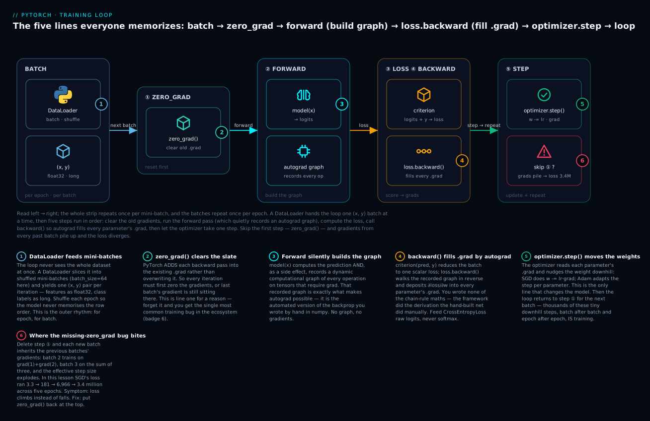
Underneath those five lines is one idea: gradient descent. The loss is a landscape over the millions of weight values, and the gradient param.grad points in the direction of steepest increase of the loss. So to reduce the loss you step the opposite way — w = w - lr * grad — a little downhill, over and over. backward() computes which way is downhill for every weight at once; step() takes the step; the learning rate lr sets how big. Run that a few thousand times over shuffled batches and the weights settle into a valley where the loss is low — which is to say, the model has learned. Every framework, every optimizer, every architecture is a variation on this single loop; internalize it and deep learning stops being mysterious.
The one line beginners drop is optimizer.zero_grad(), and dropping it is catastrophic precisely because — as you saw with autograd — .backward() adds to .grad. Without the clear, batch 2 trains on grad(batch1) + grad(batch2), batch 3 on the sum of three, and the effective step size explodes. We will watch that happen for real in the lab.
| Line | Call | What happens | Skip it and… |
|---|---|---|---|
| 1 | optimizer.zero_grad() |
Reset every .grad to zero |
Gradients accumulate → loss diverges |
| 2 | pred = model(x) |
Forward pass; records the autograd graph | Nothing to differentiate |
| 3 | loss = criterion(pred, y) |
Reduce the batch to one scalar loss | No signal to minimize |
| 4 | loss.backward() |
Autograd fills param.grad for all params |
.grad stays None; step does nothing |
| 5 | optimizer.step() |
Update weights using .grad |
Weights never change; no learning |
Losses and optimizers
The loss (criterion) measures wrongness; the optimizer decides how to move the weights to reduce it. You pick one of each off the shelf.
| Loss | Use for | Feed it | Gotcha |
|---|---|---|---|
nn.CrossEntropyLoss |
Multi-class classification | logits + integer class indices (long) |
Applies softmax internally — never pre-softmax |
nn.BCEWithLogitsLoss |
Binary / multi-label | logits + float 0/1 targets | Also stable; don’t add sigmoid yourself |
nn.MSELoss |
Regression | prediction + float target | Same shape both sides |
nn.L1Loss |
Regression, robust to outliers | prediction + float target | Mean absolute error |
Why these pairings? Classification asks “which of these classes,” and cross-entropy measures how much probability mass the model put on the right class — punishing confident wrong answers far more than hesitant ones, which is exactly the pressure you want. Regression asks “what number,” and MSE measures squared distance from the true value — punishing big misses quadratically. Matching the loss to the question is not a formality; a regression loss on a classification problem gives the optimizer the wrong thing to minimize.
CrossEntropyLoss deserves the emphasis it gets: it wants raw logits and integer class labels, and it fuses LogSoftmax + NLLLoss for numerical stability. Two mistakes flow from misunderstanding this — feeding it your own softmax output (it silently double-counts and gives a wrong number), or feeding float/one-hot labels where it wants integer indices (a RuntimeError). Both appear in the troubleshooting table with their real messages.
| Optimizer | Idea | When to reach for it |
|---|---|---|
torch.optim.SGD |
w -= lr * grad (+ optional momentum) |
Simple, well-understood; strong with a tuned LR + momentum |
torch.optim.Adam |
Per-parameter adaptive learning rate | The reliable default — works out of the box |
torch.optim.AdamW |
Adam with correct weight decay | Modern default for transformers / big nets |
torch.optim.RMSprop |
Adaptive, older | Occasionally in RL / RNNs |
SGD vs Adam in one breath: SGD applies the raw gradient scaled by one global learning rate, so it is sensitive to that LR but converges to clean solutions; Adam keeps a per-parameter running estimate of the gradient’s size and normalizes by it, so it trains fast and forgives a badly-chosen LR. Start with Adam(model.parameters(), lr=1e-3) — it is the “just works” choice — and only reach for tuned SGD when you are chasing the last fraction of accuracy. (There is a subtle consequence we will see: Adam’s normalization partly masks the missing-zero_grad bug, which is why we demonstrate that bug with SGD, where it is unmistakable.)
Device: CPU, CUDA, or Apple’s MPS
A tensor and a model each live on a device, and they must be on the same one to interact. The portable idiom detects the best available accelerator and falls back to CPU:
device = torch.device(
    "cuda" if torch.cuda.is_available()
    else "mps" if torch.backends.mps.is_available()   # Apple Silicon
    else "cpu")

model = model.to(device)
# inside the loop, move each batch too:
xb, yb = xb.to(device), yb.to(device)
| Device | Hardware | Select with |
|---|---|---|
cpu |
Any machine | always available |
cuda |
NVIDIA GPU | torch.cuda.is_available() |
mps |
Apple Silicon GPU | torch.backends.mps.is_available() |
The rule that trips everyone: model and data must share a device. A model on the GPU fed a CPU tensor raises RuntimeError: Tensor for argument input is on cpu but expected on mps (or cuda). Move both. For this lesson’s numbers I forced CPU for reproducibility, but the detection code above is what you ship.
The knobs you will actually turn
A model has two kinds of numbers: parameters, which training learns (the weights), and hyperparameters, which you choose before training. These five are the ones you tune first.
| Hyperparameter | Controls | Typical | Symptom if wrong |
|---|---|---|---|
Learning rate (lr) |
Step size per update | 1e-3 (Adam) |
Too high → loss NaN; too low → crawls |
| Batch size | Rows per update | 32 / 64 | Too big → out of memory; affects noise |
| Epochs | Passes over the data | 10–100 | Too few → underfit; too many → overfit |
| Hidden size | Model capacity | problem-dependent | Too small → underfit; too big → overfit/slow |
Dropout p / weight_decay |
Regularization strength | 0.1–0.5 / 1e-2 |
Too much → underfit; too little → overfit |
The learning rate is the one that most often decides success or failure — it is worth trying 1e-2, 1e-3, 1e-4 and watching which makes the loss fall fastest without blowing up.
Finally, reproducibility: neural nets are full of randomness (weight initialization, dropout, shuffling), so two runs differ unless you seed the generators. torch.manual_seed(0) before you build the model makes initialization deterministic — same seed, same starting weights, verified:
torch.manual_seed(0); a = nn.Linear(3, 3).weight.clone()
torch.manual_seed(0); b = nn.Linear(3, 3).weight.clone()
print(torch.equal(a, b))    # True — identical init
Seed at the top of your script for repeatable experiments; expect tiny residual differences across machines or PyTorch versions (different math libraries round differently), which is why the numbers on this page may land a hair from yours.
Train vs eval mode, and saving your work
A model has two modes, and using the wrong one at inference is a silent, insidious bug. model.train() and model.eval() flip a flag that changes how dropout and batch-norm behave:
- Dropout randomly zeroes activations during training (regularization), but at inference you want the full, deterministic network —
eval()turns dropout off. - BatchNorm uses the current batch’s statistics in training but stored running statistics at inference —
eval()switches it over.
You can see the difference. Running the same input through the model five times in train() mode gives five different outputs (dropout fires differently each time); in eval() mode it is identical every time:
model.train()
# std of the logits across 5 forward passes of the SAME input:
#   0.1118   <- dropout randomizes each pass
model.eval()
#   0.000000 <- deterministic; dropout is off
For inference you want both eval() (correct layer behavior) and torch.no_grad() (skip the graph — faster, less memory). Forgetting eval() means dropout randomly corrupts your predictions; forgetting no_grad() just wastes resources. The inference idiom:
model.eval()
with torch.no_grad():
    logits = model(x_test)
    probs = torch.softmax(logits, dim=1)   # logits -> probabilities, if you want them
    preds = logits.argmax(dim=1)           # or just take the top class
Note you apply softmax here, at inference, if you want probabilities — not in the model, because the loss already handled it during training.
Controlling overfitting
The failure mode of any flexible model is memorizing the training set — training loss keeps falling while held-out loss turns and climbs. PyTorch gives you three standard brakes:
| Technique | How | What it does |
|---|---|---|
| Dropout | nn.Dropout(p) in the model |
Randomly drops activations so no neuron is load-bearing |
| Weight decay (L2) | Adam(..., weight_decay=1e-2) |
Penalizes large weights → simpler function |
| Early stopping | Watch val loss; stop when it rises | Halts before memorization sets in |
The intuition behind each: dropout forces the network not to rely on any single neuron (since any neuron might be zeroed on a given pass), so it learns redundant, robust features instead of brittle memorized ones — it is like training a committee and asking a random subset each time. Weight decay adds a penalty proportional to the size of the weights, so the optimizer keeps them small unless a large weight really earns its keep; smaller weights mean a smoother, less wiggly function that cannot contort itself around noise. Early stopping simply watches the validation loss and halts the moment it starts rising — catching the model at the sweet spot before it tips from learning into memorizing.
Weight decay’s mechanism is visible: training the same net with weight_decay=1e-2 shrank the first layer’s weight norm from 6.19 to 4.93 — literally smaller weights, a smoother function. (On the easy digits data both scored the same accuracy, because there was little overfitting to fix; on a harder dataset the regularized model wins on held-out data. Regularization is insurance, and it is cheapest to buy before you need it.)
Saving and loading: state_dict, not the whole model
Save the learned parameters (the state_dict — an ordered dict of every weight tensor), not the Python object. Saving the whole model pickles your class definition and file paths, which breaks the moment you refactor; a state_dict is just numbers and reloads into any matching architecture.
# SAVE — recommended
torch.save(model.state_dict(), "digit_mlp.pt")

# LOAD — rebuild the architecture, then pour the weights in
model = DigitMLP()                                   # same class
model.load_state_dict(torch.load("digit_mlp.pt", weights_only=True))
model.eval()                                         # always eval() after loading for inference
state_dict keys and shapes:
   net.0.weight (32, 64)      net.0.bias (32,)
   net.3.weight (10, 32)      net.3.bias (10,)
file size: 11.9 KB
| Approach | Call | Pros | Cons |
|---|---|---|---|
state_dict (recommended) |
torch.save(model.state_dict(), p) |
Portable, small, refactor-proof | Must recreate the model class to load |
| Whole model | torch.save(model, p) |
One line to reload | Brittle — pickles code/paths; breaks on refactor |
| Checkpoint (resume training) | save state_dict + optimizer + epoch |
Resume mid-run | You assemble the dict yourself |
⚠️ Pass weights_only=True to torch.load. A pickled full model can execute arbitrary code on load, so loading someone else’s .pt file without weights_only=True is a genuine security risk. For a state_dict (just tensors) it is both safe and the modern default.
Hands-on lab: a digit classifier in PyTorch
⏱️ ~10 minutes. You will load the 8×8 digits dataset (bundled in scikit-learn — no download), build the DataLoader, define the MLP, run the canonical loop until you watch loss fall and accuracy rise, evaluate correctly, save and reload the weights, and finally break training on purpose by deleting one line. Everything runs on CPU in seconds.
The problem: each sample is an 8×8 grayscale image of a handwritten digit, flattened into 64 numbers (pixel intensities 0–16), and the task is to name the digit 0–9. Our network is a multilayer perceptron (MLP) — the plainest neural net there is: an input layer of 64, one hidden layer of 32 with a ReLU, and an output layer of 10. “Multilayer” because of that hidden layer; “perceptron” is the historical name for a single artificial neuron. It has no idea the 64 numbers form a grid (a convolutional net would exploit that) — it just learns which combinations of pixels predict which digit. That is deliberately humble, and it still reaches 95%, which makes the point that the loop, not the architecture, is the thing to master first.
Step 1 — Load and prepare the data
import numpy as np
import torch
import torch.nn as nn
from torch.utils.data import TensorDataset, DataLoader
from sklearn.datasets import load_digits
from sklearn.model_selection import train_test_split
from sklearn.preprocessing import StandardScaler

digits = load_digits()
X, y = digits.data, digits.target
print(X.shape, y.shape, np.unique(y))
# (1797, 64) (1797,) [0 1 2 3 4 5 6 7 8 9]

# split, then scale (fit the scaler on TRAIN only — no leakage)
X_train, X_test, y_train, y_test = train_test_split(
    X, y, test_size=0.2, random_state=42, stratify=y)
scaler = StandardScaler().fit(X_train)
X_train = scaler.transform(X_train)
X_test  = scaler.transform(X_test)

# to tensors: features float32, labels int64 (long) for CrossEntropyLoss
Xtr = torch.tensor(X_train, dtype=torch.float32)
ytr = torch.tensor(y_train, dtype=torch.long)
Xte = torch.tensor(X_test,  dtype=torch.float32)
yte = torch.tensor(y_test,  dtype=torch.long)
print(Xtr.shape, Xtr.dtype, "|", ytr.shape, ytr.dtype)
# torch.Size([1437, 64]) torch.float32 | torch.Size([1437]) torch.int64
What just happened: 1,797 handwritten digits, each an 8×8 image flattened to 64 pixel values, split 80/20 and standardized. The dtypes are deliberate — float32 features, long labels — the two things CrossEntropyLoss demands.
Step 2 — DataLoader, model, loss, optimizer
train_dl = DataLoader(TensorDataset(Xtr, ytr), batch_size=64, shuffle=True)

class DigitMLP(nn.Module):
    def __init__(self):
        super().__init__()
        self.net = nn.Sequential(
            nn.Linear(64, 32), nn.ReLU(), nn.Dropout(0.2), nn.Linear(32, 10))
    def forward(self, x):
        return self.net(x)

device = torch.device("cpu")            # detection code from earlier; CPU for reproducibility
torch.manual_seed(0)
model = DigitMLP().to(device)
criterion = nn.CrossEntropyLoss()
optimizer = torch.optim.Adam(model.parameters(), lr=1e-3)
What just happened: the four ingredients of any training run — data (train_dl), model, loss, optimizer — are now in hand. torch.manual_seed(0) makes the run reproducible.
Step 3 — The training loop (watch it learn)
def accuracy(model, X, y):
    model.eval()
    with torch.no_grad():
        preds = model(X.to(device)).argmax(dim=1)
    return (preds == y.to(device)).float().mean().item()

for epoch in range(1, 16):
    model.train()
    running = 0.0
    for xb, yb in train_dl:
        xb, yb = xb.to(device), yb.to(device)
        optimizer.zero_grad()             # 1
        pred = model(xb)                  # 2
        loss = criterion(pred, yb)        # 3
        loss.backward()                   # 4
        optimizer.step()                  # 5
        running += loss.item() * xb.size(0)
    if epoch == 1 or epoch % 3 == 0:
        print(f"epoch {epoch:2d} | train_loss {running/len(Xtr):.4f} "
              f"| train_acc {accuracy(model, Xtr, ytr):.3f} "
              f"| test_acc {accuracy(model, Xte, yte):.3f}")
Real output:
epoch  1 | train_loss 2.2138 | train_acc 0.477 | test_acc 0.506
epoch  3 | train_loss 1.5742 | train_acc 0.817 | test_acc 0.761
epoch  6 | train_loss 0.7410 | train_acc 0.902 | test_acc 0.883
epoch  9 | train_loss 0.4330 | train_acc 0.937 | test_acc 0.925
epoch 12 | train_loss 0.3141 | train_acc 0.954 | test_acc 0.936
epoch 15 | train_loss 0.2498 | train_acc 0.967 | test_acc 0.947
What just happened: this is the whole point of the lesson, on screen. The loss falls monotonically (2.21 → 0.25) and accuracy climbs (test 0.51 → 0.95) as the five-line loop repeatedly nudges 2,410 weights downhill — and you wrote no gradient code. Autograd derived every one of those 2,410 gradients on every batch. The small gap between train (0.967) and test (0.947) accuracy is healthy: the model generalizes, it did not memorize.
| Epoch | Train loss | Train acc | Test acc | Reading |
|---|---|---|---|---|
| 1 | 2.2138 | 0.477 | 0.506 | Barely better than guessing (10 classes) |
| 3 | 1.5742 | 0.817 | 0.761 | Learning fast |
| 6 | 0.7410 | 0.902 | 0.883 | Loss halved again |
| 9 | 0.4330 | 0.937 | 0.925 | Closing in |
| 12 | 0.3141 | 0.954 | 0.936 | Diminishing returns |
| 15 | 0.2498 | 0.967 | 0.947 | Healthy small train–test gap |
Step 4 — Evaluate correctly, and predict one image
model.eval()
with torch.no_grad():
    logits = model(Xte)
    test_acc = (logits.argmax(1) == yte).float().mean().item()
print(f"FINAL test accuracy: {test_acc:.4f}  ({int(test_acc*len(yte))}/{len(yte)})")
# FINAL test accuracy: 0.9472  (341/360)

# one image: predicted class + confidence
with torch.no_grad():
    probs = torch.softmax(model(Xte[:1]), dim=1)
print("true:", yte[0].item(),
      "| pred:", probs.argmax(1).item(),
      "| confidence:", round(probs.max().item(), 3))
# true: 5 | pred: 5 | confidence: 0.579
What just happened: 341 of 360 held-out digits classified correctly with a network you built and trained from scratch. The single-image call shows the inference idiom — eval() + no_grad(), softmax only now, at prediction time.
Step 5 — Save and reload
torch.save(model.state_dict(), "digit_mlp.pt")

fresh = DigitMLP().to(device)
fresh.load_state_dict(torch.load("digit_mlp.pt", weights_only=True))
fresh.eval()
with torch.no_grad():
    reload_acc = (fresh(Xte).argmax(1) == yte).float().mean().item()
print("reloaded test accuracy:", round(reload_acc, 4))   # 0.9472 — identical
What just happened: an 11.9 KB file holds everything the model learned. A freshly-constructed model with the same architecture loads those weights and scores byte-identically — this is how a trained model ships to production.
Step 6 — Break it on purpose: the zero_grad bug
Now delete one line — optimizer.zero_grad() — and watch training self-destruct. We use plain SGD (lr=0.5) so the failure is unmistakable; the accumulated gradients make each step larger than the last.
def run(with_zero_grad, epochs=5, lr=0.5):
    torch.manual_seed(0)
    m = DigitMLP().to(device)
    opt = torch.optim.SGD(m.parameters(), lr=lr)
    for epoch in range(1, epochs + 1):
        m.train()
        for xb, yb in train_dl:
            xb, yb = xb.to(device), yb.to(device)
            if with_zero_grad:
                opt.zero_grad()           # the line we toggle
            loss = criterion(m(xb), yb)
            loss.backward()
            opt.step()
        with torch.no_grad():
            m.eval()
            tl = criterion(m(Xte), yte).item()
            ta = (m(Xte).argmax(1) == yte).float().mean().item()
        print(f"  epoch {epoch} | test_loss {tl:14.4f} | test_acc {ta:.3f}")

print("CORRECT (with zero_grad):");   run(True)
print("BUGGY (zero_grad removed):");  run(False)
Real output:
CORRECT (with zero_grad):
  epoch 1 | test_loss         0.3216 | test_acc 0.931
  epoch 2 | test_loss         0.2111 | test_acc 0.956
  epoch 3 | test_loss         0.1634 | test_acc 0.958
  epoch 4 | test_loss         0.1361 | test_acc 0.961
  epoch 5 | test_loss         0.1307 | test_acc 0.961
BUGGY (zero_grad removed):
  epoch 1 | test_loss         3.3363 | test_acc 0.831
  epoch 2 | test_loss       181.5244 | test_acc 0.853
  epoch 3 | test_loss      6966.4258 | test_acc 0.758
  epoch 4 | test_loss    469621.1562 | test_acc 0.672
  epoch 5 | test_loss   3372656.7500 | test_acc 0.842
What just happened: one missing line turned a model that reaches 96% with a loss of 0.13 into one whose loss explodes past 3.3 million. Because .backward() adds to .grad, every batch’s gradient piled onto all the previous ones; the optimizer took wilder and wilder steps and the loss diverged instead of converging. (Accuracy thrashes rather than cleanly collapsing only because digits is an easy dataset — but a loss climbing by factors of 50 per epoch is training that has unambiguously broken.) The tell is always the same: loss going up, not down. The fix is always the same: put zero_grad() back at the top of the loop. This is the most common bug in PyTorch; now you will recognize it on sight.
The same model in Keras
PyTorch made you write the loop. Keras (the high-level API of TensorFlow) hides it: you describe the model, compile it with a loss and optimizer, and call fit. The identical network — same 64→32→10 shape, same 2,410 parameters, same Adam and cross-entropy — is about five lines of real work:
import tensorflow as tf
from tensorflow import keras
from keras import layers

keras.utils.set_random_seed(0)

model = keras.Sequential([
    keras.Input(shape=(64,)),
    layers.Dense(32, activation="relu"),
    layers.Dropout(0.2),
    layers.Dense(10),                                  # logits, like PyTorch
])
model.compile(
    optimizer=keras.optimizers.Adam(learning_rate=1e-3),
    loss=keras.losses.SparseCategoricalCrossentropy(from_logits=True),
    metrics=["accuracy"],
)
history = model.fit(X_train, y_train, validation_data=(X_test, y_test),
                    epochs=15, batch_size=64, verbose=0)
test_loss, test_acc = model.evaluate(X_test, y_test, verbose=0)
print(f"test_acc {test_acc:.4f} ({int(test_acc*len(y_test))}/{len(y_test)})")
This ran — the Keras half was executed on TensorFlow 2.21.0 / Keras 3.15.0. model.summary() confirms the architectures are twins:
 Layer (type)          Output Shape     Param #
 dense (Dense)         (None, 32)         2,080
 dropout (Dropout)     (None, 32)             0
 dense_1 (Dense)       (None, 10)           330
 Total params: 2,410
And the training curve tells the same story as PyTorch’s — loss down, accuracy up:
epoch  1 | loss 2.5433 | acc 0.150 | val_loss 2.2747 | val_acc 0.294
epoch  4 | loss 1.3284 | acc 0.624 | val_loss 1.2198 | val_acc 0.694
epoch  7 | loss 0.8104 | acc 0.800 | val_loss 0.7287 | val_acc 0.861
epoch 10 | loss 0.5452 | acc 0.863 | val_loss 0.4926 | val_acc 0.906
epoch 13 | loss 0.4110 | acc 0.890 | val_loss 0.3705 | val_acc 0.939
epoch 15 | loss 0.3548 | acc 0.909 | val_loss 0.3206 | val_acc 0.953

test_acc 0.9528 (343/360)
The punchline: PyTorch scored 341/360 (94.7%); Keras scored 343/360 (95.3%) on the identical network and data. The two-digit difference is pure luck of random initialization and dropout — the frameworks are doing the same thing. What differs is not the result but how much you write and how much you can see.
The deeper distinction is a philosophy of control. Keras is declarative: you declare what the model is and what to optimize, and fit owns the how — the loop, the device moves, the gradient bookkeeping all happen inside a method you never open. That is wonderful when the standard loop is exactly what you want (which, for most problems, it is). PyTorch is imperative: the loop is your own Python, so you can print a tensor mid-batch, branch on a condition, accumulate gradients over several batches on purpose, or compute two losses and blend them — because there is no hidden machinery to fight. The cost is the five lines of boilerplate; the payoff is that when you need to do something the framework authors did not anticipate, nothing is in your way. Research lives in that “something unanticipated,” which is most of why PyTorch dominates it.
| Line-for-line | PyTorch | Keras |
|---|---|---|
| Define model | nn.Module subclass + forward |
keras.Sequential([...]) |
| Loss + optimizer | Create objects, hold references | model.compile(loss=, optimizer=) |
| The training loop | You write the 5 lines | model.fit(X, y, epochs=) — hidden |
| Evaluate | You write the eval loop | model.evaluate(X, y) |
| Predict | model.eval() + no_grad() |
model.predict(X) |
| Save/load | state_dict + load_state_dict |
model.save() / load_model() (.keras) |
PyTorch or Keras — the honest tradeoff
Neither is “better”; they weight the same knobs differently.
| Dimension | Keras (TensorFlow) | PyTorch |
|---|---|---|
| Lines to a standard model | Fewest — compile + fit |
More — you own the loop |
| Control over the loop | Hidden (override for custom) | Total — it’s your Python |
| Debugging | Step into fit is harder |
Plain Python; drop a print/breakpoint() anywhere |
| Learning curve | Gentle — great first framework | Steeper — but you see everything |
| Research mindshare | Present | Dominant — most new papers |
| Production | TF Serving, TFLite, mature | TorchServe, torch.compile, ONNX — now first-class |
| Custom / weird architectures | Possible, more friction | Natural — arbitrary control flow |
| Best when | Standard nets, ship fast, batteries included | Flexibility, research, you want to understand the machine |
The two have converged: Keras 3 runs on a PyTorch backend too, and PyTorch added high-level helpers. A fair rule of thumb — reach for Keras when the network is standard and you want it training in ten lines; reach for PyTorch when you need to see and control every step, which is why it is the default for research and, increasingly, production. Learning PyTorch’s explicit loop also makes you a better Keras user, because you understand what fit is doing under the hood.
Where the field is: Lightning, Hugging Face, fastai
You will rarely hand-write the training loop at scale — higher-level libraries wrap PyTorch so you keep its flexibility without the boilerplate:
| Library | Sits on | What it gives you |
|---|---|---|
| PyTorch Lightning | PyTorch | Removes loop boilerplate (device moves, checkpointing, multi-GPU, logging) while keeping full control |
Hugging Face transformers |
PyTorch (+ TF/JAX) | Thousands of pretrained models (BERT, GPT-style, ViT) + a Trainer; the center of gravity for NLP and beyond |
| fastai | PyTorch | Opinionated high-level API with strong defaults; excellent for learning and fast results |
| Keras 3 | TF / PyTorch / JAX | One high-level API over multiple backends |
Your MLP is the simplest architecture; the field is mostly specialized layers arranged for a data shape. The five-line loop does not change — only the nn.Module inside it does — so knowing the loop means you can pick up any of these by learning just its layers:
| Architecture | Built from | Shines on | The idea |
|---|---|---|---|
| MLP (this lesson) | nn.Linear + activations |
Tabular data, small problems | Every input connects to every neuron |
| CNN | nn.Conv2d, pooling |
Images | Learns local patterns (edges → shapes) that repeat anywhere in the grid |
| RNN / LSTM | nn.LSTM, nn.GRU |
Sequences (older) | Carries a memory state along a sequence |
| Transformer | nn.TransformerEncoder, attention |
Text, and now nearly everything | Every token attends to every other; the basis of modern LLMs |
The path from here: you now understand the primitives (tensors, autograd, the loop). Next you would not train most of these from scratch — you would fine-tune a pretrained model from Hugging Face, which is the same five-line loop applied to weights that already learned from billions of examples. Everything you learned today is the foundation those libraries stand on.
Reading the training curve: diagnosing what went wrong
Once you can train, the skill that separates working models from broken ones is reading the loss and accuracy curves. Print train loss, train accuracy, and validation accuracy every few epochs (as the lab does) and the shape of those three numbers tells you almost everything. You saw two extremes already: a healthy run where loss fell smoothly to 0.25 and test accuracy rose to 0.95, and the zero_grad catastrophe where loss climbed into the millions. Here is the full field guide.
| What the curves do | Diagnosis | Fix |
|---|---|---|
| Train loss ↓, val acc ↑, small gap | Healthy — this is the goal | Nothing; maybe train longer |
| Train loss ↓ to ~0, val acc ↓ (big gap) | Overfitting — memorizing | Dropout, weight decay, early stop, more data |
| Both train and val loss high, flat | Underfitting — too simple | Bigger model, more epochs, higher LR |
| Loss ↑ each epoch, or → millions | Diverging — accumulated grads or LR too high | Add zero_grad(); lower LR |
Loss → nan / inf |
Exploded — LR way too high, bad inputs | Drop LR 10×; check/scale inputs |
| Loss flat from step 1, never moves | Not learning — LR ~0, or step()/backward() missing |
Check the five lines are all present |
| Loss jumps around wildly, no trend | LR too high (but not yet diverging) | Lower LR; increase batch size |
Two of these are subtle enough to explain. Overfitting versus underfitting is read from the gap: underfitting is bad scores on both train and validation (the model cannot even fit the data it saw); overfitting is a great train score and a poor validation score (it fit the training data too well, including its noise). This is exactly the bias–variance story from the train/test lesson, now visible epoch by epoch. A flat loss that never moves is usually a missing line in the loop — most often optimizer.step() (weights never update) or a learning rate so small nothing changes; add a print(loss.item()) inside the batch loop and confirm it is actually changing.
Common mistakes and troubleshooting
Every row below is a real traceback or behavior captured on PyTorch 2.13. These are the errors you will actually hit.
| Symptom / traceback | Cause | Fix |
|---|---|---|
| Loss climbs instead of falling; grows by factors each epoch | Missing optimizer.zero_grad() — gradients accumulate |
Add zero_grad() as line 1 of the batch loop |
RuntimeError: mat1 and mat2 shapes cannot be multiplied (8x100 and 64x32) |
Input width ≠ layer’s in_features |
Match nn.Linear(in_features=...) to your data; check for a missing Flatten |
RuntimeError: expected target dtype to be Long or Byte, but got Float |
CrossEntropyLoss fed float labels |
Cast labels: y = y.long() (integer class indices) |
IndexError: Target 5 is out of bounds. |
Label value ≥ number of output classes | Output layer needs num_classes units; labels must be 0..C-1 |
RuntimeError: mat1 and mat2 must have the same dtype, but got Long and Float |
Integer tensor fed into nn.Linear |
Cast features to float: x = x.float() |
RuntimeError: Can't call numpy() on Tensor that requires grad. |
.numpy() on a graph-tracked tensor |
Use t.detach().cpu().numpy() |
RuntimeError: Tensor for argument input is on cpu but expected on mps (or cuda) |
Model and data on different devices | Move both: x = x.to(device); model.to(device) |
Loss becomes inf then nan after a few steps |
Learning rate far too high | Lower lr (try 1e-3); check for exploding inputs |
| Predictions randomly change / are worse than training suggested | Forgot model.eval() at inference — dropout still on |
Call model.eval() (and torch.no_grad()) before predicting |
| Train acc ↑ but val/test acc ↓ (widening gap) | Overfitting | Add dropout / weight decay; early-stop; get more data |
AttributeError/optimizer trains nothing |
Forgot super().__init__() in your nn.Module |
First line of __init__ must be super().__init__() |
Three gotchas earn extra words because they waste the most time.
CrossEntropyLoss wants logits — and quietly accepts the wrong thing. It applies softmax internally, so your model’s last layer must output raw logits. If you add a softmax and pass the probabilities, PyTorch does not error — it computes a different, wrong loss (in one run, 1.12 on softmaxed input versus the correct 1.39 on logits). No crash, just a model that trains poorly for a reason you cannot see. Separately, if you pass a 2-D float one-hot target, modern PyTorch treats it as soft labels and also does not error — again silently doing something you did not intend. The rule is unbending: logits in, integer class indices as long labels. Only a 1-D float label array trips the loud expected target dtype to be Long error.
eval() and no_grad() are two different switches. eval() fixes behavior (dropout off, batch-norm uses running stats); no_grad() fixes performance (no graph, less memory). Inference wants both. Forgetting eval() is the nastier bug because it is silent — your accuracy is quietly worse because dropout is randomly zeroing activations at prediction time, and nothing warns you.
Detach before you leave the tensor world. The moment you want a model output as a NumPy array — for plotting, for sklearn metrics, for logging — a raw .numpy() on a grad-tracked tensor raises. The idiom is t.detach().cpu().numpy(): detach() drops it from the autograd graph, cpu() moves it off the GPU, numpy() converts. Skip a step and you get either the requires grad error or a device error.
When a model simply will not learn — the loss sits flat or wanders with no downward trend — resist the urge to change the architecture and instead walk a short checklist, in order. First, overfit a tiny sample: try to drive the loss near zero on just 4–8 examples; if you cannot, the bug is in your loop or data, not your model’s capacity. Second, confirm all five lines are present and ordered — a missing optimizer.step() (weights never move) or a missing loss.backward() (.grad stays None) both produce a flat loss with no error. Third, check the learning rate across a few orders of magnitude (1e-2, 1e-3, 1e-4) — too small looks identical to “not learning,” too large diverges. Fourth, verify shapes and dtypes at the model’s input and the loss’s two arguments, since a silent broadcast or a logits/labels mix-up corrupts the gradient. Fifth, look at the data: labels off by one, unshuffled batches, or unscaled features (a column in the thousands next to one in [0,1]) all sabotage training quietly. This checklist resolves the large majority of “it won’t train” problems without touching the network itself.
Cheat-sheet
| Task | Code |
|---|---|
| Make a tensor | torch.tensor([1., 2.]), torch.zeros(3, 4), torch.randn(2, 2) |
| From / to NumPy | torch.from_numpy(a) · t.detach().cpu().numpy() |
| Fresh float32 copy | torch.tensor(a, dtype=torch.float32) |
| Track gradients | x = torch.tensor(2.0, requires_grad=True) |
| Compute gradients | loss.backward() → read x.grad |
| No graph (inference) | with torch.no_grad(): ... |
| Detach a tensor | t.detach() |
| Define a model | class M(nn.Module): def __init__(self): super().__init__(); ... def forward(self, x): ... |
| Common layers | nn.Linear(i, o), nn.ReLU(), nn.Dropout(p), nn.Sequential(...), nn.Flatten() |
| Count parameters | sum(p.numel() for p in model.parameters()) |
| Dataset / loader | DataLoader(TensorDataset(X, y), batch_size=64, shuffle=True) |
| Loss (classify) | nn.CrossEntropyLoss() — logits + long labels |
| Loss (regress) | nn.MSELoss() |
| Optimizer | torch.optim.Adam(model.parameters(), lr=1e-3) |
| Training step | zero_grad() → pred = model(x) → loss = criterion(pred, y) → loss.backward() → step() |
| Train / eval mode | model.train() · model.eval() |
| Pick device | torch.device("cuda" if torch.cuda.is_available() else "cpu") |
| Move to device | model.to(device) · x = x.to(device) |
| Save / load | torch.save(model.state_dict(), p) · model.load_state_dict(torch.load(p, weights_only=True)) |
| Predict class | model(x).argmax(dim=1) |
| Probabilities | torch.softmax(model(x), dim=1) |
| Keras twin | Sequential([...]).compile(loss=, optimizer=) → .fit(X, y, epochs=) → .evaluate(X, y) |
Interview and exam questions
Q: What does a deep learning framework automate that you otherwise do by hand?
A: The backward pass — computing gradients. You write only the forward pass; autograd records the operations into a computational graph and, on loss.backward(), mechanically applies the chain rule to fill every parameter’s .grad. It also gives you GPU execution, prebuilt layers, optimizers, and losses, but automatic differentiation is the core superpower.
Q: What is a tensor, and how does it differ from a NumPy array?
A: An n-dimensional array like NumPy’s, plus two additions: it can track gradients (requires_grad) so autograd can differentiate through it, and it lives on a device (cpu/cuda/mps) so the same code runs on a GPU. It also defaults to float32 rather than NumPy’s float64.
Q: Write the canonical PyTorch training loop from memory. A:
for xb, yb in loader:
    optimizer.zero_grad()        # 1. clear gradients
    pred = model(xb)             # 2. forward
    loss = criterion(pred, yb)   # 3. loss
    loss.backward()              # 4. backprop
    optimizer.step()             # 5. update
Q: Why is optimizer.zero_grad() necessary, and what happens without it?
A: Because .backward() accumulates into .grad rather than overwriting it. Without the clear, each batch’s gradient adds to all previous ones, the effective step size explodes, and the loss diverges — in this lesson it climbed to over 3 million. The symptom is loss going up; the fix is zero_grad() at the top of the loop.
Q: Your model’s last layer outputs 10 numbers and you use CrossEntropyLoss. Should you add a softmax? Why or why not?
A: No. CrossEntropyLoss applies softmax internally (fused with the log for numerical stability) and expects raw logits. Adding your own softmax makes the loss compute on already-normalized values — it does not error, it just trains a worse model silently.
Q: What’s the difference between model.train() and model.eval()?
A: They flip a flag that changes dropout and batch-norm. In train(), dropout randomly zeroes activations and batch-norm uses batch statistics. In eval(), dropout is off (full deterministic network) and batch-norm uses stored running statistics. Use eval() for any inference — forgetting it silently corrupts predictions.
Q: What is the difference between model.eval() and torch.no_grad()? Do you need both?
A: They are independent. eval() changes layer behavior (dropout/batch-norm); no_grad() changes performance by not building the autograd graph (faster, less memory). For inference you want both — eval() for correctness, no_grad() for efficiency.
Q: Why save state_dict() instead of the whole model?
A: A state_dict is just the learned weight tensors — small, portable, and refactor-proof. Saving the whole model pickles the class definition and file paths, which breaks when you reorganize code and is a security risk to load (arbitrary code execution). Save the state_dict, recreate the architecture, and load_state_dict with weights_only=True.
Q: SGD vs Adam — when would you pick each?
A: Adam adapts the learning rate per parameter, trains fast, and forgives a poorly chosen LR — the reliable default (lr=1e-3). SGD applies the raw gradient with one global LR; with momentum and a tuned LR it can reach cleaner minima, so it is chosen when squeezing out the last accuracy. Adam’s normalization also partly hides the missing-zero_grad bug, which is why that bug is best demonstrated with SGD.
Q: You call output.numpy() on a model prediction and get Can't call numpy() on Tensor that requires grad. Fix it.
A: The tensor is still attached to the autograd graph. Use output.detach().cpu().numpy() — detach() removes it from the graph, cpu() handles the GPU case, numpy() converts.
Q: Keras vs PyTorch — give the one-sentence tradeoff.
A: Keras hides the training loop behind compile/fit for the fewest lines on standard models; PyTorch makes you write the loop, giving total control and visibility — which is why research and increasingly production default to it. They converged on similar APIs and produce equivalent results (here 94.7% vs 95.3% on the same network).
Q (coding): You have X as a NumPy float array and y as integer labels. Turn them into a DataLoader of shuffled batches of 32.
A:
Xt = torch.tensor(X, dtype=torch.float32)
yt = torch.tensor(y, dtype=torch.long)
loader = DataLoader(TensorDataset(Xt, yt), batch_size=32, shuffle=True)
Q (coding): Given a trained model and a test tensor Xte, compute accuracy against yte correctly.
A:
model.eval()
with torch.no_grad():
    acc = (model(Xte).argmax(dim=1) == yte).float().mean().item()
Key takeaways
- A framework’s superpower is autograd: you write only the forward pass, and
loss.backward()computes every gradient automatically — the exact backprop you wrote by hand in NumPy, done for any network. We verified autograd’s gradient equals the hand-derived one (-4.5,-3.0). - A tensor is a NumPy array plus a gradient and a device. Default dtype is
float32; classification labels must belong. Thefrom_numpy/.numpy()bridge shares memory — usetorch.tensor(a, dtype=...)for a safe copy. - Models subclass
nn.Module(layers in__init__, dataflow inforward), and the last layer outputs raw logits —CrossEntropyLossapplies softmax itself. - Memorize the five-line loop:
zero_grad → model(x) → criterion → backward → step.zero_grad()is mandatory because gradients accumulate — omitting it blew our loss up to 3.4 million. - Inference wants
model.eval()andtorch.no_grad()— the first for correct layer behavior, the second for speed. Save thestate_dict, not the whole model (weights_only=Trueon load). - Adam (
lr=1e-3) is the default optimizer; add dropout / weight decay / early stopping to fight overfitting. - Keras builds the same model in ~5 lines (
Sequential→compile→fit) and reached the same accuracy (95.3% vs PyTorch’s 94.7%). Keras for speed on standard nets; PyTorch for control, research, and production. From here you fine-tune pretrained models via Hugging Face / Lightning / fastai — the same loop, standing on this foundation.