Point a camera at the world and what reaches your program is not a picture — it is a wall of numbers. A 1920×1080 colour photo is 1920 × 1080 × 3 ≈ 6.2 million bytes, each an integer from 0 to 255, and every computer-vision technique in this lesson is just arithmetic on that block of bytes. Blur an image and you are averaging neighbouring numbers. Detect an edge and you are looking for places where the numbers jump. Find an object and you are grouping numbers that cluster. There is no magic layer underneath; there is NumPy, all the way down.
That is the single most useful idea in this whole field, and most tutorials bury it. An image is an ndarray — the exact same object you already met, with a shape, a dtype, strides and views. Grasp that, and OpenCV’s thousand functions become “operations that transform an array into another array,” and you can debug them with the array skills you already have: print the shape, print the dtype, print a corner of pixels.
This lesson gives you the working half of computer vision — the image-processing pipeline that sits in front of every model: load → preprocess → detect/measure. You will build it on a synthetic scene you can regenerate anywhere (no dataset to download), and you will run every stage headlessly — saving results to disk with imwrite, never popping a window — because that is how vision code actually runs on a server. The next lesson wires the output of this pipeline into a neural network; here we master the pixels first.
Why this matters
Every real vision system, from a barcode scanner to a self-driving car’s lane detector, is the same skeleton: load an image, clean it up, find the thing you care about, measure it, act. The middle steps — grayscale, blur, threshold, edges, morphology, contours — are so universal that they have standard names and standard functions. Learn the pipeline once and you can read 90% of the OpenCV code on the internet.
The reason a beginner stalls is almost never the algorithm. It is the plumbing: an image loads with its colours swapped and every downstream step looks subtly wrong; imshow crashes on the server with a cryptic “function not implemented”; imread silently returns None for a typo’d path and the traceback points at the wrong line; a uint8 add wraps 255 + 10 around to 9 and the brightness filter goes dark. These are not deep problems, but they cost hours because nobody warns you. This lesson front-loads every one of them.
Here is the pipeline you are about to build, drawn as the real sequence of array transformations. Read it left to right: an image enters as a BGR array (trap #1), gets normalised to grayscale or HSV and blurred, is segmented by threshold or Canny edges, cleaned with morphology, traced into contours, measured with bounding boxes, and written back to disk — because on a headless box you save, you do not display.
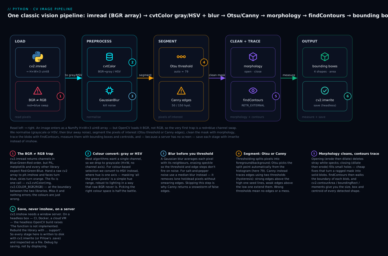
The badges mark the six places beginners get hurt: the BGR≠RGB swap at load (1), choosing grayscale vs HSV (2), blurring before you threshold (3), picking segmentation thresholds (4), morphology-then-contours to detect blobs (5), and saving instead of showing on a server (6). We hit each one in order.
| Pipeline stage | Typical function(s) | Input → output | What it buys you |
|---|---|---|---|
| Load | cv2.imread, Image.open |
file → H×W×3 uint8 (BGR!) |
Pixels in memory as an array |
| Colour convert | cv2.cvtColor |
BGR → gray / HSV | One channel for algorithms; hue for colour masks |
| Filter / denoise | GaussianBlur, medianBlur |
array → smoother array | Kills noise so later steps don’t misfire |
| Threshold / edges | threshold (Otsu), Canny |
gray → binary mask / edge map | Splits “interesting” pixels from background |
| Morphology | erode, dilate, morphologyEx |
mask → cleaner mask | Removes specks, fills holes |
| Contours | findContours, boundingRect |
mask → list of shapes + boxes | Detects and measures objects |
| Output | cv2.imwrite, Image.save |
array → file | Persist results (headless-safe) |
An image is a NumPy array
Load an image with OpenCV and inspect it the way you would inspect any array. A colour image is three-dimensional — (height, width, channels) — and the dtype is uint8, an unsigned 8-bit integer holding exactly 0–255. That range is not arbitrary: 0 is “no light in this channel,” 255 is “full brightness,” and 8 bits is what camera sensors and display hardware settled on decades ago.
import cv2
import numpy as np

# synthesize a 120x240 colour image: three vertical blocks
img = np.zeros((120, 240, 3), dtype=np.uint8)   # (H, W, C) of zeros = black
img[:, :80]    = (0, 0, 255)   # left  block
img[:, 80:160] = (0, 255, 0)   # middle block
img[:, 160:]   = (255, 0, 0)   # right block
cv2.imwrite("blocks.png", img)   # write to disk (headless-safe)

print(type(img).__name__)   # ndarray      -- it's just a NumPy array
print(img.shape)            # (120, 240, 3)  H=120 rows, W=240 cols, 3 channels
print(img.dtype)            # uint8         every pixel 0-255
print(img.min(), img.max()) # 0 255
print(img[0, 0])            # [  0   0 255]  the top-left pixel's 3 channel values
Read those attributes and you already know how to manipulate the image: it is 120 * 240 * 3 = 86,400 bytes in one contiguous buffer, indexed as img[row, col, channel]. Slicing works exactly as it does for any array — img[:, :80] is “all rows, first 80 columns,” a view onto the same buffer (the aliasing rule from the NumPy lesson applies: mutate a slice, mutate the original). A pixel is a length-3 vector; a row is a (240, 3) array; the whole thing is a stack you can broadcast over.
| Attribute | Colour image | Grayscale image | Meaning |
|---|---|---|---|
shape |
(H, W, 3) |
(H, W) |
Grid size; colour has a channel axis, gray does not |
ndim |
3 |
2 |
Number of axes |
dtype |
uint8 |
uint8 |
0–255 per channel |
img[y, x] |
[b, g, r] (3 values) |
one scalar | A single pixel |
img[y, x, 0] |
one channel value | — | Indexing into the channel axis |
img.size |
H*W*3 |
H*W |
Total byte count |
Grayscale drops the channel axis
Convert to grayscale and the channel axis disappears — a grayscale image is genuinely two-dimensional, (H, W), one intensity per pixel. This trips people constantly: code that indexes img[y, x, 0] explodes the moment the image is grayscale, because there is no third axis to index.
gray = cv2.cvtColor(img, cv2.COLOR_BGR2GRAY)
print(gray.shape)   # (120, 240)   NO channel axis -- it's 2-D
print(gray.ndim)    # 2
print(gray[10, 10], gray[10, 100], gray[10, 200])   # 76 150 29
Those three numbers — 76 150 29 — are the grayscale values of the red, green and blue blocks, and they reveal how grayscale is computed. It is not the average of the channels; it is a luminosity-weighted sum, Y = 0.299·R + 0.587·G + 0.114·B, because human eyes are far more sensitive to green than to blue. Pure red (255) becomes 0.299 × 255 ≈ 76, pure green becomes 0.587 × 255 ≈ 150, pure blue only 0.114 × 255 ≈ 29. Green looks brightest to us, so it dominates the gray value.
The dtype matters — a lot
Because pixels are uint8, all the dtype pitfalls from NumPy apply, and one bites immediately: uint8 arithmetic wraps around. 255 + 10 is not 265 (which doesn’t fit in 8 bits) — it wraps modulo 256 to 9. Brighten an image with plain + and the bright regions turn dark.
px = np.array([250, 100, 50], dtype=np.uint8)
print(px + np.uint8(30))          # [ 24 130  80]   250+30 wrapped to 24!
# safe options:
print(cv2.add(px, np.array([30, 30, 30], np.uint8)))   # [255 130 80]  SATURATES at 255
print(np.clip(px.astype(np.int16) + 30, 0, 255).astype(np.uint8))  # [255 130 80]
cv2.add saturates (clamps at 0 and 255) instead of wrapping, which is almost always what you want for image math. The other safe pattern is to widen to int16/float, do the arithmetic, np.clip to [0, 255], and cast back to uint8. We return to this in troubleshooting because it is the single most common “why did my filter darken the image” bug.
| dtype | Range | Where it shows up | Danger |
|---|---|---|---|
uint8 |
0–255 | The default for loaded images | Wraps on overflow; must clip |
uint16 |
0–65535 | 16-bit medical / RAW images | Rarely displayed directly |
float32 |
any | After normalising to [0,1] for ML |
Must scale back to uint8 to save |
float64 |
any | Intermediate math (blur, warp) | imwrite truncates; PIL refuses it |
The BGR-vs-RGB gotcha
This one deserves its own section because it wastes more beginner hours than any algorithm. OpenCV loads and stores images in B, G, R channel order — blue first — for historical reasons (the Windows bitmap format it grew up with). Almost everything else in the Python world — Pillow, matplotlib, imageio, PyTorch, the entire web — uses R, G, B. So the instant you move an image between OpenCV and any other library without converting, red and blue swap: skies go orange, faces go blue, and no error is raised because the array shape is identical.
Watch the swap happen with real pixel values. The same red pixel is [0, 0, 255] in OpenCV’s BGR and [255, 0, 0] in RGB — the channels are literally reversed:
loaded = cv2.imread("blocks.png")     # OpenCV gives you BGR
print(loaded[10, 10])                  # [  0   0 255]   a RED pixel, stored B=0 G=0 R=255

rgb = cv2.cvtColor(loaded, cv2.COLOR_BGR2RGB)   # THE FIX
print(rgb[10, 10])                     # [255   0   0]   same pixel, now R=255 G=0 B=0
print(np.array_equal(loaded[..., ::-1], rgb))   # True   BGR->RGB is just reversing channels
cv2.cvtColor(img, cv2.COLOR_BGR2RGB) is the fix, and since the conversion is just a channel reversal you will also see the NumPy shortcut img[..., ::-1]. The rule to internalise: convert at the boundary. Keep images in BGR while you are inside OpenCV, and convert to RGB only when you hand the array to Pillow, matplotlib, or a model. If you are using matplotlib to display an image, plt.imshow expects RGB — feed it a raw cv2 array and you get the blue-face bug in its purest form.
import matplotlib
matplotlib.use("Agg")            # headless backend: render to file, no window
import matplotlib.pyplot as plt

fig, ax = plt.subplots(1, 2, figsize=(6, 2))
ax[0].imshow(loaded); ax[0].set_title("cv2 array, WRONG")   # blue<->red swapped
ax[1].imshow(rgb);    ax[1].set_title("cvtColor, right")
plt.savefig("bgr_vs_rgb.png")    # save, don't plt.show() on a server
| Library | Channel order | Array shape | Notes |
|---|---|---|---|
OpenCV (cv2) |
BGR | (H, W, 3) |
The odd one out; convert on the way out |
Pillow (PIL) |
RGB | via np.asarray → (H, W, 3) |
.size is (W, H) — transposed! |
| matplotlib | RGB | expects (H, W, 3) or (H, W) |
imshow shows blue faces if fed BGR |
| PyTorch / TF | RGB | often (C, H, W) |
Also transposes the channel axis to the front |
| NumPy raw | whatever you put | (H, W, C) |
img[..., ::-1] flips channel order |
Pillow vs OpenCV: two libraries, two jobs
Python has two dominant image libraries and they are good at different things. Pillow (PIL) is the friendly, Pythonic one: open a file, resize it, crop it, convert its format, save it. It thinks in Image objects and (width, height). OpenCV (cv2) is the computer-vision workhorse: thresholding, edges, contours, camera calibration, optical flow, and thousands of algorithms Pillow has never heard of. It thinks in NumPy arrays and (height, width). Most real projects use both — Pillow for I/O and simple transforms, OpenCV for the vision.
Pillow (PIL) |
OpenCV (cv2) |
|
|---|---|---|
| Mental model | Image object |
NumPy ndarray |
| Dimension order | img.size = (W, H) |
img.shape = (H, W, C) |
| Channel order | RGB | BGR |
| Strengths | Open/save, format conversion, resize, crop, rotate, thumbnails, EXIF, text | Filtering, thresholding, edges, contours, morphology, video, ML preprocessing |
| Weaknesses | No CV algorithms | Clunky I/O, no format niceties |
| Install | pip install pillow |
pip install opencv-python-headless |
| Grayscale | .convert("L") → 2-D |
cvtColor(..., BGR2GRAY) → 2-D |
| Typical role | Load / save / simple edits | The vision pipeline |
Pillow: the I/O and simple-edits toolkit
Pillow’s API reads like plain English. Image.open is lazy — it reads the header (size, format) but not the pixels until you actually need them, which makes opening a directory of thumbnails cheap.
from PIL import Image, ImageOps

im = Image.open("blocks.png")
print(im.size, im.mode, im.format)   # (240, 120) RGB PNG   <- size is (W, H)!

im.resize((200, 150))                # (W, H) -- note the order
im.crop((40, 40, 140, 160))          # box = (left, top, right, bottom) -> 100x120
im.rotate(30, expand=True)           # rotate CCW; expand grows the canvas to fit
thumb = im.copy(); thumb.thumbnail((100, 100))   # IN PLACE, preserves aspect ratio
print(thumb.size)                    # (100, 50)   fit inside 100x100, aspect kept
im.convert("L").save("gray.png")     # to grayscale, then save
im.save("out.jpg", quality=85)       # format inferred from extension
The (W, H) versus (H, W) disagreement between Pillow and NumPy is a genuine trap: im.size is (width, height) but np.asarray(im).shape is (height, width, channels). When you convert between them, the two numbers swap places.
| Pillow method | Does | Argument order |
|---|---|---|
Image.open(path) |
Lazily open (reads header only) | — |
im.size |
(width, height) |
note: not (H, W) |
im.resize((w, h)) |
Resize to exact size | (W, H) |
im.crop((l, t, r, b)) |
Crop to a box | left, top, right, bottom |
im.rotate(deg, expand=) |
Rotate CCW; expand fits canvas |
degrees |
im.thumbnail((w, h)) |
Shrink in place, keep aspect | max box |
im.convert("L") / "RGB" / "RGBA" |
Change mode/channels | mode string |
im.transpose(Image.Transpose.FLIP_LEFT_RIGHT) |
Flip / rotate by 90° steps | enum constant |
im.save(path, quality=) |
Save; format from extension | — |
ImageOps.exif_transpose(im) |
Apply the EXIF orientation tag | — |
EXIF orientation is worth a warning. Phone cameras almost always store pixels in one physical orientation and add an EXIF tag saying “rotate this 90° when displaying.” If you read the raw pixels and ignore the tag, portrait photos come out sideways. ImageOps.exif_transpose(im) bakes the tag into the pixels so the array matches what a human sees — call it right after Image.open on any photo from a real camera.
Formats and modes: lossy, lossless, alpha
A big part of Pillow’s job is format conversion, and the format you save to is a real decision, not a cosmetic one. PNG is lossless and keeps an alpha (transparency) channel — the right choice for masks, screenshots, line art, and anything with sharp edges or text. JPEG is lossy and has no alpha — right for photographs, wrong for masks (its block compression smears hard edges, and it will flatly refuse an RGBA image). WebP does both lossy and lossless with alpha at smaller sizes, and is the sensible modern default for the web. Saving is just choosing an extension; Pillow infers the encoder.
im.save("out.png")                  # lossless, keeps alpha
im.save("out.jpg", quality=85)      # lossy; quality 1-95; NO alpha channel
im.convert("RGB").save("out.webp")  # modern: small files, optional alpha
im.convert("RGBA").save("bad.jpg")  # OSError: cannot write mode RGBA as JPEG
That last line is a real traceback (OSError: cannot write mode RGBA as JPEG) and a common trip-up: convert to RGB before saving a transparent image as JPEG, or it errors.
| Format | Compression | Alpha | Best for | Avoid for |
|---|---|---|---|---|
| PNG | Lossless | Yes | Masks, screenshots, text, line art | Huge photos (large files) |
| JPEG | Lossy | No | Photographs | Masks, sharp edges, transparency |
| WebP | Lossy or lossless | Yes | Web images (small + alpha) | Very old viewers |
| BMP | None | No | Quick debugging dumps | Anything shipped (uncompressed) |
| TIFF | Lossless/none | Yes | Scientific, archival, 16-bit | The web |
Pillow tracks channel layout with a mode string, and convert() moves between modes. The mode decides the shape you get back from np.asarray, so it is the first thing to check when an array’s shape surprises you.
| PIL mode | Meaning | np.asarray shape |
|---|---|---|
"L" |
8-bit grayscale | (H, W) |
"RGB" |
3-channel colour | (H, W, 3) |
"RGBA" |
Colour + alpha | (H, W, 4) |
"P" |
Palette (indexed colour) | (H, W) of indices |
"1" |
1-bit bilevel (black/white) | (H, W) |
Reading, writing, and the headless imshow reality
OpenCV reads and writes with imread/imwrite, and both have sharp edges. imread returns a BGR array; you can force grayscale at load time with a flag. Crucially, imread does not raise on a bad path — it returns None, and the crash comes later when you use the None:
img = cv2.imread("typo.png")     # file doesn't exist
print(img is None)               # True   -- NO exception here
print(img.shape)                 # AttributeError: 'NoneType' object has no attribute 'shape'
Always guard imread with if img is None: raise FileNotFoundError(path). This is the number-one “why is my traceback pointing at the wrong line” bug in OpenCV.
| Call | Returns | Note |
|---|---|---|
cv2.imread(path) |
BGR (H,W,3) uint8, or None |
Default IMREAD_COLOR; drops alpha |
cv2.imread(path, cv2.IMREAD_GRAYSCALE) |
(H,W) uint8 |
Load straight to gray |
cv2.imread(path, cv2.IMREAD_UNCHANGED) |
Keeps alpha → (H,W,4) |
For PNGs with transparency |
cv2.imwrite(path, img) |
True/False |
Format from extension; needs uint8 |
Image.open(path) |
PIL Image (lazy, RGB) |
.load() to force-read |
im.save(path) |
— | Format from extension |
Now the part that surprises everyone deploying to production: cv2.imshow needs a graphical window server, and servers don’t have one. On your laptop imshow pops a window; in Docker, CI, or a cloud VM there is no display, and the headless OpenCV build (the opencv-python-headless package, which you should install on servers) raises:
cv2.error: OpenCV(4.x) .../highgui/src/window.cpp: error: (-2:Unspecified error)
The function is not implemented. Rebuild the library with Windows, GTK+ 2.x or
Cocoa support. If you are on Ubuntu or Debian, install libgtk2.0-dev and
pkg-config, then re-run cmake ... in function 'cvShowImage'
The fix is not to install a GUI — it is to stop trying to display and start saving. Every debugging step becomes cv2.imwrite("stage_03_edges.png", edges), and you open the files. That is why this entire lesson is headless: it is how vision code runs where it matters. (On some desktop builds imshow may silently pop a window even from the “headless” wheel — but never rely on it; write your code to save, and it runs everywhere.)
⚠️ Install
opencv-python-headless, notopencv-python, on any server or CI runner. The two packages conflict if both are installed; pick one. The headless build is smaller, has no GUI dependencies, and forces the save-don’t-show discipline you want anyway.
Moving arrays between the libraries
Because both libraries ultimately speak NumPy, you convert freely — but you must fix the channel order at every crossing. np.asarray(pil_image) gives an RGB array; Image.fromarray(array) expects RGB. So the round-trip from OpenCV to Pillow and back is always a cvtColor sandwich:
cv = cv2.imread("blocks.png")                       # BGR array
pil = Image.fromarray(cv2.cvtColor(cv, cv2.COLOR_BGR2RGB))   # -> RGB for PIL
back = cv2.cvtColor(np.asarray(pil), cv2.COLOR_RGB2BGR)      # -> BGR for cv2

# proof the same red pixel differs by channel order:
print(pil.getpixel((10, 10)))   # (255, 0, 0)    PIL: R, G, B
print(cv[10, 10])               # [  0   0 255]   cv2: B, G, R  (reversed)
Geometric operations
Geometry — resize, crop, flip, rotate, warp — is where you prepare an image for a model (which wants a fixed input size) or correct for how it was captured. Two ideas carry all of it: crop is just NumPy slicing, and resize forces you to choose an interpolation — the rule for inventing pixel values that didn’t exist before.
Resize and the interpolation choice
When you shrink or grow an image, the new pixel grid doesn’t line up with the old one, so OpenCV must interpolate. The flag you pass changes both speed and quality, and — critically — the right choice differs for shrinking versus growing.
img = cv2.imread("blocks.png")
print(img.shape)                                        # (120, 240, 3)

big  = cv2.resize(img, (480, 240), interpolation=cv2.INTER_CUBIC)   # (W, H)!
small = cv2.resize(img, None, fx=0.5, fy=0.5, interpolation=cv2.INTER_AREA)
print(big.shape, small.shape)                           # (240, 480, 3) (60, 120, 3)
Note the trap already lurking: cv2.resize takes the target size as (width, height), the opposite of shape’s (height, width). Passing img.shape[:2] directly gives you a transposed image.
| Interpolation flag | Speed | Quality | Use for |
|---|---|---|---|
INTER_NEAREST |
Fastest | Blocky | Masks/labels (must not blend classes) |
INTER_LINEAR |
Fast | Good | The default; general resizing |
INTER_AREA |
Medium | Best when shrinking | Downscaling (avoids moiré/aliasing) |
INTER_CUBIC |
Slow | Smooth when growing | Upscaling, 4×4 neighbourhood |
INTER_LANCZOS4 |
Slowest | Sharpest | High-quality upscaling, 8×8 |
You can see the difference by upscaling a tiny image and counting how many distinct gray levels appear. INTER_NEAREST just copies existing values (few levels, blocky); the smooth methods invent in-between values (many levels, gradients):
gray = cv2.cvtColor(img, cv2.COLOR_BGR2GRAY)
tiny = cv2.resize(gray, (20, 15), interpolation=cv2.INTER_AREA)
for name, flag in [("NEAREST", cv2.INTER_NEAREST), ("LINEAR", cv2.INTER_LINEAR),
                   ("CUBIC", cv2.INTER_CUBIC), ("LANCZOS4", cv2.INTER_LANCZOS4)]:
    up = cv2.resize(tiny, (400, 300), interpolation=flag)
    print(f"{name:9s} distinct gray levels: {len(np.unique(up))}")
# NEAREST   distinct gray levels: 39
# LINEAR    distinct gray levels: 129
# CUBIC     distinct gray levels: 160
# LANCZOS4  distinct gray levels: 164
One hard rule: for a label/segmentation mask, always use INTER_NEAREST. A mask’s pixel values are class IDs (0=background, 1=cat, 2=dog); blending them with INTER_LINEAR produces a meaningless 1.5 that belongs to no class.
Crop, flip, rotate, and affine/perspective warps
Cropping needs no special function — it is a slice, img[y0:y1, x0:x1], and (being a basic slice) it returns a view, so .copy() it if you plan to draw on the crop without touching the original. Flipping mirrors along an axis. Rotation and general warps go through warpAffine (which takes a 2×3 matrix) and warpPerspective (a 3×3 matrix), because any rotate/scale/shear/translate is one matrix multiply per pixel coordinate.
crop  = img[20:100, 40:200]           # a VIEW: rows 20-99, cols 40-199 -> (80, 160, 3)
flip_h = cv2.flip(img, 1)             # 1=horizontal, 0=vertical, -1=both
flip_v = cv2.flip(img, 0)

h, w = img.shape[:2]
M = cv2.getRotationMatrix2D((w/2, h/2), 30, 1.0)   # centre, 30 deg CCW, scale 1.0
rotated = cv2.warpAffine(img, M, (w, h))           # M is 2x3
print(M.shape, rotated.shape)                      # (2, 3) (120, 240, 3)

# perspective: map 4 source corners to 4 destination corners (a 3x3 matrix)
src = np.float32([[0,0],[w,0],[0,h],[w,h]])
dst = np.float32([[20,10],[w-10,0],[0,h-5],[w-30,h-20]])
P = cv2.getPerspectiveTransform(src, dst)
warped = cv2.warpPerspective(img, P, (w, h))
print(P.shape)                                     # (3, 3)
Perspective warps are how you “de-skew” a photographed document: pick its four corners as src, map them to a clean rectangle as dst, and warpPerspective flattens it.
Both warps rest on one idea: a transformation matrix maps each output pixel’s coordinate back to a source coordinate, and OpenCV interpolates the colour there. An affine 2×3 matrix can translate, scale, rotate and shear, and it always keeps parallel lines parallel; a perspective 3×3 matrix additionally lets parallel lines converge, which is exactly what creates the illusion of depth (railway tracks meeting at the horizon). You almost never build these matrices by hand — helpers like getRotationMatrix2D and getPerspectiveTransform construct them — but knowing which one you need tells you which warp* function to call.
| Transform | Matrix | Keeps parallel lines? | Built by |
|---|---|---|---|
| Translate | 2×3 | Yes | Manual [[1,0,tx],[0,1,ty]] |
| Scale | 2×3 | Yes | [[sx,0,0],[0,sy,0]] |
| Rotate (about a point) | 2×3 | Yes | getRotationMatrix2D(c, deg, scale) |
| General affine | 2×3 | Yes | getAffineTransform(3 pts → 3 pts) |
| Perspective | 3×3 | No (they converge) | getPerspectiveTransform(4 pts → 4 pts) |
| Operation | Function | Key parameter |
|---|---|---|
| Crop | img[y0:y1, x0:x1] (slice) |
Returns a view |
| Resize | cv2.resize(img, (w, h), interpolation=) |
Size is (W, H) |
| Flip | cv2.flip(img, code) |
1=horiz, 0=vert, -1=both |
| Rotate 90° | cv2.rotate(img, cv2.ROTATE_90_CLOCKWISE) |
Lossless, no interpolation |
| Rotate any angle | warpAffine(img, getRotationMatrix2D(c, a, s), (w,h)) |
2×3 matrix |
| Translate/shear/scale | warpAffine(img, M, (w,h)) |
Any 2×3 affine M |
| Perspective | warpPerspective(img, getPerspectiveTransform(src,dst), (w,h)) |
3×3 matrix |
Colour spaces and thresholding
To find things by colour, raw BGR is a poor coordinate system: change the lighting and all three channels move together, so “green” spans a huge, awkward BGR region. HSV — Hue, Saturation, Value — fixes this by putting colour on one axis (hue) and brightness on another (value). “All the green pixels, whatever the lighting” becomes a simple hue range, which is why HSV is the standard space for colour-based masking.
hsv = cv2.cvtColor(img, cv2.COLOR_BGR2HSV)
print(hsv[10, 10], hsv[10, 100], hsv[10, 200])   # [0 255 255] [60 255 255] [120 255 255]
Mind OpenCV’s HSV ranges, which are non-obvious because they are squeezed into uint8: Hue is 0–179 (degrees halved, since 360 won’t fit in a byte), while Saturation and Value are 0–255. Red sits at hue 0, green at 60, blue at 120 — half their usual degree values.
cv2.inRange builds a binary mask (255 where the pixel falls inside the HSV bounds, 0 elsewhere), and that mask is how you select or count colour:
lower = np.array([40, 50, 50])     # low green: hue 40, some saturation/brightness
upper = np.array([80, 255, 255])   # high green: hue 80
mask = cv2.inRange(hsv, lower, upper)
print(mask.shape, np.unique(mask))          # (120, 240) [  0 255]   a 2-D binary mask
print(int((mask > 0).sum()), "green px")    # 9600 green px
# apply the mask to keep only the green region:
green_only = cv2.bitwise_and(img, img, mask=mask)
One colour breaks the “single range” convenience: red wraps around the hue circle. Red sits at hue 0, but because the circle joins 179 back to 0, red pixels land at both ends — roughly hue 0–10 and 170–179. A single inRange can’t span that gap, so to mask red you build two masks and OR them: cv2.inRange(hsv,(0,120,70),(10,255,255)) | cv2.inRange(hsv,(170,120,70),(179,255,255)). Every other colour is one contiguous band; only red needs the two-piece treatment.
| Colour space | cvtColor code |
Axes | Best for |
|---|---|---|---|
| Grayscale | COLOR_BGR2GRAY |
intensity | Most algorithms (edges, threshold) |
| RGB | COLOR_BGR2RGB |
R, G, B | Handing off to PIL/matplotlib/ML |
| HSV | COLOR_BGR2HSV |
H 0-179, S 0-255, V 0-255 | Colour-based masking |
| LAB | COLOR_BGR2LAB |
L, a, b | Perceptual colour distance |
| HLS | COLOR_BGR2HLS |
H, L, S | Alternative to HSV |
Thresholding: binary, Otsu, adaptive
Thresholding turns a grayscale image into a black-and-white mask: pixels above a cutoff become 255, the rest 0. The question is what cutoff, and there are three answers. A fixed threshold is a number you pick. Otsu picks the number for you by finding the split that best separates the histogram’s two peaks — ideal when foreground and background are distinct. Adaptive computes a different threshold for each small region, which is the only thing that works under uneven lighting.
gray = cv2.cvtColor(img, cv2.COLOR_BGR2GRAY)

# fixed: everything brighter than 100 -> white
t1, binary = cv2.threshold(gray, 100, 255, cv2.THRESH_BINARY)
print(t1, np.unique(binary))          # 100.0 [  0 255]

# Otsu: pass 0 as the threshold and add the flag; it RETURNS the value it chose
t2, otsu = cv2.threshold(gray, 0, 255, cv2.THRESH_BINARY + cv2.THRESH_OTSU)
print("Otsu picked:", t2)             # Otsu picked: 76.0

# adaptive: per-region threshold, for uneven illumination
adaptive = cv2.adaptiveThreshold(gray, 255, cv2.ADAPTIVE_THRESH_GAUSSIAN_C,
                                 cv2.THRESH_BINARY, blockSize=11, C=2)
The most useful is Otsu: give it 0 for the threshold, add THRESH_OTSU, and it returns the cutoff it computed from the data — no magic number to tune. It assumes a bimodal histogram (two clear peaks), so it shines on “dark objects on a light background” and struggles on smooth gradients.
| Method | Call | Threshold source | Use when |
|---|---|---|---|
| Fixed binary | threshold(g, T, 255, THRESH_BINARY) |
You pick T |
You know the cutoff |
| Inverse | THRESH_BINARY_INV |
You pick T |
Dark objects, light background |
| Otsu | threshold(g, 0, 255, THRESH_BINARY+THRESH_OTSU) |
Auto (from histogram) | Bimodal, even lighting |
| Adaptive | adaptiveThreshold(g, 255, ...) |
Per-region | Uneven lighting, documents |
| To-zero | THRESH_TOZERO |
You pick T |
Keep bright values, zero the rest |
Filtering, convolution, and the bridge to CNNs
Filtering is how you smooth, sharpen, or extract features, and every filter here is a convolution: slide a small grid of weights (a kernel) over the image, and at each position compute the weighted sum of the neighbourhood. Change the weights and you change the effect. This is not an analogy for what a convolutional neural network does — it is literally the same operation. A CNN’s “learned filters” are kernels exactly like these, except the network discovers the weights instead of you writing them. Master hand-built kernels here and the next step into deep learning is a short one.
Blur: Gaussian for general noise, median for salt-and-pepper
A Gaussian blur replaces each pixel with a weighted average of its neighbours (nearby pixels count more), smoothing out fine noise. It is the standard “denoise before you threshold or detect edges” step. But for salt-and-pepper noise — random pure-white and pure-black specks — a Gaussian smears the specks instead of removing them; you want a median blur, which replaces each pixel with the median of its neighbourhood, and a lone white speck is never the median, so it vanishes.
# a clean scene, then salt & pepper noise added
scene = cv2.imread("scene.png")            # (built in the lab below)
noisy = scene.copy()
# ... sprinkle 2000 white + 2000 black pixels ...

median = cv2.medianBlur(noisy, 5)          # ksize must be ODD
gauss  = cv2.GaussianBlur(noisy, (5, 5), 0)  # (kernel W,H) odd; sigma 0 = auto

# mean abs difference from the clean original (lower = better denoise):
def mad(a, b): return float(np.abs(a.astype(int) - b.astype(int)).mean())
print("noisy :", round(mad(noisy,  scene), 2))    # 4.17
print("median:", round(mad(median, scene), 2))    # 0.04   <- median crushes s&p noise
print("gauss :", round(mad(gauss,  scene), 2))    # 4.62   <- barely helps here
The numbers are decisive: median blur drops the error from 4.17 to 0.04 on salt-and-pepper noise, while Gaussian barely moves it. Matching the filter to the noise is the whole skill.
Two knobs control every blur. Kernel size must be odd (3, 5, 7, …) so it has a well-defined centre pixel; a bigger kernel averages more neighbours and smooths harder, at the cost of detail and speed. For GaussianBlur, a sigma of 0 tells OpenCV to derive the spread from the kernel size. And when you need to remove noise but keep edges crisp — smoothing a portrait’s skin without blurring the eyes — reach for cv2.bilateralFilter, which weights neighbours by both distance and colour similarity, so it refuses to average across a strong edge. It is slower than a Gaussian but the only one-shot filter that denoises without softening boundaries.
| Filter | Function | Kernel | Best for |
|---|---|---|---|
| Gaussian blur | GaussianBlur(img, (k,k), sigma) |
Bell-shaped weights | General noise; pre-edge smoothing |
| Median blur | medianBlur(img, k) |
Median of neighbourhood | Salt-and-pepper noise |
| Box/mean blur | blur(img, (k,k)) |
Uniform average | Fast, crude smoothing |
| Bilateral | bilateralFilter(img, d, sc, ss) |
Edge-aware | Denoise while keeping edges |
| Custom | filter2D(img, -1, kernel) |
Any weights you supply | Sharpen, emboss, feature detect |
A kernel is just a weight matrix (this is a conv layer)
cv2.filter2D lets you supply any kernel, which makes the CNN connection concrete. A 3×3 box of 1/9 averages (blur); a centre-heavy kernel sharpens; a left-minus-right kernel detects vertical edges. Prove to yourself that convolution is exactly a sliding weighted sum:
box     = np.ones((3, 3), np.float32) / 9.0            # average of 9 -> blur
sharpen = np.array([[0,-1,0],[-1,5,-1],[0,-1,0]], np.float32)   # centre-surround
sobel_x = np.array([[-1,0,1],[-2,0,2],[-1,0,1]], np.float32)    # vertical-edge detector

blurred = cv2.filter2D(gray, -1, box)
edges_x = cv2.filter2D(gray, -1, sobel_x)

# the box filter at a pixel == the plain mean of its 3x3 neighbourhood:
y, x = 100, 90
print("manual 3x3 mean:", round(float(gray[y-1:y+2, x-1:x+2].mean()), 1))  # 135.0
print("filter2D value :", int(blurred[y, x]))                              # 135
The manual mean and filter2D agree exactly (135), because that is all convolution is: a weighted neighbourhood sum, one per pixel. A CNN stacks thousands of these and learns the weights — sobel_x is a hand-designed edge detector; a trained network derives similar filters on its own in its first layer.
Edge detection with Canny
Edges — sharp intensity changes — are where objects meet background, and Canny is the classic detector. It takes two thresholds and uses hysteresis: pixels with gradient above the high threshold are definite edges; pixels above the low threshold are edges only if they connect to a definite one. This two-level scheme traces continuous contours while rejecting isolated noise.
blur = cv2.GaussianBlur(gray, (7, 7), 0)   # ALWAYS blur first
edges = cv2.Canny(blur, 50, 150)           # (low, high) thresholds
print(edges.shape, np.unique(edges), int((edges>0).sum()))  # (120,240) [0 255] ...
Getting the two thresholds wrong is the usual Canny failure, in both directions. Too high and real edges vanish; too low (especially without blurring first) and noise floods the output with spurious edges:
# too high -> misses edges;  too low on a noisy image -> noise storm
print(int((cv2.Canny(blur, 240, 250) > 0).sum()))   # 496    (too high: barely any edges)
noisy_gray = np.clip(gray + rng.normal(0, 25, gray.shape), 0, 255).astype(np.uint8)
print(int((cv2.Canny(noisy_gray, 10, 30) > 0).sum()))  # 44194  (too low: noise flood)
Canny’s own advice is a high:low ratio of 2:1 or 3:1, and to always blur first. Start with something like Canny(blur, 50, 150) and adjust.
| Canny knob | Effect | Symptom if wrong |
|---|---|---|
| Low threshold | Weak-edge floor (hysteresis) | Too low → noisy edges everywhere |
| High threshold | Strong-edge seed | Too high → broken/missing edges |
| Blur first | Removes noise before gradients | Skip it → snowstorm of false edges |
apertureSize |
Sobel kernel size (3/5/7) | Larger = thicker gradient response |
Morphology and contours
After thresholding you have a binary mask, but it is rarely clean: a few stray white specks, a few black pinholes inside solid shapes. Morphology fixes this with two primitives operating on white regions — erode (shrink white) and dilate (grow white) — and their two useful combinations. Opening (erode then dilate) removes small white specks without shrinking big shapes; closing (dilate then erode) fills small black holes without growing shapes.
kernel = np.ones((5, 5), np.uint8)          # the structuring element
eroded  = cv2.erode(binary, kernel, iterations=1)
dilated = cv2.dilate(binary, kernel, iterations=1)
opened  = cv2.morphologyEx(binary, cv2.MORPH_OPEN,  kernel)   # de-speckle
closed  = cv2.morphologyEx(binary, cv2.MORPH_CLOSE, kernel)   # fill holes

print("white px  binary:", int((binary>0).sum()))    # 34324
print("white px  erode :", int((eroded>0).sum()))     # 31268  (shrank)
print("white px  dilate:", int((dilated>0).sum()))    # 37508  (grew)
The pixel counts confirm the intuition: erode drops white pixels (34324 → 31268), dilate adds them (→ 37508). Opening’s power shows on a speckled mask — sprinkle 194 tiny white blobs and opening deletes essentially all of them while leaving the real shapes:
# speckled mask has 194 connected components; opening removes the specks
n_before, _ = cv2.connectedComponents(speckled)
n_after,  _ = cv2.connectedComponents(cv2.morphologyEx(speckled, cv2.MORPH_OPEN, kernel))
print(n_before - 1, "->", n_after - 1)   # 194 -> 4   (specks gone, 4 shapes remain)
| Morphology op | morphologyEx flag |
Effect | Use for |
|---|---|---|---|
| Erode | cv2.erode |
Shrinks white regions | Separate touching blobs, thin |
| Dilate | cv2.dilate |
Grows white regions | Connect gaps, thicken |
| Opening | MORPH_OPEN (erode→dilate) |
Removes small white specks | De-noise a mask |
| Closing | MORPH_CLOSE (dilate→erode) |
Fills small black holes | Solidify shapes |
| Gradient | MORPH_GRADIENT |
Dilate − erode | Outline / edge of blobs |
| Top hat | MORPH_TOPHAT |
Image − opening | Bright detail on dark bg |
Contours: find, measure, and box the shapes
A contour is the boundary curve of a connected white region. cv2.findContours walks your cleaned mask and returns a list of these curves; each one is an object you can measure. RETR_EXTERNAL keeps only outermost contours (ignore holes); CHAIN_APPROX_SIMPLE compresses straight runs to their endpoints to save memory.
contours, hierarchy = cv2.findContours(closed, cv2.RETR_EXTERNAL, cv2.CHAIN_APPROX_SIMPLE)
print(len(contours), "shapes found")        # 4 shapes found

for c in sorted(contours, key=cv2.contourArea, reverse=True):
    area = cv2.contourArea(c)               # pixels enclosed
    x, y, w, h = cv2.boundingRect(c)        # upright box (x, y, width, height)
    M = cv2.moments(c)                      # spatial moments
    cx, cy = int(M["m10"]/M["m00"]), int(M["m01"]/M["m00"])   # centroid
    print(f"area={int(area):6d}  bbox=({x},{y},{w},{h})  centroid=({cx},{cy})")
# area= 11998  bbox=(40,40,101,121)   centroid=(90,100)
# area=  9452  bbox=(245,35,111,111)  centroid=(300,90)
# area=  7342  bbox=(251,201,109,69)  centroid=(305,235)
# area=  4868  bbox=(71,201,79,79)    centroid=(110,240)
The centroid comes from image moments: m00 is the area, and (m10/m00, m01/m00) is the centre of mass. That is genuinely all “object detection” is at this classical level — threshold, clean, contour, measure. A modern neural detector replaces these four steps with one learned model, but the outputs (a box and a centre per object) are identical, which is why understanding this makes the ML version legible.
| Contour tool | Call | Returns |
|---|---|---|
| Find contours | findContours(mask, mode, method) |
(contours, hierarchy) |
| Retrieval mode | RETR_EXTERNAL / RETR_TREE / RETR_LIST |
Outer only / nested / flat |
| Area | cv2.contourArea(c) |
Enclosed pixel count |
| Perimeter | cv2.arcLength(c, closed=True) |
Boundary length |
| Upright box | cv2.boundingRect(c) |
(x, y, w, h) |
| Rotated box | cv2.minAreaRect(c) |
((cx,cy),(w,h),angle) |
| Centroid | cv2.moments(c) → m10/m00, m01/m00 |
Centre of mass |
| Convex hull | cv2.convexHull(c) |
Smallest enclosing polygon |
| Draw | cv2.drawContours(img, contours, -1, colour, t) |
In place |
The two flags to findContours decide which contours come back and how densely each is stored. Pick the wrong retrieval mode and holes inside a shape return as separate objects (or vanish); pick CHAIN_APPROX_NONE and you store every boundary pixel instead of just the corners.
| Flag | Category | Meaning |
|---|---|---|
RETR_EXTERNAL |
Retrieval | Outermost contours only (ignore holes) |
RETR_LIST |
Retrieval | All contours, flat (no hierarchy) |
RETR_CCOMP |
Retrieval | Two levels: outer boundaries + holes |
RETR_TREE |
Retrieval | Full nested parent/child hierarchy |
CHAIN_APPROX_NONE |
Approximation | Every boundary point (memory-heavy) |
CHAIN_APPROX_SIMPLE |
Approximation | Compress straight runs to endpoints |
Drawing: annotate what you found
To visualise detections you draw straight onto the array. All the drawing functions modify the image in place, take BGR colours, and use (x, y) (column, row) coordinates — the opposite order to array indexing, another easy slip.
annot = scene.copy()
for c in contours:
    x, y, w, h = cv2.boundingRect(c)
    cv2.rectangle(annot, (x, y), (x+w, y+h), (0, 255, 255), 2)   # yellow box, thickness 2
    cv2.circle(annot, (x+w//2, y+h//2), 4, (255, 255, 255), -1)  # -1 = filled
    cv2.putText(annot, "shape", (x, y-6), cv2.FONT_HERSHEY_SIMPLEX,
                0.5, (255, 255, 255), 1, cv2.LINE_AA)
cv2.imwrite("annotated.png", annot)        # save, don't show
Histograms and contrast
A histogram counts how many pixels sit at each intensity — the shape of an image’s tonal distribution. A low-contrast image has all its counts bunched in a narrow band; histogram equalization stretches that band across the full 0–255 range, boosting contrast automatically.
lowc = (gray * 0.4 + 100).clip(0, 255).astype(np.uint8)   # squash into 112-163
eq   = cv2.equalizeHist(lowc)                              # stretch to full range
print("low-contrast range:", lowc.min(), "-", lowc.max(), " std", round(float(lowc.std()),1))
print("equalized    range:", eq.min(),   "-", eq.max(),   " std", round(float(eq.std()),1))
# low-contrast range: 112 - 163  std 18.7
# equalized    range: 0 - 255    std 83.9
hist = cv2.calcHist([lowc], [0], None, [256], [0, 256])   # 256-bin histogram
The standard deviation jumps from 18.7 to 83.9 — that is the contrast you gained, quantified. (For colour images, equalize the V channel in HSV, or use cv2.createCLAHE() for a local, less harsh version.)
From hand-built pipelines to learned ones
Step back and notice what you have been doing: at every stage you chose the operation — this blur, that Otsu threshold, these 5×5 morphology kernels. That is classical computer vision, and it is genuinely powerful: fast, interpretable, needs no training data, and runs on a Raspberry Pi. Its ceiling is that a human has to design each feature. The moment “find the defective solder joint” depends on a texture too subtle to write a kernel for, hand-tuning collapses.
Deep learning flips the authorship. A convolutional neural network is a stack of the very same filter2D convolutions you used above — but the kernel weights are learned from labelled examples instead of hand-set, so the network discovers the right filters (crude edge detectors in its first layer, object parts deeper in) rather than you writing them. You already built a Sobel edge detector by hand; a CNN derives similar filters on its own, then thousands more you would never think of. The trade is real: it needs data, it needs a GPU to train, and it gives up interpretability. Neither approach wins outright — production systems routinely use classical CV for the plumbing (load, denoise, crop, colour-normalise) and hand the hard perception in the middle to a network. Everything in this lesson is that plumbing; the next step into machine learning is the network that sits in the gap.
| Aspect | Classical CV (this lesson) | Deep learning (next lessons) |
|---|---|---|
| Who designs the features | You — kernels, thresholds, morphology | The network learns them from data |
| Training data | None needed | Many labelled examples |
| Compute | Runs on a CPU / edge device | A GPU to train, ideally |
| Interpretability | High — every step is explicit | Low — millions of opaque weights |
| Best at | Well-defined, geometric tasks | Messy, subtle, high-variety perception |
| Core operation | cv2.filter2D with fixed kernels |
Conv layers with learned kernels |
Hands-on lab
You will build the entire pipeline end to end on a synthesized scene, saving every stage to disk so you can open the PNGs and see what each step did. No dataset needed — the scene is generated in code, so this runs identically on your laptop or a bare server.
⚠️ Use a Python 3.12+ interpreter (macOS system Python is 3.9). Work in a virtual environment and install the headless OpenCV build:
python3.12 -m venv .venv
source .venv/bin/activate        # Windows: .venv\Scripts\activate
pip install opencv-python-headless pillow numpy
python -c "import cv2, numpy; print('cv2', cv2.__version__, '| numpy', numpy.__version__)"
# cv2 5.0.0 | numpy 2.5.1   (versions may differ)
Create cv_lab.py and add each step, running python cv_lab.py as you go. Every non-timing output below is exact.
Step 1 — Synthesize a scene and read its header.
import cv2, numpy as np, time
rng = np.random.default_rng(0)

scene = np.full((300, 400, 3), 30, dtype=np.uint8)              # dark gray background
cv2.rectangle(scene, (40, 40), (140, 160), (60, 180, 75), -1)   # green rectangle (BGR)
cv2.circle(scene, (300, 90), 55, (0, 140, 255), -1)            # orange circle
cv2.circle(scene, (110, 240), 40, (200, 60, 200), -1)          # purple circle
cv2.rectangle(scene, (250, 200), (360, 270), (40, 40, 230), -1) # red rectangle
cv2.imwrite("stage0_scene.png", scene)
print("scene:", scene.shape, scene.dtype)   # scene: (300, 400, 3) uint8
What just happened: you built a (300, 400, 3) uint8 array with four coloured shapes on a dark background — a controlled test image. The -1 thickness fills each shape. This is your ground truth: four objects to find.
Step 2 — Prove the BGR→RGB swap.
print("green pixel BGR (cv2):", scene[100, 90])                      # [ 60 180  75]
rgb = cv2.cvtColor(scene, cv2.COLOR_BGR2RGB)
print("green pixel RGB       :", rgb[100, 90])                       # [ 75 180  60]
print("just a channel flip? :", np.array_equal(scene[..., ::-1], rgb))  # True
cv2.imwrite("stage2_rgb_wrong.png", rgb)   # saving RGB as if BGR -> looks swapped
What just happened: the same green pixel is [60,180,75] in cv2’s BGR and [75,180,60] in RGB — red and blue traded places. stage2_rgb_wrong.png deliberately saves the RGB array back through cv2 (which assumes BGR), so it looks colour-swapped: proof of the bug, on disk.
Step 3 — Grayscale, then Gaussian-blur.
gray = cv2.cvtColor(scene, cv2.COLOR_BGR2GRAY)
blur = cv2.GaussianBlur(gray, (7, 7), 0)
print("gray shape:", gray.shape, "(2-D, no channel axis)")   # (300, 400)
cv2.imwrite("stage3_gray.png", gray)
cv2.imwrite("stage3_blur.png", blur)
What just happened: grayscale collapsed the 3 channels into one (300, 400) plane; the 7×7 Gaussian smoothed it so the next steps won’t fire on stray pixels. Blurring before thresholding/edges is the habit that prevents most noise bugs.
Step 4 — Otsu threshold to a binary mask.
t, binary = cv2.threshold(blur, 0, 255, cv2.THRESH_BINARY + cv2.THRESH_OTSU)
print("Otsu chose threshold:", t)                 # Otsu chose threshold: 79.0
print("mask values:", np.unique(binary), "white px:", int((binary>0).sum()))
cv2.imwrite("stage4_binary.png", binary)          # mask values: [0 255] white px: 34324
What just happened: Otsu inspected the histogram and picked 79 on its own, producing a black-and-white mask where the four shapes are white. No hand-tuned magic number — the data chose the split.
Step 5 — Morphology to clean the mask.
kernel = np.ones((5, 5), np.uint8)
clean = cv2.morphologyEx(binary, cv2.MORPH_OPEN,  kernel)   # remove specks
clean = cv2.morphologyEx(clean,  cv2.MORPH_CLOSE, kernel)   # fill holes
cv2.imwrite("stage5_clean.png", clean)
print("white px after morphology:", int((clean>0).sum()))   # 34324
What just happened: opening then closing scrubbed the mask — any speckle gone, any pinhole filled — so the contour step traces four solid blobs instead of a ragged edge.
Step 6 — Find contours, measure and box each shape.
contours, _ = cv2.findContours(clean, cv2.RETR_EXTERNAL, cv2.CHAIN_APPROX_SIMPLE)
print("shapes detected:", len(contours))          # shapes detected: 4
annot = scene.copy()
for i, c in enumerate(sorted(contours, key=cv2.contourArea, reverse=True)):
    area = cv2.contourArea(c)
    x, y, w, h = cv2.boundingRect(c)
    M = cv2.moments(c); cx, cy = int(M["m10"]/M["m00"]), int(M["m01"]/M["m00"])
    cv2.rectangle(annot, (x, y), (x+w, y+h), (0, 255, 255), 2)
    cv2.circle(annot, (cx, cy), 4, (255, 255, 255), -1)
    cv2.putText(annot, f"#{i} A={int(area)}", (x, y-6),
                cv2.FONT_HERSHEY_SIMPLEX, 0.5, (255,255,255), 1, cv2.LINE_AA)
    print(f"  #{i}: area={int(area):6d}  bbox=({x},{y},{w},{h})  centroid=({cx},{cy})")
cv2.imwrite("stage6_annotated.png", annot)
#   #0: area= 11998  bbox=(40,40,101,121)   centroid=(90,100)
#   #1: area=  9452  bbox=(245,35,111,111)  centroid=(300,90)
#   #2: area=  7342  bbox=(251,201,109,69)  centroid=(305,235)
#   #3: area=  4868  bbox=(71,201,79,79)    centroid=(110,240)
What just happened: all four shapes detected, each with a real area, bounding box, and centroid drawn onto stage6_annotated.png. The centroids (90,100), (300,90), (305,235), (110,240) match exactly where you drew the shapes. That is a complete classical object-detection pipeline.
Step 7 — HSV-mask a single colour.
hsv = cv2.cvtColor(scene, cv2.COLOR_BGR2HSV)
green_mask = cv2.inRange(hsv, np.array([40,50,50]), np.array([80,255,255]))
green_only = cv2.bitwise_and(scene, scene, mask=green_mask)
print("green pixels:", int((green_mask>0).sum()))   # green pixels: 12221
cv2.imwrite("stage7_green.png", green_only)
What just happened: HSV isolated just the green rectangle by hue range, ignoring the other three shapes — the colour-selection tool you reach for when grayscale thresholding can’t tell objects apart (a dark-red shape on a dark background, say, is invisible to Otsu but obvious in HSV).
Step 8 — MEASURE vectorized vs a per-pixel Python loop.
small = cv2.resize(scene, (200, 150))       # 30,000 pixels
H, W = small.shape[:2]

t0 = time.perf_counter()                    # hand-rolled per-pixel grayscale (SLOW)
out_loop = np.empty((H, W), dtype=np.uint8)
for yy in range(H):
    for xx in range(W):
        b, g, r = small[yy, xx]
        out_loop[yy, xx] = int(0.114*b + 0.587*g + 0.299*r)
t_loop = time.perf_counter() - t0

t0 = time.perf_counter()                    # vectorized: whole-array math (FAST)
bb, gg, rr = small[...,0], small[...,1], small[...,2]
out_vec = (0.114*bb + 0.587*gg + 0.299*rr).astype(np.uint8)
t_vec = time.perf_counter() - t0

t0 = time.perf_counter(); out_cv = cv2.cvtColor(small, cv2.COLOR_BGR2GRAY)
t_cv = time.perf_counter() - t0

print(f"python loop : {t_loop*1000:8.2f} ms")           # python loop :    83.85 ms
print(f"numpy vec   : {t_vec*1000:8.3f} ms -> {t_loop/t_vec:5.0f}x")  # ->   646x
print(f"cv2.cvtColor: {t_cv*1000:8.3f} ms -> {t_loop/t_cv:5.0f}x")    # ->  4264x
print("loop vs vec identical:", int(np.abs(out_loop.astype(int)-out_vec.astype(int)).max()) == 0)
What just happened: the exact same grayscale conversion ran ~650× faster vectorized and thousands of times faster in OpenCV’s C code — on just 30k pixels; a full-HD frame has 60× more. The per-pixel Python loop pays the interpreter tax two million times; NumPy and OpenCV pay it never. This is the vectorization lesson made visible on an image: never loop over pixels in Python — there is an array operation or an OpenCV function that does it in C. (Timings vary with your machine; the order of magnitude does not.)
You have now loaded, colour-converted, blurred, thresholded, cleaned, detected, measured, colour-masked, and benchmarked — the whole pipeline, every stage on disk.
Common mistakes and troubleshooting
| Symptom / traceback | Cause | Fix |
|---|---|---|
| Skies orange, faces blue, colours “off” | Fed a cv2 BGR array to PIL/matplotlib/ML (they want RGB) | cv2.cvtColor(img, cv2.COLOR_BGR2RGB) at the boundary |
AttributeError: 'NoneType' object has no attribute 'shape' |
cv2.imread got a bad path → returned None (no exception) |
Check if img is None: raise FileNotFoundError(path) |
cv2.error: ... The function is not implemented. Rebuild ... with ... support |
imshow on a headless server (no window system) |
Save with cv2.imwrite instead; use opencv-python-headless |
Brightening img + 50 makes bright areas dark |
uint8 overflow — 255+50 wraps to 49 |
cv2.add(img, v) (saturates) or np.clip(img.astype(int)+v,0,255).astype(np.uint8) |
error: (-215) ... 'scn' is 1 on cvtColor(gray, COLOR_BGR2GRAY) |
Converting an image that is already grayscale (1 channel) | Check img.ndim; only convert 3-channel images |
IndexError/error indexing img[y,x,0] |
Image is grayscale (H,W) — no channel axis |
Grayscale is 2-D; index img[y,x], or convert to colour first |
findContours: error: ... support only CV_8UC1 images |
Passed a colour (or non-binary) image to findContours |
Threshold to a single-channel uint8 binary mask first |
| Resized image is transposed / wrong shape | cv2.resize takes (W, H); you passed img.shape[:2] = (H, W) |
Pass (width, height); or shape[1::-1] |
Resized mask has fuzzy 1.5-class edges |
Used INTER_LINEAR on a label mask |
Use INTER_NEAREST for masks/labels |
| Canny returns nothing or a snowstorm | Thresholds too high (no edges) / too low + no blur (noise) | Blur first; start Canny(blur, 50, 150), high:low ≈ 2–3:1 |
TypeError: Cannot handle this data type: (1,1,3), <f8 from Image.fromarray |
Array is float64, not uint8 |
arr.clip(0,255).astype(np.uint8) before fromarray/imwrite |
| Saved image is all black / washed out | Forgot to scale a float [0,1] image back to uint8 [0,255] |
(arr*255).astype(np.uint8) before saving |
| Contours found on the wrong regions | Objects are dark on light bg; THRESH_BINARY kept the background |
Use THRESH_BINARY_INV, or invert the mask |
Three of these eat the most hours, so they get extra words.
1. The BGR/RGB swap (blue faces). The tell is that colours look wrong but plausible — an image that is clearly displaying, just with red and blue exchanged. It happens at every crossing between OpenCV and the RGB world: plt.imshow(cv2_img), Image.fromarray(cv2_img), feeding a cv2 frame to a model trained on RGB. There is no error because the array is structurally fine. The discipline that eliminates it: stay BGR inside OpenCV, cvtColor to RGB exactly once, at the moment you hand the array to something else. When you see swapped colours, search your code for the last non-OpenCV consumer and add the conversion just before it.
2. imread returns None, silently. Unlike open(), which raises FileNotFoundError, cv2.imread on a missing or unreadable file returns None and prints only a stderr warning you will miss. Your program marches on and dies several lines later on None.shape or None.astype, with a traceback that fingers the wrong statement. Because image paths are so often wrong (relative-path confusion, a typo, a missing file in the container), guard every imread: img = cv2.imread(p); assert img is not None, f"could not read {p}". This single habit turns a baffling NoneType error into a clear “file not found.”
3. uint8 overflow darkens instead of brightens. Add 100 to a pixel already at 200 and uint8 wraps 300 to 44 — the bright spot goes dark, the opposite of what you intended, and no warning fires. It is the integer-overflow pitfall from NumPy wearing an image costume. Two fixes: use OpenCV’s saturating arithmetic (cv2.add, cv2.subtract, cv2.addWeighted), which clamp at 0 and 255; or do the math in a wider dtype and clip — np.clip(img.astype(np.int16) + 100, 0, 255).astype(np.uint8). The general rule mirrors NumPy’s: compute in int16/float, clip, and narrow back to uint8 only for saving.
Cheat-sheet
| Task | Code |
|---|---|
| Read image (BGR) | img = cv2.imread("x.png") — check is None! |
| Read grayscale | cv2.imread("x.png", cv2.IMREAD_GRAYSCALE) |
| Write image | cv2.imwrite("out.png", img) |
| Open/save with PIL | Image.open(p) / im.save(p, quality=85) |
| Shape / dtype | img.shape (H,W,C); img.dtype uint8 |
| BGR → RGB | cv2.cvtColor(img, cv2.COLOR_BGR2RGB) |
| BGR → grayscale | cv2.cvtColor(img, cv2.COLOR_BGR2GRAY) → (H,W) |
| BGR → HSV | cv2.cvtColor(img, cv2.COLOR_BGR2HSV) (H 0-179) |
| PIL ↔ NumPy | np.asarray(im) / Image.fromarray(arr) (RGB) |
| Resize | cv2.resize(img, (W,H), interpolation=cv2.INTER_AREA) |
| Crop | img[y0:y1, x0:x1] (a view — .copy() to detach) |
| Flip | cv2.flip(img, 1) (horiz) 0 (vert) |
| Rotate | warpAffine(img, getRotationMatrix2D(c, deg, 1), (w,h)) |
| Brighten (safe) | cv2.add(img, np.full_like(img, 30)) |
| Gaussian blur | cv2.GaussianBlur(img, (5,5), 0) (odd kernel) |
| Median blur (s&p) | cv2.medianBlur(img, 5) (odd ksize) |
| Custom kernel | cv2.filter2D(img, -1, kernel) |
| Fixed threshold | cv2.threshold(g, 127, 255, cv2.THRESH_BINARY) |
| Otsu threshold | cv2.threshold(g, 0, 255, cv2.THRESH_BINARY+cv2.THRESH_OTSU) |
| Adaptive threshold | cv2.adaptiveThreshold(g, 255, ADAPTIVE_THRESH_GAUSSIAN_C, THRESH_BINARY, 11, 2) |
| Colour mask (HSV) | cv2.inRange(hsv, lo, hi) |
| Canny edges | cv2.Canny(blur, 50, 150) (low, high) |
| Erode / dilate | cv2.erode(m, k) / cv2.dilate(m, k) |
| Open / close | cv2.morphologyEx(m, cv2.MORPH_OPEN/CLOSE, k) |
| Find contours | cv2.findContours(m, cv2.RETR_EXTERNAL, cv2.CHAIN_APPROX_SIMPLE) |
| Area / box / centroid | contourArea(c) / boundingRect(c) / moments(c) |
| Draw box / text | cv2.rectangle(...) / cv2.putText(...) (BGR, in place) |
| Equalize contrast | cv2.equalizeHist(gray) |
| Histogram | cv2.calcHist([g], [0], None, [256], [0,256]) |
Interview and exam questions
Q: In one sentence, what is an image to a Python program?
A: A NumPy ndarray — for colour, a (height, width, 3) array of uint8 values 0–255; for grayscale, a 2-D (height, width) array. Every CV operation is arithmetic on that array, which is why NumPy skills transfer directly.
Q: Why do colours look wrong when you move an image from OpenCV to matplotlib, and how do you fix it?
A: OpenCV stores channels as BGR while matplotlib (and PIL, and most of the world) expects RGB, so red and blue are swapped — no error, just wrong colours. Convert at the boundary with cv2.cvtColor(img, cv2.COLOR_BGR2RGB) before handing the array off. The conversion is just a channel reversal, equivalent to img[..., ::-1].
Q: cv2.imread("photo.png") and the next line crashes with NoneType has no attribute 'shape'. What happened?
A: imread couldn’t read the file (wrong path, missing, unreadable) and returned None instead of raising. The crash is on the next use of that None. Always guard: img = cv2.imread(p); assert img is not None, p. This is why the traceback appears to point at the wrong line.
Q: Your brightness filter img + 50 makes bright regions darker. Why, and what’s the fix?
A: Pixels are uint8, so 220 + 50 = 270 overflows and wraps modulo 256 to 14 — bright becomes dark, silently. Use saturating arithmetic cv2.add(img, 50) (clamps at 255), or widen and clip: np.clip(img.astype(np.int16)+50, 0, 255).astype(np.uint8).
Q: When would you use HSV instead of BGR/RGB?
A: For colour-based selection. In HSV the colour lives on one axis (hue) separate from brightness (value), so “select all the green, whatever the lighting” is a simple hue range with cv2.inRange — robust in a way raw BGR isn’t, because in BGR a lighting change moves all three channels at once. Note OpenCV’s hue is 0–179, not 0–359.
Q: Explain Otsu thresholding and when it fails.
A: Otsu automatically picks the threshold that best separates a bimodal histogram into two classes (foreground/background) by minimising within-class variance — you pass 0 as the threshold with the THRESH_OTSU flag and it returns the value it chose. It fails when the histogram isn’t bimodal (smooth gradients) or lighting is uneven; there you use adaptive thresholding, which computes a local threshold per region.
Q: What is a convolution kernel, and how does it connect to CNNs?
A: A kernel is a small matrix of weights slid over the image; at each position the output pixel is the weighted sum of the neighbourhood (cv2.filter2D). A box kernel blurs, a centre-surround kernel sharpens, a Sobel kernel detects edges. A CNN does the identical operation, except it learns the kernel weights from data instead of you hand-designing them — hand-built filters here are literally single, fixed conv layers.
Q: Why does Canny take two thresholds? A: Hysteresis. Pixels with gradient above the high threshold are seeded as definite edges; pixels above the low threshold are kept only if they connect to a definite edge. This traces continuous contours while rejecting isolated noise. Rule of thumb: blur first, high:low ratio around 2:1–3:1. Too high → missing edges; too low → noise flood.
Q: What do opening and closing do, and in what order do their primitives run? A: Opening = erode then dilate; it removes small white specks without shrinking real shapes. Closing = dilate then erode; it fills small black holes without growing shapes. Erode shrinks white regions, dilate grows them; the two-step combos undo the size change while keeping the cleanup.
Q: You have a binary mask of some blobs. How do you get a bounding box and centre for each?
A: contours, _ = cv2.findContours(mask, cv2.RETR_EXTERNAL, cv2.CHAIN_APPROX_SIMPLE); then per contour cv2.boundingRect(c) gives (x,y,w,h), cv2.contourArea(c) the size, and cv2.moments(c) the centroid as (m10/m00, m01/m00). That four-step threshold→clean→contour→measure sequence is classical object detection.
Q (practical): Why is opencv-python-headless the right install on a server, and how do you inspect images without a display?
A: The headless build has no GUI dependencies, so it installs cleanly in Docker/CI and never tries to open a window; imshow would raise “function not implemented” there anyway. You inspect by saving: cv2.imwrite("stage_N.png", stage) at each step and open the files. Never call imshow/waitKey in server code.
Q (coding): Load img.png, count how many red objects it contains, and print each one’s area.
A: Convert to HSV, inRange the red hue band (red wraps around 0/179, so often two ranges OR’d together), morphologically open the mask to de-speckle, findContours, filter tiny contours by contourArea, and print the areas: hsv=cv2.cvtColor(img,cv2.COLOR_BGR2HSV); mask=cv2.inRange(hsv,(0,120,70),(10,255,255)); mask=cv2.morphologyEx(mask,cv2.MORPH_OPEN,np.ones((5,5),np.uint8)); cnts,_=cv2.findContours(mask,cv2.RETR_EXTERNAL,cv2.CHAIN_APPROX_SIMPLE); [print(cv2.contourArea(c)) for c in cnts if cv2.contourArea(c)>50].
Key takeaways
- An image is a NumPy array —
(H, W, 3)uint8for colour,(H, W)for grayscale, values0–255. Every technique in this lesson is array arithmetic, so your NumPy skills (shape, dtype, views, vectorization, overflow) transfer directly. Debug vision code by printingshape,dtype, and a corner of pixels. - OpenCV is BGR; everyone else is RGB. This silent channel swap is the field’s most common bug. Stay BGR inside cv2, and
cv2.cvtColor(..., COLOR_BGR2RGB)exactly once when handing the array to PIL, matplotlib, or a model. - Use both libraries for their strengths: Pillow for open/save/resize/crop/rotate/format/EXIF (it thinks in
(W,H)RGBImageobjects), OpenCV for the vision algorithms (it thinks in(H,W)BGR arrays). Convert — and fix channel order — at every crossing. - Run headless: save, don’t show.
cv2.imshowneeds a window server that servers lack; installopencv-python-headlessandcv2.imwriteevery stage to disk. And guardimread, which returnsNone(not an exception) on a bad path. - The pipeline is load → grayscale/HSV → blur → threshold/Canny → morphology → contours → measure. Blur before you threshold or detect edges; pick
INTER_AREAto shrink andINTER_NEARESTfor masks; let Otsu choose the threshold; clean masks with opening/closing beforefindContours. - Filtering is convolution, and convolution is a CNN’s core operation. A kernel is a sliding weighted sum (
filter2D); box blurs, Sobel finds edges. A neural network learns these weights instead of hand-coding them — which is exactly where the next lesson goes. - Never loop over pixels in Python. The lab clocked a per-pixel grayscale loop at ~650× slower than the vectorized NumPy version and thousands of times slower than OpenCV’s C. Reach for an array operation or a cv2 function every time.