Two lessons ago, in Computer Vision Part 1, you slid a small grid of numbers — a kernel — over an image with cv2.filter2D, and watched a hand-written [[-1,0,1],[-2,0,2],[-1,0,1]] light up the vertical edges. You chose those weights. Then, in Your First Deep Learning Models, you built a network that learns its weights from data, driven by the five-line training loop and PyTorch’s autograd. This lesson is where those two ideas collide, and the result is the single most important architecture in computer vision.
A convolutional neural network (CNN) is filter2D with the kernel weights learned instead of hand-set. That is the whole idea in one sentence. The Sobel edge detector you wrote by hand becomes one of dozens of filters the network discovers on its own in its first layer; stack more layers and it assembles those edges into textures, parts, and whole objects — features far too subtle to write a kernel for. You already understand the operation (a sliding weighted sum) and you already understand the training loop (zero_grad → forward → loss → backward → step). A CNN is those two things, married.
Everything with a number attached was executed on CPython 3.12.3 with PyTorch 2.13.0, torchvision 0.28.0, scikit-learn 1.9.0, and NumPy 2.4.4, on the CPU. The digit classifier trains in about a second; the transfer-learning section loads a real pretrained ResNet-18. The Keras equivalent near the end is shown for comparison and marked as not executed (it needs TensorFlow, which this lesson does not install). Where a dataset would normally download, we use scikit-learn’s bundled 8×8 digits, which ship inside the library — no download, so the lab runs anywhere, offline.
Why this matters: a plain MLP falls apart on images
You already built an image classifier: the PyTorch lesson’s MLP reached 95% on these same 8×8 digits by flattening each image to 64 numbers and feeding them to nn.Linear layers. It worked — because the images are tiny. Scale that approach to a real photo and it collapses in three separate ways, and each failure is exactly what a convolution fixes.
Failure one: flattening throws away spatial structure. An image is a grid — pixel (3,4) sits next to (3,5) and above (4,4), and that adjacency is where all the meaning lives (an edge is neighbouring pixels that differ; a loop is a run of connected strokes). The moment you call nn.Flatten() and turn an 8×8 grid into a 64-vector, you destroy that geometry: the network is handed 64 numbers in a row with no clue which were neighbours. It can still learn — by brute force, memorising which flat positions tend to co-occur — but it is solving the problem with a blindfold on, reconstructing spatial relationships it was needlessly denied.
Failure two: the parameter count explodes. A fully-connected layer wires every input to every neuron. On a 64-pixel digit that is cheap. On a real image it is ruinous — compute it:
pix = 224 * 224 * 3                 # a modest 224x224 colour photo
print(pix)                          # 150528  inputs after flattening
mlp_layer1 = pix * 1000 + 1000      # to a hidden layer of just 1000 units
print(f"{mlp_layer1:,}")            # 150,529,000  weights -- in ONE layer
150528
150,529,000
One hundred fifty million weights in the first layer alone, for a single hidden layer of 1000 units on a small photo. That model is enormous, slow, and — with so many parameters — desperate to overfit. A convolutional layer that does more useful work needs 1,792:
conv_params = 64 * (3 * 3 * 3 + 1)  # 64 filters, each 3x3 over 3 colour channels
print(conv_params)                  # 1792  -- and this is the SAME for any image size
print(f"{mlp_layer1 / conv_params:,.0f}x fewer")   # 84,001x fewer
1792
84,001x fewer
Failure three: no translation invariance. Train an MLP on digits that always sit dead-centre, then show it a digit shifted three pixels right, and it can stumble — the pixels that were “on” are now at completely different flat indices, which to a fully-connected layer are unrelated inputs. A human sees “still a 7.” The MLP sees a different vector. It has no built-in notion that a feature is the same feature wherever it appears.
A convolution fixes all three at once through two structural choices — local connectivity (each output looks at a small patch, not the whole image, preserving geometry) and parameter sharing (the same small kernel slides across every position, so the param count is independent of image size and a feature learned in one corner is detected everywhere). That is the entire motivation for the CNN. Here is how the three failures map to the three fixes:
| MLP failure on images | Root cause | How a CNN fixes it |
|---|---|---|
| Ignores spatial structure | Flatten discards the grid |
Local connectivity — each neuron sees a small patch, geometry preserved |
| Parameter explosion (150M) | Every input wired to every neuron | Parameter sharing — one small kernel reused everywhere (1,792 params) |
| No translation invariance | Fixed weights per absolute position | Same kernel slides everywhere; pooling adds position tolerance |
| Overfits, needs huge data | Too many free parameters | Far fewer params → learns from less data |
The honest footnote, because these are your 8×8 digits: on images this small the MLP is already tiny (2,410 params) and beats the CNN on raw parameter count — you will see our CNN weigh in at 6,090. The parameter-sharing win is a large-image phenomenon (the 84,000× above). What the CNN buys you even here is the inductive bias: it is built to exploit spatial structure, so it generalises from image data more sample-efficiently. On a Raspberry-Pi-sized problem the difference is academic; on ImageNet it is the difference between working and not.
Convolution: a filter2D whose weights are learned
Let us make the bridge concrete rather than metaphorical. In CV Part 1 you proved that cv2.filter2D is “a weighted neighbourhood sum, one per pixel,” and that a hand-set Sobel kernel detects vertical edges. PyTorch’s nn.Conv2d performs the identical operation — and to prove it, we build a Conv2d layer and manually load the Sobel weights into it, then watch it produce the same edge response:
import torch
import torch.nn as nn

# one conv layer: 1 input channel -> 1 output feature map, a 3x3 kernel
conv = nn.Conv2d(in_channels=1, out_channels=1, kernel_size=3, padding=1, bias=False)

# manually SET the kernel to the Sobel vertical-edge detector from CV Part 1
sobel_x = torch.tensor([[[[-1., 0., 1.],
                          [-2., 0., 2.],
                          [-1., 0., 1.]]]])       # shape (out=1, in=1, 3, 3)
with torch.no_grad():
    conv.weight.copy_(sobel_x)
print(tuple(conv.weight.shape))   # (1, 1, 3, 3) = (out_ch, in_ch, kH, kW)

# a 5x5 image with a vertical edge: left half dark (0), right half bright (9)
img = torch.tensor([[[[0., 0., 0., 9., 9.],
                      [0., 0., 0., 9., 9.],
                      [0., 0., 0., 9., 9.],
                      [0., 0., 0., 9., 9.],
                      [0., 0., 0., 9., 9.]]]])     # shape (N=1, C=1, 5, 5)
feat = conv(img)
print(tuple(feat.shape))          # (1, 1, 5, 5)  -- padding=1 keeps the size ("same")
print(feat[0, 0, 2].tolist())     # [0.0, 0.0, 36.0, 36.0, -36.0]  <- fires AT the edge
(1, 1, 3, 3)
(1, 1, 5, 5)
[0.0, 0.0, 36.0, 36.0, -36.0]
The feature map is flat (0) across the uniform dark and bright regions and spikes to ±36 exactly where dark meets bright — the same edge detection you did with OpenCV, now expressed as a neural-network layer. The only difference between this and a real CNN is that a CNN does not know the Sobel weights in advance — it learns them (and hundreds more) by gradient descent, using the training loop you already know. That is the entire conceptual leap.
Some vocabulary, all of which you half-know from CV Part 1:
| Term | What it is | In CV Part 1 (filter2D) |
In a CNN (nn.Conv2d) |
|---|---|---|---|
| Kernel / filter | A small grid of weights | You wrote it (Sobel, box, sharpen) | Learned by backprop |
| Feature map | The output of sliding one filter | The filter2D result image |
One output channel |
| Stride | Step size as the kernel slides | (always 1) | stride= — >1 downsamples |
| Padding | Border pixels added before sliding | OpenCV’s borderType |
padding= — controls output size |
| Channels | Depth of the input/output | 1 (gray) or 3 (BGR) | in_channels → out_channels |
The Conv2d shape rule: NCHW, and how the output size is set
Two shapes trip up every beginner, so pin them down now. First, PyTorch images are NCHW — (batch, channels, height, width) — with the channel axis second. This is the opposite of the (H, W, C) array you got from cv2.imread and the (H, W, C) Keras uses; converting an OpenCV image for PyTorch means moving the channel axis to the front (.permute(2,0,1)) and adding a batch axis. Getting this wrong is a named entry in the troubleshooting table.
| Where | Layout | A colour image | Convert to PyTorch with |
|---|---|---|---|
| PyTorch | NCHW |
(N, 3, H, W) |
— (native) |
| Keras / TensorFlow | NHWC |
(N, H, W, 3) |
.permute(0, 3, 1, 2) |
| OpenCV / NumPy | HWC (BGR!) |
(H, W, 3) |
img[...,::-1] then .permute(2,0,1).unsqueeze(0) |
| Pillow | HWC (RGB) |
(H, W, 3) |
.permute(2,0,1).unsqueeze(0) |
Second, the kernel weight has shape (out_channels, in_channels, kH, kW) — every output channel gets its own stack of in_channels kernels. Our first real layer, Conv2d(1, 16, 3), therefore holds 16 × (1×3×3) + 16 biases = 160 weights: 16 different 3×3 edge-ish detectors, each producing one feature map.
Stride and padding together decide the output’s spatial size, by the formula out = (in + 2·padding − kernel) / stride + 1. Rather than memorise it, read it off real runs:
for k, s, p in [(3, 1, 0), (3, 1, 1), (3, 2, 1), (5, 1, 2)]:
    c = nn.Conv2d(1, 1, kernel_size=k, stride=s, padding=p)
    out = c(torch.zeros(1, 1, 8, 8))
    print(f"k={k} stride={s} pad={p}:  8x8 -> {tuple(out.shape)[2:]}")
k=3 stride=1 pad=0:  8x8 -> (6, 6)
k=3 stride=1 pad=1:  8x8 -> (8, 8)
k=3 stride=2 pad=1:  8x8 -> (4, 4)
k=5 stride=1 pad=2:  8x8 -> (8, 8)
The two rows to internalise are the 'same' and 'valid' conventions that every framework names:
| Convention | Setting (3×3 kernel) | Effect on 8×8 | Use when |
|---|---|---|---|
'valid' (no padding) |
padding=0 |
shrinks to 6×6 | You accept the border loss |
'same' |
padding=1 (= (k−1)/2) |
stays 8×8 | You want conv to preserve size (the common default) |
| Downsample | stride=2, padding=1 |
halves to 4×4 | Conv itself reduces resolution (an alternative to pooling) |
“Valid” convolution only visits positions where the kernel fully fits, so it nibbles a (k−1)/2 border off each side — an 8×8 image becomes 6×6 with a 3×3 kernel. “Same” padding adds a ring of zeros so the output matches the input size, which is why nearly every modern architecture uses padding=1 with 3×3 kernels: you control downsampling deliberately with pooling or strides, not as an accidental side effect of every conv.
Here is the full nn.Conv2d parameter list — you will use the first five constantly and meet the rest occasionally:
| Parameter | Controls | Typical | Notes |
|---|---|---|---|
in_channels |
Depth of the input | 1 (gray), 3 (colour), or prev layer’s out_channels |
Must match the input exactly |
out_channels |
Number of filters = feature maps out | 16, 32, 64, … (grows with depth) | Each filter learns one pattern |
kernel_size |
Filter height/width | 3 (the modern default), 5, 7 | Odd, so it has a centre pixel |
stride |
Step as the kernel slides | 1 (usually), 2 (to downsample) | >1 shrinks the output |
padding |
Zero-border before sliding | 1 for “same” with a 3×3 kernel |
(k−1)/2 keeps size |
dilation |
Gaps between kernel taps | 1 (default) | >1 widens the receptive field cheaply |
groups |
Split channels into groups | 1 (default) | =in_channels gives depthwise conv (MobileNet) |
bias |
Add a learned bias | True, but False before BatchNorm |
BatchNorm makes the bias redundant |
And to make the “learned filter2D” bridge unmissable, here is the direct correspondence between the hand-set kernels you wrote in CV Part 1 and what a CNN discovers on its own:
| CV Part 1 (hand-written kernel) | What it did | CNN equivalent |
|---|---|---|
[[-1,0,1],[-2,0,2],[-1,0,1]] (Sobel-x) |
Detect vertical edges | A first-layer filter, weights learned |
[[0,-1,0],[-1,5,-1],[0,-1,0]] (sharpen) |
Emphasise centre vs surround | Another learned first-layer filter |
np.ones((3,3))/9 (box blur) |
Average a neighbourhood | Rarely learned — nets prefer edges |
| (you would have to invent it) | Detect a digit’s loop | A deep-layer filter, impossible to hand-write |
The first two rows are filters you could write by hand; the last is the point of deep learning — a network composes simple learned edge filters into detectors for patterns no human would think to encode as a 3×3 grid.
Pooling, channels, and the classic architecture
A convolution finds features but keeps the image nearly full-resolution, which is expensive and needlessly precise about where a feature sits. Pooling downsamples a feature map by summarising each small window into one number — almost always the maximum (MaxPool2d), occasionally the average (AvgPool2d). A 2×2 max-pool with stride 2 halves both spatial dimensions, keeping the strongest response in each window:
pool = nn.MaxPool2d(kernel_size=2, stride=2)
x = torch.tensor([[[[1., 3., 2., 4.],
                    [5., 6., 1., 2.],
                    [0., 1., 8., 3.],
                    [2., 1., 4., 7.]]]])          # (1, 1, 4, 4)
print(pool(x)[0, 0].tolist())          # [[6.0, 4.0], [2.0, 8.0]]  -- max of each 2x2
print(nn.AvgPool2d(2)(x)[0, 0].tolist())  # [[3.75, 2.25], [1.0, 5.5]]  -- mean of each 2x2
[[6.0, 4.0], [2.0, 8.0]]
[[3.75, 2.25], [1.0, 5.5]]
Max-pool did two useful things at once. It shrank the map 4×4 → 2×2 (a quarter of the data, so cheaper deeper layers), and it kept only whether a strong feature was present in each region, not its exact pixel — which is precisely the translation robustness the MLP lacked. Nudge the input a pixel and the max of the window usually does not change, so the pooled output is stable. Max-pool is the default (it responds to the presence of a sharp feature); average-pool blurs and is mostly seen as a global pool at the very end of modern networks.
| Pooling | Call | Keeps | Use for |
|---|---|---|---|
| Max | nn.MaxPool2d(2) |
Strongest activation per window | The default between conv blocks |
| Average | nn.AvgPool2d(2) |
Mean activation per window | Smooth downsampling |
| Global average | nn.AdaptiveAvgPool2d(1) |
One number per channel | Replacing Flatten+Dense in modern nets |
What the layers learn, and the classic template
Stack convolution and pooling and a hierarchy emerges, and it is the most beautiful fact about CNNs. The first conv layer, seeing raw pixels, learns edges and blobs — the Sobel-like detectors we hand-built. The second layer, seeing the first layer’s edge maps, learns combinations of edges: corners, curves, textures. Deeper still, layers assemble textures into object parts (an eye, a wheel, a loop of a digit), and the final layers into whole objects. Nobody designs this hierarchy; it falls out of training. The channel count grows as you go deeper (1 → 16 → 32 → …) because higher layers need more distinct feature-detectors, while the spatial size shrinks through pooling — the network trades where for what.
The concept that makes this hierarchy possible is the receptive field: the region of the original image that a given neuron can “see.” A first-layer 3×3 conv neuron sees a 3×3 patch — enough for an edge. But a second-layer neuron looks at a 3×3 patch of the first layer’s output, each cell of which already summarised a 3×3 image patch, so it effectively sees a ~5×5 image region; add a pooling step and that widens again. Stack enough layers and a deep neuron’s receptive field covers the whole image, which is exactly why it can respond to a whole object while a shallow neuron can only fire on a local edge. This also explains why the field settled on small 3×3 kernels: two stacked 3×3 convs cover the same 5×5 receptive field as one 5×5 conv but with fewer parameters (2×9 = 18 weights versus 25) and an extra non-linearity in between — more expressive, cheaper. Depth, not kernel size, is how a CNN grows its view.
| Layer depth | Learns | Example features |
|---|---|---|
| Conv block 1 (shallow) | Edges, colours, blobs | Vertical/horizontal edges, gradients |
| Conv block 2 | Textures, corners, simple shapes | Curves, junctions, repeated patterns |
| Conv block 3–4 (deep) | Object parts | Eyes, wheels, digit loops |
| Final layers | Whole objects / classes | “cat,” “7,” “stop sign” |
That hierarchy is why the same handful of ideas — conv, ReLU, pool, deeper — carried the field for two decades. The milestone architectures are all variations on this template, and knowing their names (and the one idea each added) is standard vocabulary:
| Architecture | Year | Params | The one idea it added |
|---|---|---|---|
| LeNet-5 | 1998 | ~60K | The template itself: conv → pool → conv → pool → FC, on digits |
| AlexNet | 2012 | ~60M | ReLU + dropout + GPUs → won ImageNet, started the deep-learning boom |
| VGG-16 | 2014 | ~138M | Depth from stacking only small 3×3 convs — simple and uniform |
| GoogLeNet / Inception | 2014 | ~6.8M | Parallel multi-scale “inception” blocks; far fewer params |
| ResNet | 2015 | 11–60M | Skip connections — let gradients flow, enabling 50–152 layers |
| EfficientNet | 2019 | 5–66M | Compound scaling of depth/width/resolution for accuracy-per-param |
| Vision Transformer (ViT) | 2020 | 86M+ | Drops convolution for attention over image patches |
The ResNet line matters most for you, because its skip connections (which add a layer’s input to its output, so the layer only has to learn a residual) are what made very deep networks trainable — and ResNet-18/50 are the backbones you will actually reach for in transfer learning below. The classic CNN template — unchanged since LeNet in 1998, just deeper — is a stack of Conv → ReLU → Pool blocks that progressively shrink the grid and grow the channels, then a Flatten and one or two Dense layers that map the final feature block to class scores:
[Conv → ReLU → Pool] × N   →   Flatten   →   Dense → ReLU → Dense   →   logits → softmax
   (feature extractor)          (bridge)        (classifier head)         (prediction)
The two halves have names worth knowing because transfer learning exploits the split: the conv/pool stack is the feature extractor (or backbone), and the dense layers are the classifier head. The backbone learns what is in the image; the head learns what to call it. The diagram below traces one real forward pass through exactly the network we are about to build — watch the spatial size shrink 8 → 4 → 2 while the channels grow 1 → 16 → 32, and note where the classic bug bites.
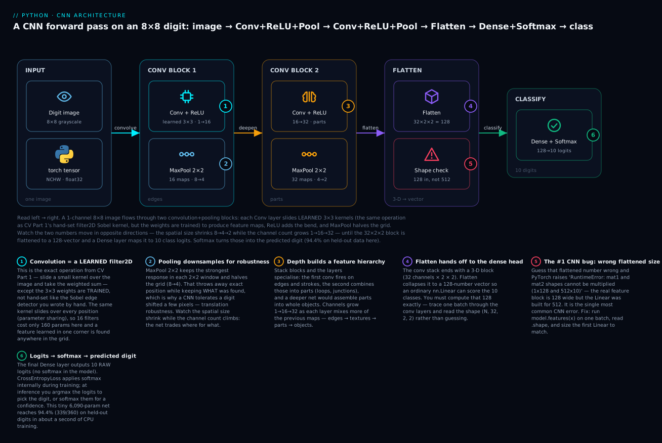
The six badges mark the teaching points in order: convolution as a learned filter2D (1), pooling for downsampling and robustness (2), depth building a feature hierarchy (3), the flatten hand-off (4), the flattened-size bug (5), and logits → softmax → class (6).
Building a CNN in PyTorch
Everything you learned about nn.Module in the PyTorch lesson carries over verbatim — declare layers in __init__, describe dataflow in forward, and the five-line loop trains it. The only new pieces are the conv and pool layers, and one bookkeeping chore that causes the single most common CNN bug: computing the size of the flattened feature block that feeds the first Linear.
Here is the model, built as two Conv → ReLU → Pool blocks (a features extractor) followed by a Flatten → Dropout → Linear head (a classifier), split deliberately so transfer learning later has a clean seam:
class DigitCNN(nn.Module):
    def __init__(self, classes=10, p_drop=0.25):
        super().__init__()                                # ALWAYS first
        self.features = nn.Sequential(
            nn.Conv2d(1, 16, kernel_size=3, padding=1),   # (N,1,8,8) -> (N,16,8,8)
            nn.ReLU(),
            nn.MaxPool2d(2),                              #           -> (N,16,4,4)
            nn.Conv2d(16, 32, kernel_size=3, padding=1),  #           -> (N,32,4,4)
            nn.ReLU(),
            nn.MaxPool2d(2),                              #           -> (N,32,2,2)
        )
        self.classifier = nn.Sequential(
            nn.Flatten(),                                 #           -> (N, 32*2*2 = 128)
            nn.Dropout(p_drop),
            nn.Linear(32 * 2 * 2, classes),               #           -> (N, 10) logits
        )
    def forward(self, x):
        x = self.features(x)
        return self.classifier(x)
The # => comments track the shape through every layer, and that column is not decoration — it is how you avoid the flattened-size bug. The first Linear must be told exactly how many numbers Flatten will hand it, and that number, 32 × 2 × 2 = 128, is the product of the final conv block’s output shape. Get it wrong and training dies before it starts (we detonate this deliberately in the lab). The bullet-proof way to find it is not arithmetic in your head — it is to run one batch through .features and read the shape:
torch.manual_seed(0)
model = DigitCNN()

with torch.no_grad():
    fmap = model.features(torch.zeros(1, 1, 8, 8))   # trace ONE dummy image
print(tuple(fmap.shape), "=> flatten to", fmap.numel())   # (1, 32, 2, 2) => flatten to 128
(1, 32, 2, 2) => flatten to 128
Now the parameter accounting, which makes the “few weights” story concrete. Each layer’s count, and the comparison to the equivalent MLP:
for name, mod in [("conv1", model.features[0]), ("conv2", model.features[3]),
                  ("linear", model.classifier[2])]:
    print(f"{name:7s}: {sum(p.numel() for p in mod.parameters()):5d} params")
print("TOTAL  :", sum(p.numel() for p in model.parameters()))

mlp = nn.Sequential(nn.Flatten(), nn.Linear(64, 32), nn.ReLU(), nn.Linear(32, 10))
print("MLP    :", sum(p.numel() for p in mlp.parameters()))
conv1  :   160 params
conv2  :  4640 params
linear :  1290 params
TOTAL  :  6090
MLP    :  2410
| Layer | Shape transform | Params | Why that many |
|---|---|---|---|
Conv2d(1, 16, 3) |
(1,8,8) → (16,8,8) | 160 | 16 filters × (1×3×3) + 16 biases |
MaxPool2d(2) |
(16,8,8) → (16,4,4) | 0 | Pooling has no weights |
Conv2d(16, 32, 3) |
(16,4,4) → (32,4,4) | 4,640 | 32 filters × (16×3×3) + 32 biases |
MaxPool2d(2) |
(32,4,4) → (32,2,2) | 0 | — |
Flatten |
(32,2,2) → (128,) | 0 | Just a reshape |
Linear(128, 10) |
(128,) → (10,) | 1,290 | 128×10 + 10 biases |
| Total | 6,090 |
Notice where the weights concentrate: the two conv layers together hold 160 + 4,640 = 4,800 params and do the actual seeing, while doing so at every spatial position through parameter sharing. On 8×8 images the CNN’s 6,090 is more than the MLP’s 2,410 — the small-image caveat from earlier, made real. Grow the image and the story inverts hard: the conv params stay fixed regardless of resolution, while the MLP’s first layer scales with the pixel count straight into the hundreds of millions.
Training the CNN, and watching it learn
The data pipeline is the digits dataset you met in the PyTorch lesson, with one difference that is the whole point: instead of flattening each image to a 64-vector, we keep it as an NCHW (1, 8, 8) grid so the convolutions can see the geometry.
import numpy as np
from torch.utils.data import TensorDataset, DataLoader
from sklearn.datasets import load_digits
from sklearn.model_selection import train_test_split

digits = load_digits()
X_img = digits.images                 # (1797, 8, 8) — the 2-D grids, NOT flattened
y = digits.target
print(X_img.shape, "range", X_img.min(), "-", X_img.max())   # (1797, 8, 8) range 0.0 - 16.0

X = X_img.reshape(-1, 1, 8, 8) / 16.0   # -> (N, 1, 8, 8) NCHW, scaled to 0..1
Xtr, Xte, ytr, yte = train_test_split(X, y, test_size=0.2, random_state=42, stratify=y)
Xtr = torch.tensor(Xtr, dtype=torch.float32);  ytr = torch.tensor(ytr, dtype=torch.long)
Xte = torch.tensor(Xte, dtype=torch.float32);  yte = torch.tensor(yte, dtype=torch.long)
print(tuple(Xtr.shape), Xtr.dtype)      # (1437, 1, 8, 8) torch.float32
(1797, 8, 8) range 0.0 - 16.0
(1437, 1, 8, 8) torch.float32
Two habits from the PyTorch lesson carry straight over and matter just as much here: features are float32, labels are int64 (long) because CrossEntropyLoss demands it, and we scaled pixels to [0, 1] (dividing by 16, the dataset’s max) so the inputs are normalised — an unnormalised image with values up to 16 makes early gradients large and training jumpy. From here the loop is identical to the MLP’s; only the model inside it changed:
train_dl = DataLoader(TensorDataset(Xtr, ytr), batch_size=64, shuffle=True)
criterion = nn.CrossEntropyLoss()                              # logits + long labels
optimizer = torch.optim.Adam(model.parameters(), lr=1e-3)      # the reliable default

def accuracy(m, Xd, yd):
    m.eval()
    with torch.no_grad():
        return (m(Xd).argmax(1) == yd).float().mean().item()

for epoch in range(1, 13):
    model.train()                                              # dropout ON
    running = 0.0
    for xb, yb in train_dl:
        optimizer.zero_grad()          # 1. clear old gradients (mandatory!)
        loss = criterion(model(xb), yb)  # 2+3. forward + loss
        loss.backward()                # 4. autograd fills every .grad
        optimizer.step()               # 5. update the 6,090 weights
        running += loss.item() * xb.size(0)
    if epoch == 1 or epoch % 3 == 0:
        print(f"epoch {epoch:2d} | loss {running/len(Xtr):.4f} "
              f"| train_acc {accuracy(model, Xtr, ytr):.3f} "
              f"| test_acc {accuracy(model, Xte, yte):.3f}")
Real output — the loss falls, the accuracy climbs, and it takes about a second on a CPU:
epoch  1 | loss 2.2723 | train_acc 0.537 | test_acc 0.536
epoch  3 | loss 1.9501 | train_acc 0.830 | test_acc 0.831
epoch  6 | loss 0.8045 | train_acc 0.905 | test_acc 0.875
epoch  9 | loss 0.4175 | train_acc 0.947 | test_acc 0.922
epoch 12 | loss 0.2817 | train_acc 0.958 | test_acc 0.944
print(f"FINAL test accuracy: {accuracy(model, Xte, yte):.4f} "
      f"({int(accuracy(model, Xte, yte)*len(yte))}/{len(yte)})")
# FINAL test accuracy: 0.9444 (339/360)
339 of 360 held-out digits classified correctly, by a 6,090-parameter network that learned its own edge detectors from scratch — no Sobel kernels written by hand. The train/test gap is small (0.958 vs 0.944), the healthy sign that it generalised rather than memorised. This is the same story the MLP told, but the CNN got there seeing the grid rather than a flattened row, which is why the same architecture scales to photographs where the MLP cannot follow.
| Epoch | Loss | Train acc | Test acc | Reading |
|---|---|---|---|---|
| 1 | 2.2723 | 0.537 | 0.536 | Just past random (10 classes = 10%) |
| 3 | 1.9501 | 0.830 | 0.831 | Edges learned, climbing fast |
| 6 | 0.8045 | 0.905 | 0.875 | Loss falling steeply |
| 9 | 0.4175 | 0.947 | 0.922 | Closing in |
| 12 | 0.2817 | 0.958 | 0.944 | Healthy small train–test gap |
Fighting overfitting: dropout, augmentation, batchnorm
A CNN with enough capacity will happily memorise the training set — training accuracy marching to 100% while held-out accuracy stalls or drops. That gap is overfitting, the central failure mode from the train/test lesson, and vision has three standard brakes. You already met dropout (it is in the model above); the two new ones are data augmentation and batch normalisation.
| Technique | How | What it does | Where it lives |
|---|---|---|---|
| Dropout | nn.Dropout(p) in the head |
Randomly zeroes activations so no neuron is load-bearing | Classifier head |
| Data augmentation | torchvision.transforms on inputs |
Randomly perturbs training images → more effective data | Data pipeline |
| Batch norm | nn.BatchNorm2d(C) after conv |
Normalises each channel per batch → stabler, faster training | Between conv and ReLU |
| Weight decay | Adam(..., weight_decay=1e-2) |
Penalises large weights → smoother function | Optimizer |
| Early stopping | Watch val loss, stop on rise | Halts before memorisation | Training loop |
Data augmentation: manufacture more images
The most effective vision-specific regulariser is data augmentation: apply random, label-preserving transformations to each training image — small rotations, shifts, crops, flips — so the network sees a slightly different picture every epoch and cannot memorise exact pixels. A cat rotated 8° or shifted 5 pixels is still a cat, so the label is unchanged while the input is fresh. torchvision.transforms composes these into a pipeline:
from torchvision import transforms

aug = transforms.Compose([
    transforms.RandomRotation(degrees=15),                 # tilt up to ±15°
    transforms.RandomAffine(degrees=0, translate=(0.12, 0.12)),  # shift up to 12%
])

one = Xtr[0:1]                        # one digit, shape (1, 1, 8, 8)
torch.manual_seed(3)
a1 = aug(one)                         # a random rotation
a2 = aug(one)                         # a different random shift
print("ink  orig:", round(one.sum().item(), 2),
      "| a1:", round(a1.sum().item(), 2), "| a2:", round(a2.sum().item(), 2))
print("pixels changed  a1:", int((a1 != one).sum()), "/64",
      "| a2:", int((a2 != one).sum()), "/64")
print("a1 == a2 ?", torch.equal(a1, a2))
ink  orig: 18.38 | a1: 14.69 | a2: 18.38
pixels changed  a1: 35 /64 | a2: 46 /64
a1 == a2 ? False
The same input produced two different images — one rotated (35 of 64 pixels changed), one shifted right by a column (46 changed) — and neither equals the original. Multiply that across every epoch and the network effectively trains on a far larger, more varied dataset without you collecting a single new sample. In practice you attach the transform to a Dataset so a fresh random version is drawn on every __getitem__, and — critically — you augment training data only, never validation or test (you evaluate on the real, un-perturbed images).
One honest, easily-missed caveat that the digits make vivid: augmentation must preserve the label, and which transforms do depends entirely on the data. A RandomHorizontalFlip is the canonical augmentation for natural photos (a mirror-image cat is still a cat) but is wrong for digits and text — a flipped 3 is not a 3, and a flipped 6 is not a 6. Rotating a digit 90° turns some digits into others. Choosing augmentations is a modelling decision about your data’s true invariances, not a checkbox.
| Transform | Call | Good for | Dangerous for |
|---|---|---|---|
| Horizontal flip | RandomHorizontalFlip() |
Natural photos (cats, cars) | Digits, text, signs (changes meaning) |
| Small rotation | RandomRotation(15) |
Most images | Large angles that confuse classes |
| Random crop/resize | RandomResizedCrop(224) |
The ImageNet standard | Tiny objects that crop out |
| Translate/shift | RandomAffine(0, translate=...) |
Robustness to position | — |
| Colour jitter | ColorJitter(...) |
Lighting robustness | Tasks where colour is the label |
| Normalize | Normalize(mean, std) |
Always (match the model) | Wrong mean/std hurts pretrained nets |
Batch normalisation: stabilise the activations
Batch normalisation (nn.BatchNorm2d) inserts a step after a conv layer that normalises each channel to roughly zero-mean, unit-variance using the current batch’s statistics, then rescales with two learned parameters. It makes deep networks train faster and more stably, and it has a mild regularising effect. But it carries the same train()/eval() hazard as dropout — and a subtler one, because in training it uses the batch’s own statistics while in eval it uses running statistics accumulated during training. Forget model.eval() at inference and batchnorm silently uses the wrong statistics. You can watch the two modes diverge:
bn = nn.BatchNorm2d(3)
train_batch = torch.randn(16, 3, 4, 4) + 5.0   # data centred around +5
bn.train()
for _ in range(20):
    bn(train_batch)                              # accumulate running stats toward ~5
print("running_mean learned:", [round(v, 2) for v in bn.running_mean.tolist()])

new_batch = torch.randn(16, 3, 4, 4) + 0.0       # a NEW batch centred around 0
bn.train(); print("train-mode output mean:", round(bn(new_batch).mean().item(), 3))
bn.eval();  print("eval-mode  output mean:", round(bn(new_batch).mean().item(), 3))
running_mean learned: [4.43, 4.5, 4.41]
train-mode output mean: 0.0
eval-mode  output mean: -3.892
In train() mode batchnorm re-centres the new batch using its own mean, so the output mean is 0.0. In eval() mode it subtracts the stored running mean (~4.5, learned from the +5 training data), so the same zero-centred batch comes out at -3.892. Neither is a bug — it is the design — but it means the mode flag changes your numbers, and using train() at inference (or forgetting to let running stats warm up) gives quietly wrong predictions. As with dropout: model.eval() before you evaluate, always.
Transfer learning: standing on a pretrained backbone
Here is the most important practical truth in applied computer vision: you almost never train a CNN from scratch. Training a competitive image model needs millions of labelled images and days of GPU time — resources you rarely have. Instead you take a network already trained on a giant dataset (ImageNet: 1.2 million images, 1000 classes), keep its learned backbone (which already knows edges, textures, and object parts — features that transfer to almost any vision task), and retrain only a small new head for your classes. This is transfer learning, and it is how essentially all real image classifiers are built.
The recipe has three moves, and torchvision hands you the pretrained model in one line. We load a real ResNet-18 (a classic 18-layer residual CNN) with its ImageNet weights:
from torchvision.models import resnet18, ResNet18_Weights

weights = ResNet18_Weights.DEFAULT
backbone = resnet18(weights=weights)        # downloads once, then cached (~45 MB)
print("total params:", sum(p.numel() for p in backbone.parameters()))   # 11,689,512
print("first conv:", backbone.conv1)
print("first filter bank:", tuple(backbone.conv1.weight.shape))   # (64, 3, 7, 7)
print("original head:", backbone.fc)        # Linear(in_features=512, out_features=1000)
total params: 11689512
first conv: Conv2d(3, 64, kernel_size=(7, 7), stride=(2, 2), padding=(3, 3), bias=False)
first filter bank: (64, 3, 7, 7)
original head: Linear(in_features=512, out_features=1000, bias=True)
That first layer — (64, 3, 7, 7) — is 64 learned filters, each 7×7 over the 3 colour channels: the trained equivalents of your hand-written Sobel kernel, and if you visualise them they look like oriented edge and colour-blob detectors, exactly the hierarchy’s first rung. Now the three transfer-learning moves: freeze the backbone so its learned features are preserved, replace the 1000-class ImageNet head with a fresh head for your number of classes, and train only the head:
# 1. FREEZE the backbone — no gradients, its features are already good
for p in backbone.parameters():
    p.requires_grad = False

# 2. REPLACE the head — a fresh Linear for 10 classes (new params train by default)
in_feat = backbone.fc.in_features            # 512
backbone.fc = nn.Linear(in_feat, 10)

# 3. count what will actually train
trainable = sum(p.numel() for p in backbone.parameters() if p.requires_grad)
frozen    = sum(p.numel() for p in backbone.parameters() if not p.requires_grad)
print(f"trainable: {trainable} (just the head) | frozen: {frozen}")
trainable: 5130 (just the head) | frozen: 11176512
You would now train that model with the same five-line loop, and the optimizer only touches the 5,130 head parameters — the other 11,176,512 are frozen — so it converges in a handful of epochs on a few hundred images, no GPU required. (We do not run that loop here: ResNet expects 224×224 three-channel photos, and upscaling 8×8 gray digits to feed it is a contrived exercise. The setup is the transferable skill, and it is real.) One non-negotiable detail: a pretrained model demands the exact preprocessing it was trained with — the same resize, crop, and channel normalisation — or its features misfire. torchvision ships those with the weights:
print(weights.transforms())
ImageClassification(
    crop_size=[224]
    resize_size=[256]
    mean=[0.485, 0.456, 0.406]
    std=[0.229, 0.224, 0.225]
    interpolation=InterpolationMode.BILINEAR
)
Those mean/std triples are the ImageNet channel statistics; feed a pretrained ResNet images normalised any other way and accuracy quietly craters. Always apply weights.transforms() (or replicate it exactly). The two transfer-learning strategies, and when to pick each:
| Strategy | What trains | Use when | Speed |
|---|---|---|---|
| Feature extraction (freeze) | Only the new head | Small dataset, classes similar to ImageNet | Fastest — head is tiny |
| Fine-tuning | Head + some/all backbone (low LR) | More data, or a domain far from ImageNet | Slower, needs a GPU |
| From scratch | Everything | You have millions of images + compute | Slowest — rarely the right call |
The rule of thumb: start frozen. Train just the head; if that plateaus below what you need and you have enough data, unfreeze the top backbone blocks and fine-tune with a small learning rate (e.g. 1e-4, ten times lower, so you nudge the pretrained weights rather than wreck them). Training a whole ResNet from random weights is the last resort, reserved for when your data is both huge and utterly unlike natural photos.
torchvision ships dozens of pretrained backbones behind the identical one-line API; these are the ones worth knowing, with their real parameter counts (measured on torchvision 0.28):
| Backbone | torchvision.models |
Params | Reach for it when |
|---|---|---|---|
| ResNet-18 | resnet18 |
11,689,512 | Default starter — small, fast, strong |
| ResNet-50 | resnet50 |
25,557,032 | More accuracy when you have the compute |
| MobileNet-V3-Small | mobilenet_v3_small |
2,542,856 | Phones / edge / real-time — tiny and quick |
| EfficientNet-B0 | efficientnet_b0 |
5,288,548 | Best accuracy-per-parameter in a small net |
| ViT-B/16 | vit_b_16 |
86,567,656 | Large datasets where a transformer beats a CNN |
The pattern is always the same regardless of which you pick: load with weights=...DEFAULT, freeze, swap the final layer (.fc on ResNet, .classifier[-1] on MobileNet/EfficientNet, .heads.head on ViT), and train. Start with ResNet-18 — it is the sensible default and what most tutorials assume.
The same CNN in Keras (for comparison)
For completeness, the identical two-block CNN in Keras — shown for structural comparison and, honestly, not executed here (this lesson does not install TensorFlow; the PyTorch/Keras lesson executes the Keras side of an equivalent MLP). Keras hides the training loop behind compile/fit, and it uses NHWC ordering (channels last, (8, 8, 1)) — the opposite of PyTorch’s NCHW, a frequent porting bug:
# NOT executed in this lesson — shown for comparison (needs: pip install tensorflow)
from tensorflow import keras
from keras import layers

model = keras.Sequential([
    keras.Input(shape=(8, 8, 1)),                          # NHWC: channels LAST
    layers.Conv2D(16, 3, padding="same", activation="relu"),
    layers.MaxPooling2D(2),
    layers.Conv2D(32, 3, padding="same", activation="relu"),
    layers.MaxPooling2D(2),
    layers.Flatten(),
    layers.Dropout(0.25),
    layers.Dense(10),                                      # logits, like PyTorch
])
model.compile(optimizer=keras.optimizers.Adam(1e-3),
              loss=keras.losses.SparseCategoricalCrossentropy(from_logits=True),
              metrics=["accuracy"])
model.fit(X_train, y_train, epochs=12, batch_size=64)      # the loop, hidden
Same architecture, same 10-logit output, same Adam and cross-entropy — the difference is that Keras’s fit owns the loop while PyTorch makes you write it. The one thing to watch when moving between them is the channel-axis convention: PyTorch (N, 1, 8, 8) versus Keras (N, 8, 8, 1). Feed a Keras model NCHW data and it will either error or silently treat height as channels.
Object detection basics: from “what” to “what and where”
Classifying a whole image — “this is a 7” — is only the simplest vision task. Real scenes contain many objects, and you often need to know what each one is and where it sits. This is a different problem with a different output, and while training a detector is beyond a CPU lesson, the concepts are essential vocabulary. Start by separating the three tasks people conflate:
| Task | Question answered | Output | Example |
|---|---|---|---|
| Classification | What is this image? | One class label (+ probability) | “This image is a cat” |
| Classification + localisation | What, and where (one object)? | One label + one bounding box | “A cat, in this box” |
| Object detection | What and where, for every object? | A list of (box, class, score) | “3 cats and 2 dogs, boxed” |
| Semantic segmentation | Which class is each pixel? | A per-pixel class map | Every pixel labelled cat/dog/bg |
| Instance segmentation | Which object owns each pixel? | Per-pixel + per-instance masks | Cat #1 vs cat #2, pixel-exact |
Object detection outputs, per object, a bounding box (four numbers — typically [x1, y1, x2, y2]), a class, and a confidence score. Under the hood it is still a CNN backbone extracting features; the difference is the head, which must propose regions and classify each. Two architectural families dominate, and the trade-off between them is the classic speed/accuracy dial:
| Family | Examples | How it works | Trade-off |
|---|---|---|---|
| Two-stage | Faster R-CNN, Mask R-CNN | 1) propose candidate regions, 2) classify + refine each | More accurate, slower |
| One-stage | YOLO, SSD, RetinaNet | Predict boxes + classes in a single pass over a grid | Faster (real-time), historically a touch less accurate |
The intuition: a two-stage detector like Faster R-CNN first asks “where might objects be?” (a region-proposal network) and then “what is in each proposed box?” — two passes, higher accuracy, more compute. A one-stage detector like YOLO (“You Only Look Once”) skips the proposal step and predicts every box and class in one sweep of the image, which is what makes YOLO fast enough for real-time video. Modern versions of both are excellent; you pick based on whether you need maximum accuracy (two-stage) or real-time speed (one-stage).
The two metrics: IoU and mAP
Detection needs metrics that score boxes, not just labels, and both rest on Intersection over Union (IoU) — the overlap between a predicted box and the ground-truth box, divided by their combined area. IoU ranges 0 (no overlap) to 1 (perfect), and it is pure geometry you can compute by hand; torchvision agrees:
from torchvision.ops import box_iou

pred = torch.tensor([[10., 10., 50., 50.]])   # a 40x40 predicted box, area 1600
gt   = torch.tensor([[30., 30., 70., 70.]])   # a 40x40 truth box,     area 1600
# overlap is x∈[30,50], y∈[30,50] = 20x20 = 400 ; union = 1600+1600-400 = 2800
print("manual IoU:", round(400 / 2800, 4))    # 0.1429
print("box_iou   :", round(box_iou(pred, gt).item(), 4))   # 0.1429
manual IoU: 0.1429
box_iou   : 0.1429
A prediction usually counts as correct if its IoU with a true box clears a threshold (commonly 0.5). Detectors also emit many overlapping boxes for the same object, so a step called Non-Max Suppression (NMS) keeps the highest-scoring box and drops its heavy-overlap duplicates:
from torchvision.ops import nms
boxes  = torch.tensor([[10.,10.,50.,50.], [12.,12.,52.,52.], [100.,100.,140.,140.]])
scores = torch.tensor([0.9, 0.8, 0.75])
print("NMS keeps:", nms(boxes, scores, iou_threshold=0.5).tolist())   # [0, 2]
NMS keeps: [0, 2]
NMS kept box 0 (score 0.9) and box 2 (a separate object), and dropped box 1 — a 0.8-scoring near-duplicate of box 0. The headline detection metric is mAP (mean Average Precision): for each class you sweep the confidence threshold to trace a precision–recall curve (the precision/recall ideas from the metrics lesson, applied to IoU-matched boxes), take the area under it (Average Precision), and average across classes. “mAP@0.5” uses an IoU cutoff of 0.5; “mAP@[.5:.95]” averages over many cutoffs and is the strict COCO standard. Higher is better; it is the number every detection paper reports.
| Metric | Measures | Range | Note |
|---|---|---|---|
| IoU | Overlap of two boxes | 0–1 | The atom of every detection metric |
| NMS | (a step, not a metric) | — | Removes duplicate boxes for one object |
| Precision / Recall | Correct vs missed detections | 0–1 | A box is “correct” if IoU ≥ threshold |
| AP | Area under one class’s PR curve | 0–1 | Per-class summary |
| mAP | Mean AP over all classes | 0–1 | The headline detection score |
Using a detector, and where the field is going
In practice you use a pretrained detector rather than train one. torchvision ships them with the same one-line API as the classifier — fasterrcnn_resnet50_fpn(weights=...) loads a Faster R-CNN pretrained on COCO (80 everyday classes), and calling it on an image returns a list of dicts with boxes, labels, and scores tensors; you filter by score, apply NMS, and draw the boxes. (We describe rather than run it here — the weights are a ~160 MB download and CPU inference is slow, but the API mirrors the ResNet load above exactly.) For anything custom you would fine-tune such a detector, or reach for the Ultralytics YOLO library, which wraps training and inference into a few lines.
Two honest limits to close on. First, CNNs are hungry — they need substantial labelled data and, to train from scratch, real compute; transfer learning is what makes them practical, and it is why this lesson spends more time on using pretrained models than training them. Second, the CNN’s decade of dominance is no longer absolute: Vision Transformers (ViT) — which apply the attention mechanism behind large language models to image patches instead of convolutions — now match or beat CNNs on large datasets, and modern systems increasingly blend the two. CNNs remain the right first tool (they are more data-efficient on small datasets, faster on modest hardware, and the concepts here transfer directly), but “convolution is the only way to do vision” stopped being true around 2021. The architecture map from the PyTorch lesson still holds: pick the architecture that matches your data’s structure, and for images that is a CNN today and, increasingly, a transformer tomorrow.
To close the two computer-vision lessons, here is when to reach for each of the three approaches you now know — the hand-tuned pipeline from CV Part 1, the CNN from this lesson, and the transformer on the horizon:
| Approach | Best when | Data need | Compute | Interpretable? |
|---|---|---|---|---|
| Classical CV (CV Part 1) | Well-defined geometric tasks (barcodes, well-lit shapes) | None | Runs on a Raspberry Pi | High — every step explicit |
| CNN (this lesson) | Most image tasks; small–medium datasets | Hundreds–thousands (with transfer) | CPU inference; GPU to train from scratch | Low — but visualisable filters |
| Vision Transformer | Very large datasets, top accuracy | Millions (or a huge pretrain) | GPU-heavy | Low |
The honest default for a working engineer: use classical CV for the plumbing (load, denoise, crop, colour-normalise), a pretrained CNN via transfer learning for the perception, and only investigate a ViT when you have the data and compute to justify it.
Hands-on lab: a CNN digit classifier, start to finish
⏱️ ~10 minutes, entirely on CPU. You will build the two-block CNN, train it, watch loss fall and accuracy rise, evaluate on held-out data, break it on purpose with the flattened-size bug, apply a data-augmentation transform, and load a real pretrained ResNet to set up transfer learning. Everything runs offline — the digits ship inside scikit-learn.
⚠️ The only network access is the first resnet18(weights=...) call (step 7), which downloads ~45 MB once and then caches. If you are fully offline, skip step 7; steps 1–6 need no network.
Step 0 — Environment
python3 -m venv .venv
source .venv/bin/activate                 # Windows: .venv\Scripts\activate
python -m pip install --upgrade pip

pip install scikit-learn                   # bundles the 8x8 digits (no download)
# PyTorch + torchvision, CPU-only build (all this lesson needs)
pip install torch torchvision --index-url https://download.pytorch.org/whl/cpu

python -c "import torch, torchvision; print(torch.__version__, torchvision.__version__)"
# => 2.13.0 0.28.0
Step 1 — Data as NCHW grids (not flattened)
import numpy as np, torch, torch.nn as nn
from torch.utils.data import TensorDataset, DataLoader
from sklearn.datasets import load_digits
from sklearn.model_selection import train_test_split

torch.manual_seed(0)
digits = load_digits()
X = digits.images.reshape(-1, 1, 8, 8) / 16.0             # (N,1,8,8) NCHW, 0..1
y = digits.target
Xtr, Xte, ytr, yte = train_test_split(X, y, test_size=0.2, random_state=42, stratify=y)
Xtr = torch.tensor(Xtr, dtype=torch.float32); ytr = torch.tensor(ytr, dtype=torch.long)
Xte = torch.tensor(Xte, dtype=torch.float32); yte = torch.tensor(yte, dtype=torch.long)
train_dl = DataLoader(TensorDataset(Xtr, ytr), batch_size=64, shuffle=True)
print(tuple(Xtr.shape), "| batches/epoch:", len(train_dl))   # (1437, 1, 8, 8) | 23
What just happened: the images stay as (1, 8, 8) grids so convolutions can see the geometry — the one change from the MLP lab. Features float32, labels long, pixels scaled to [0, 1].
Step 2 — Define the CNN and verify the flattened size
class DigitCNN(nn.Module):
    def __init__(self, classes=10, p_drop=0.25):
        super().__init__()
        self.features = nn.Sequential(
            nn.Conv2d(1, 16, 3, padding=1), nn.ReLU(), nn.MaxPool2d(2),
            nn.Conv2d(16, 32, 3, padding=1), nn.ReLU(), nn.MaxPool2d(2))
        self.classifier = nn.Sequential(
            nn.Flatten(), nn.Dropout(p_drop), nn.Linear(32 * 2 * 2, classes))
    def forward(self, x):
        return self.classifier(self.features(x))

model = DigitCNN()
print(model.features(Xtr[:1]).shape, "-> flatten", model.features(Xtr[:1]).numel())
# torch.Size([1, 32, 2, 2]) -> flatten 128
print("params:", sum(p.numel() for p in model.parameters()))   # 6090
What just happened: tracing one image through .features confirms the (1, 32, 2, 2) block flattens to 128 — the number the first Linear must expect. Always verify this rather than guess.
Step 3 — Train (watch it learn)
criterion = nn.CrossEntropyLoss()
optimizer = torch.optim.Adam(model.parameters(), lr=1e-3)

def acc(m, X, y):
    m.eval()
    with torch.no_grad(): return (m(X).argmax(1) == y).float().mean().item()

for epoch in range(1, 13):
    model.train()
    for xb, yb in train_dl:
        optimizer.zero_grad()
        loss = criterion(model(xb), yb)
        loss.backward()
        optimizer.step()
    if epoch % 3 == 0:
        print(f"epoch {epoch:2d} | test_acc {acc(model, Xte, yte):.3f}")
epoch  3 | test_acc 0.831
epoch  6 | test_acc 0.875
epoch  9 | test_acc 0.922
epoch 12 | test_acc 0.944
What just happened: the same five-line loop as the MLP, now driving a CNN — test accuracy climbs to 94.4% in about a second on CPU.
Step 4 — Evaluate correctly
model.eval()
with torch.no_grad():
    preds = model(Xte).argmax(1)
correct = (preds == yte).sum().item()
print(f"FINAL: {correct}/{len(yte)} = {correct/len(yte):.4f}")   # 339/360 = 0.9444
What just happened: 339 of 360 held-out digits correct. eval() + no_grad() is the inference idiom — dropout off, no graph built.
Step 5 — Break it on purpose: the flattened-size bug
class BrokenCNN(nn.Module):
    def __init__(self):
        super().__init__()
        self.features = nn.Sequential(
            nn.Conv2d(1, 16, 3, padding=1), nn.ReLU(), nn.MaxPool2d(2),
            nn.Conv2d(16, 32, 3, padding=1), nn.ReLU(), nn.MaxPool2d(2))
        self.classifier = nn.Sequential(
            nn.Flatten(), nn.Linear(32 * 4 * 4, 10))   # WRONG: guessed 4x4, real is 2x2
    def forward(self, x):
        return self.classifier(self.features(x))

try:
    BrokenCNN()(Xtr[:1])
except RuntimeError as e:
    print("RuntimeError:", e)
RuntimeError: mat1 and mat2 shapes cannot be multiplied (1x128 and 512x10)
What just happened: guessing the flattened size as 32×4×4=512 instead of the real 32×2×2=128 produces the most common CNN error there is. The real feature block is 1×128; the Linear was built for 512 inputs. The message even tells you both numbers — (1x128 and 512x10).
Step 6 — Data augmentation
from torchvision import transforms
aug = transforms.Compose([transforms.RandomRotation(15),
                          transforms.RandomAffine(0, translate=(0.12, 0.12))])
torch.manual_seed(3)
a1, a2 = aug(Xtr[0:1]), aug(Xtr[0:1])
print("pixels changed:", int((a1 != Xtr[0:1]).sum()), "and", int((a2 != Xtr[0:1]).sum()),
      "| identical?", torch.equal(a1, a2))
# pixels changed: 35 and 46 | identical? False
What just happened: one image yielded two different augmented versions — a rotation and a shift — so the network sees fresh data every epoch. (Augment train only; never flip digits — a mirrored 3 is not a 3.)
Step 7 — Set up transfer learning on a pretrained ResNet
from torchvision.models import resnet18, ResNet18_Weights
backbone = resnet18(weights=ResNet18_Weights.DEFAULT)   # downloads once, then cached
for p in backbone.parameters():                          # freeze the backbone
    p.requires_grad = False
backbone.fc = nn.Linear(backbone.fc.in_features, 10)     # fresh 10-class head
trainable = sum(p.numel() for p in backbone.parameters() if p.requires_grad)
print("first-layer filters:", tuple(backbone.conv1.weight.shape))  # (64, 3, 7, 7)
print("trainable now:", trainable, "of", sum(p.numel() for p in backbone.parameters()))
# trainable now: 5130 of 11181642
What just happened: a real 11.7M-parameter ImageNet model, its backbone frozen, its head swapped for your 10 classes — now only 5,130 parameters would train. This is how production image classifiers are actually built.
Common mistakes and troubleshooting
Every row is a real traceback or behaviour captured on PyTorch 2.13. These are the CNN-specific errors on top of the general PyTorch ones from the previous lesson.
| Symptom / traceback | Cause | Fix |
|---|---|---|
RuntimeError: mat1 and mat2 shapes cannot be multiplied (1x128 and 512x10) |
The #1 CNN bug — wrong flattened size into the first Linear |
Run model.features(x) on one batch, read .shape, size Linear to C×H×W |
RuntimeError: Given groups=1, ... expected input [N, 1, H, W] to have 3 channels, but got 1 |
Wrong in_channels — gray image into a 3-channel conv |
Match Conv2d(in_channels=...) to the image (1 gray, 3 colour) |
RuntimeError: expected input ... 4-dimensional ... but got ... [N, H, W] |
Missing channel axis (fed (N, 8, 8)) |
Reshape to NCHW: x.reshape(-1, 1, 8, 8) or x.unsqueeze(1) |
| Colours look wrong / accuracy poor with OpenCV images | NHWC (or BGR) fed to a NCHW model |
img[..., ::-1] for BGR→RGB, then .permute(2,0,1) for HWC→CHW |
| Loss stuck ~2.3 (=ln 10), never falls | Inputs not normalised (pixels 0–255 or 0–16) | Scale to [0,1] (/255 or /16) or standardise |
RuntimeError: expected scalar type Long but found Float |
Float labels into CrossEntropyLoss |
Labels must be long integer class indices |
Loss becomes nan after a few steps |
Learning rate too high | Drop lr 10× (try 1e-3); check for unscaled inputs |
| Pretrained model far less accurate than expected | Wrong preprocessing (skipped ImageNet mean/std) | Apply weights.transforms() — same resize/crop/normalize as training |
| Predictions randomly worse than training suggested | Forgot model.eval() — dropout/batchnorm still in train mode |
model.eval() (and torch.no_grad()) before inference |
| Train acc → 1.0, test acc stuck/dropping | Overfitting | Add dropout / augmentation; get more data; early-stop |
| Training crawls / “CPU is too slow” on a big net | Training a large CNN from scratch on CPU | Use a small net, or a frozen pretrained backbone (trains the tiny head only) |
Three gotchas earn extra words because they cost the most time.
The flattened-size mismatch is the CNN rite of passage. The conv/pool stack outputs a 3-D block (channels, height, width), and Flatten turns it into a vector of channels × height × width numbers that the first Linear must be built to accept. Miscount — forget a pooling step halves the size, or assume the wrong final resolution — and you get mat1 and mat2 shapes cannot be multiplied, with the two mismatched numbers right there in the message (1x128 and 512x10 means “I have 128 features but you built the layer for 512”). Never compute this by hand under pressure: run one batch through .features, print .shape, done. Some people sidestep it entirely with nn.AdaptiveAvgPool2d(1) before the head, which forces a fixed size regardless of input resolution.
Channel order and count are two different traps, both silent-ish. NCHW versus NHWC (PyTorch vs Keras/TensorFlow, and vs the (H,W,C) you get from OpenCV/Pillow) will either error loudly about dimensions or, worse, run with height misread as channels and give nonsense. Separately, an in_channels mismatch — a 1-channel grayscale image into a conv expecting 3, or vice versa — raises the “expected 3 channels, but got 1” error. The fix for OpenCV images is the two-step img[..., ::-1] (BGR→RGB from CV Part 1) then torch.from_numpy(img).permute(2, 0, 1).unsqueeze(0) (HWC→CHW, add batch).
Forgetting to normalise inputs quietly caps your accuracy. A CNN fed raw pixels (0–255, or the digits’ 0–16) sees large, uneven inputs that make early gradients unstable; the loss often parks near ln(10) ≈ 2.30 (random guessing for 10 classes) and barely moves. Scaling to [0, 1] or standardising fixes it. For a pretrained model the requirement is stricter still: you must use the exact ImageNet mean/std the model trained with, delivered by weights.transforms() — any other normalisation silently degrades its features.
Cheat-sheet
| Task | Code |
|---|---|
| Conv layer | nn.Conv2d(in_ch, out_ch, kernel_size=3, padding=1) |
| Kernel weight shape | (out_channels, in_channels, kH, kW) |
| Image tensor shape | NCHW = (batch, channels, height, width) |
| Max / avg pool | nn.MaxPool2d(2) · nn.AvgPool2d(2) |
| “Same” padding (3×3) | padding=1 (keeps H×W); padding=0 = “valid” (shrinks) |
| Output size formula | out = (in + 2·pad − k) / stride + 1 |
| Flatten for the head | nn.Flatten() → vector of C×H×W |
| Find the flattened size | model.features(x).shape on one batch — never guess |
| Batch norm | nn.BatchNorm2d(channels) after conv |
| Dropout | nn.Dropout(p) in the head |
| Feature extractor + head | self.features = Sequential(...); self.classifier = Sequential(...) |
| Loss (classify) | nn.CrossEntropyLoss() — logits + long labels |
| Data augmentation | transforms.Compose([RandomRotation(15), RandomAffine(...)]) |
| Load pretrained model | resnet18(weights=ResNet18_Weights.DEFAULT) |
| Its required preprocessing | weights.transforms() (ImageNet mean/std) |
| Freeze the backbone | for p in model.parameters(): p.requires_grad = False |
| Replace the head | model.fc = nn.Linear(model.fc.in_features, n_classes) |
| HWC (OpenCV) → NCHW | torch.from_numpy(img).permute(2,0,1).unsqueeze(0) |
| BGR → RGB (CV Part 1) | img[..., ::-1] |
| IoU of boxes | torchvision.ops.box_iou(a, b) |
| Non-max suppression | torchvision.ops.nms(boxes, scores, iou_threshold) |
| Pretrained detector | torchvision.models.detection.fasterrcnn_resnet50_fpn(weights=...) |
Interview and exam questions
Q: Why does a fully-connected MLP struggle on real images, and how does a convolution fix it? A: Three reasons. Flattening discards spatial structure (which pixels were neighbours); every-input-to-every-neuron wiring causes a parameter explosion (a 224×224×3 image into 1000 hidden units is ~150 million weights in one layer); and it has no translation invariance (a shifted object lands on unrelated inputs). A convolution fixes all three via local connectivity (each output sees a small patch, geometry preserved) and parameter sharing (one small kernel slides everywhere, so the param count is independent of image size — 1,792 for 64 filters — and a feature is detected wherever it appears).
Q: In one sentence, how does a CNN relate to cv2.filter2D from classical computer vision?
A: A convolution is the same sliding-weighted-sum operation as filter2D, except the kernel weights are learned by gradient descent instead of hand-designed — the network discovers its own edge/texture/part detectors rather than you writing a Sobel kernel.
Q: What do stride and padding control, and what are “same” vs “valid” convolution?
A: stride is the step size as the kernel slides (>1 downsamples the output); padding adds a border of zeros before sliding. “Valid” = no padding, so the output shrinks by (k−1) (an 8×8 → 6×6 with a 3×3 kernel). “Same” = padding=(k−1)/2, which keeps the output the same size as the input — the common default, since you then control downsampling deliberately with pooling.
Q: What does pooling do, and why does it help? A: Pooling downsamples a feature map by summarising each window into one number (usually the max). It shrinks the data (cheaper deeper layers) and adds translation robustness — the max of a 2×2 window rarely changes when the input shifts a pixel, so the network tolerates small position changes.
Q: You build a CNN and get RuntimeError: mat1 and mat2 shapes cannot be multiplied (1x128 and 512x10). What happened and how do you fix it?
A: The flattened-size bug — the #1 CNN error. The conv/pool stack produced a feature block that flattens to 128 numbers, but the first Linear was built for 512 inputs. Fix: run model.features(x) on one batch, read the (C, H, W) shape, and set the Linear to C×H×W (here 32×2×2 = 128). Don’t compute it by hand — trace one batch.
Q: What is NCHW, and why does it matter when moving code between PyTorch, Keras, and OpenCV?
A: NCHW = (batch, channels, height, width), PyTorch’s tensor layout with the channel axis second. Keras/TensorFlow use NHWC (channels last), and OpenCV/Pillow give you (H, W, C). Feeding the wrong layout either errors about dimensions or silently misreads height as channels. Convert OpenCV images with .permute(2, 0, 1).unsqueeze(0) (and fix BGR→RGB first).
Q: What is transfer learning, and why is it the norm rather than training from scratch? A: Take a network pretrained on a huge dataset (ImageNet), keep its backbone (which already learned edges/textures/parts that transfer to most vision tasks), and retrain only a new head for your classes. It is the norm because training a competitive CNN from scratch needs millions of labelled images and heavy GPU time; transfer learning reaches strong accuracy from a few hundred images in minutes. Start by freezing the backbone and training just the head; fine-tune deeper layers with a low LR only if needed.
Q: A colleague loads a pretrained ResNet, feeds it images scaled to [0,1], and accuracy is terrible. Why?
A: Wrong preprocessing. A pretrained model must receive images normalised exactly as it was trained — for ImageNet models that means the specific per-channel mean=[0.485,0.456,0.406]/std=[0.229,0.224,0.225] plus the right resize/crop, delivered by weights.transforms(). Any other normalisation shifts the inputs off the distribution the frozen features expect, and accuracy craters.
Q: Distinguish classification, object detection, and segmentation. A: Classification gives one label for the whole image (“a cat”). Object detection gives a list of (bounding box, class, score) for every object (“3 cats and 2 dogs, each boxed”). Segmentation labels every pixel — semantic segmentation by class, instance segmentation by individual object. They differ in output shape and difficulty, but all use a CNN (or transformer) backbone.
Q: What are IoU and mAP? A: IoU (Intersection over Union) measures box overlap — the area of intersection divided by the area of union of a predicted and a true box (0 = no overlap, 1 = perfect); a detection counts as correct if IoU clears a threshold (often 0.5). mAP (mean Average Precision) is the headline detection metric: the area under each class’s precision–recall curve (Average Precision), averaged over classes; “mAP@0.5” uses IoU 0.5, “mAP@[.5:.95]” averages over stricter cutoffs.
Q: One-stage vs two-stage detectors — what’s the trade-off? A: Two-stage (Faster R-CNN): first propose candidate regions, then classify and refine each — more accurate, slower. One-stage (YOLO, SSD): predict all boxes and classes in a single pass over the image — faster, real-time capable, historically a touch less accurate. Pick by whether you need maximum accuracy or real-time speed.
Q (coding): Given an OpenCV BGR image array img of shape (H, W, 3), turn it into a batch-of-one tensor a PyTorch CNN can accept.
A:
rgb = img[..., ::-1].copy()                      # BGR -> RGB (CV Part 1)
t = torch.from_numpy(rgb).permute(2, 0, 1)       # HWC -> CHW
t = t.float().unsqueeze(0) / 255.0               # add batch axis, scale to [0,1] -> (1,3,H,W)
Key takeaways
- A CNN is
filter2Dwith learned kernels. The convolution is the exact sliding-weighted-sum from CV Part 1; the network learns the weights by the same five-line training loop from the PyTorch lesson. We proved it by loading a hand-set Sobel kernel into annn.Conv2dand getting the same edge response (±36). - A plain MLP fails on images three ways — it discards spatial structure, explodes to ~150M parameters on a real photo, and lacks translation invariance. Convolution fixes all three through local connectivity and parameter sharing (1,792 params for 64 filters, independent of image size).
- The classic architecture is
[Conv → ReLU → Pool] × N → Flatten → Dense → logits: spatial size shrinks, channels grow, and depth builds a hierarchy (edges → textures → parts → objects). The conv stack is the backbone; the dense layers are the head. - The #1 CNN bug is the flattened-size mismatch (
mat1 and mat2 shapes cannot be multiplied). Never guess it — runmodel.features(x)on one batch and read the shape. Our net’s(32,2,2)block flattens to128. - Our 6,090-param CNN hit 94.4% (339/360) on held-out digits in ~1 second of CPU training. Fight overfitting with dropout, data augmentation (label-preserving — never flip digits), and batch normalisation (which, like dropout, behaves differently in
train()vseval()). - You rarely train from scratch. Transfer learning loads a pretrained backbone (real ResNet-18: 11.7M params), freezes it, and retrains a tiny head (5,130 params) — and demands the model’s exact preprocessing (
weights.transforms()). - Object detection adds where to what: per-object (box, class, score), scored by IoU and mAP, cleaned with NMS, built as one-stage (YOLO, fast) or two-stage (Faster R-CNN, accurate) detectors. You use pretrained detectors far more than you train them — and Vision Transformers are now a serious alternative to CNNs on large data.