Everything a language model, a search engine, a spam filter, or a sentiment classifier does begins with the same awkward fact: a model does arithmetic, and text is not numbers. You cannot subtract “Tuesday” from “cat” or feed the string "not good" into a matrix multiply. Before any learning happens, raw text has to be turned into rows of numbers — and the quality of that transformation decides the ceiling of everything downstream. Garbage tokens in, garbage predictions out.
Natural Language Processing (NLP) is the discipline of doing that transformation well, and this lesson is the foundation: the preprocessing pipeline that turns messy human text into a clean numeric feature matrix. We will tokenize (split text into units), normalize (collapse the thousand surface forms of a word into one), and vectorize (count those units into numbers), using the two libraries every Python practitioner meets — NLTK, the teaching toolkit, and spaCy, the production pipeline — and scikit-learn’s vectorizers to reach the numbers.
This is Part 1 of 2. Part 2 picks up where the feature matrix ends — text classification and the contextual embeddings inside transformer models. Here we build the classical, count-based foundation those systems still rest on. Everything below was executed on Python 3.12.3 with NLTK 3.10.0, spaCy 3.8.14 (model en_core_web_sm 3.8.0) and scikit-learn 1.9.0; the outputs are real.
Why this matters
Here is the first wall every beginner hits. You have a folder of product reviews and you want to know which are positive. You reach for a model — and the model’s .fit() method throws ValueError: could not convert string to array, because it wants a 2-D array of floats and you handed it a list of English sentences. There is a whole missing stage between “I have text” and “I can train a model,” and that stage is this lesson.
The mental model to carry the whole way through is a short pipeline: raw text → tokenize → normalize → represent numerically → (model). Each arrow throws away information on purpose. Tokenizing decides that "New York" is two tokens or one. Normalizing decides that Running, runs and ran are all the same feature. Vectorizing decides that word order mostly doesn’t matter and only counts survive. Every one of those decisions is a lossy compression, and every one of them is a place you can quietly destroy the signal you were trying to measure — the classic being stopword removal turning "not good" into "good".
The second thing worth your attention is that text is the messiest data type you will ever preprocess. A column of numbers has one failure mode: missing values. A column of text has dozens — mixed case, trailing whitespace, contractions, emoji, HTML entities, three different Unicode encodings of the same accented letter, URLs, @handles, sarcasm. If you internalised the Strings lesson — that a str is an immutable sequence of Unicode code points, that len("café") is 4 but its UTF-8 form is 5 bytes, that é has two different code-point spellings — you already have half the tools. NLP is where those string facts stop being trivia and start being data-quality bugs.
The third is that there are two libraries, and they are for different jobs. NLTK (2001) is the Swiss Army knife academia teaches with: explicit, modular, one function per concept — you call word_tokenize, then stopwords.words, then a stemmer, wiring each step yourself. spaCy (2015) is the opinionated production engine: one nlp object runs tokenizer, tagger, parser and named-entity recognizer in a single pass and hands you a rich Doc. Knowing which to reach for — and why spaCy’s nlp.pipe exists — is the difference between a notebook demo and something that survives a million documents.
The classic NLP pipeline
Almost every classical NLP system, from a 2005 spam filter to the TF-IDF search still running inside your favourite wiki, is the same four-stage assembly line. Learn the stages once and every library’s API becomes a variation on this theme.
| Stage | Input → Output | What it decides | Typical tool |
|---|---|---|---|
| 1. Tokenize | str → list of tokens |
What counts as one “unit” (word? sentence? subword?) | spaCy tokenizer, NLTK word_tokenize |
| 2. Normalize | tokens → canonical tokens | Which surface forms collapse into one feature | lowercase, stopword list, lemmatizer/stemmer |
| 3. Vectorize | tokens → numeric vector | How counts become numbers a model can read | CountVectorizer, TfidfVectorizer |
| 4. Model | vectors → prediction | The actual learning (Part 2) | any scikit-learn estimator |
The whole point is the direction of travel: from a rich, ambiguous string to a flat array of floats, throwing away exactly as much as the task can afford to lose and no more. A topic-modelling job can throw away word order, case, and stopwords. A sentiment job must keep negation. A named-entity job must keep case (Apple the company vs apple the fruit). The pipeline is not one fixed recipe; it is a set of dials you tune per task. Stage 4 — the actual learning — is the supervised and unsupervised modelling you have already met; NLP’s contribution is everything to its left, the work of turning text into the feature matrix those estimators expect.
Read this diagram left to right — it is the spine of the entire lesson. The classic count-based path (solid) runs tokenize → normalize → vectorize → matrix; the modern subword-plus-dense-embedding path branches off at tokenize and reappears at the model, and that branch is Part 2.
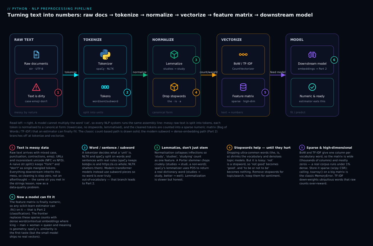
The six badges mark the decisions that actually bite a beginner: raw text is dirty and cleaning is step zero (1); a “token” can be a word, a sentence or a subword and the choice matters (2); lemmatization returns real words where stemming returns stumps (3); stopword removal is lossy and sometimes catastrophic (4); the resulting matrix is wide and almost all zeros (5); and the frontier swaps these sparse counts for dense embeddings (6). We will walk each one.
Text is messy data
Before you tokenize anything, look honestly at what raw text actually contains. The single most common beginner mistake is to assume text is clean and reach straight for str.split(). Here is what real text throws at you, and why the naive approach breaks on every row.
| Mess | Example | Why it breaks naive code |
|---|---|---|
| Mixed case | "Apple", "apple", "APPLE" |
Three different features unless you lowercase — but lowercasing kills Apple (company) vs apple (fruit) |
| Punctuation glued to words | "York!", "good.", "(hi)" |
split() keeps the ! and . attached, so "good" and "good." are different tokens |
| Contractions | "don't", "I'm", "we'll" |
Is "don't" one token or do + n't? Naive split says one; the meaning is two (do + not) |
| Multi-word units | "New York", "machine learning" |
split() shatters them into New+York; the meaning lives in the pair |
| URLs, emails, handles | "bob@x.io", "https://a.co/b", "@user" |
Contain ., /, @ — punctuation-based splitting rips them apart |
| Emoji & symbols | "great 👍", "5 °C" |
One “character” can be several code points (len("👨👩👧👦") == 7) |
| Unicode variants | "café" as NFC vs NFD |
Two byte-spellings compare unequal; "é" != "é" |
| Encoding damage | "café", "it’s" |
UTF-8 bytes decoded as latin-1 — mojibake, no exception raised |
| Whitespace & newlines | " a\t b\n" |
Tabs, non-breaking spaces (\xa0), trailing newlines from file reads |
Watch a naive split fall apart on a single realistic sentence:
text = "Don't email me at bob@x.io — I'm in New York! Visit https://a.co/b."
print(text.split())
["Don't", 'email', 'me', 'at', 'bob@x.io', '—', "I'm", 'in', 'New', 'York!', 'Visit', 'https://a.co/b.']
Count the damage. "York!" carries a stuck exclamation mark, so it will never match the token "York". "https://a.co/b." has a trailing period that corrupts the URL. "Don't" and "I'm" are single tokens, hiding the negation n't and the verb 'm. And "New" and "York" are two separate tokens — the place name is gone. Every one of these is a feature your model will now get wrong. str.split() is a fine tool for a clean CSV field; it is the wrong tool for language.
This is exactly the strings-lesson material coming back as a data problem. Before tokenizing, real pipelines normalize the raw string: unicodedata.normalize("NFC", text) to unify accent spellings, .strip() to kill trailing whitespace, an explicit encoding="utf-8" at every file boundary so you never decode UTF-8 as latin-1. Clean the str, then tokenize.
Tokenization: what is a token?
Tokenization is the act of deciding what a “unit” of text is. It sounds trivial and is not. Every choice you make here propagates through the entire pipeline, because tokens are the atoms everything downstream counts.
There are three granularities, and real systems use all three:
| Granularity | A token is… | Example: "I don't like New York." |
Used by |
|---|---|---|---|
| Word | a word or symbol | I · do · n't · like · New · York · . |
Classic NLP, BoW, TF-IDF |
| Sentence | a whole sentence | ["I don't like New York."] |
Summarization, translation, sentence embeddings |
| Subword | a frequent character chunk | I · do · n · 't · like · New · York · . (and unhappiness → un + happi + ness) |
All modern transformers (Part 2) |
Word tokenization is what this lesson uses. Subword tokenization is the modern path and deserves a flag now: transformer models (BERT, GPT, and friends) never tokenize on words, because a fixed word vocabulary can never cover every name, typo, or new coinage — a word it has never seen becomes <UNK> and its meaning is lost. Subword tokenizers (BPE, WordPiece, SentencePiece) instead learn a vocabulary of frequent character chunks, so "tokenization" might become token + ization and a word the model has never seen is still spelled out of pieces it knows. No word is ever truly out-of-vocabulary. We build word-based features here because they are interpretable and they are what BoW/TF-IDF need; Part 2 explains why the frontier moved to subwords.
NLTK vs spaCy tokenizers on the same text
Both libraries do far better than split(), but they disagree in instructive ways. NLTK’s word_tokenize is rule-based (a Treebank tokenizer); spaCy’s tokenizer is also rule-based but tuned for the messy real web.
from nltk.tokenize import word_tokenize, sent_tokenize
import spacy

s = "Don't email me at bob@x.io — I'm in New York! Visit https://a.co/b."

print("NLTK:", word_tokenize("Don't email me at bob@x.io in New York!"))

nlp = spacy.load("en_core_web_sm")
print("spaCy:", [t.text for t in nlp(s)])
NLTK:  ['Do', "n't", 'email', 'me', 'at', 'bob', '@', 'x.io', 'in', 'New', 'York', '!']
spaCy: ['Do', "n't", 'email', 'me', 'at', 'bob@x.io', '—', 'I', "'m", 'in', 'New', 'York', '!', 'Visit', 'https://a.co/b', '.']
Both correctly split the contraction Don't into Do + n't — that is the whole reason you don’t hand-roll this. But look at the email: NLTK shatters bob@x.io into three tokens (bob, @, x.io), while spaCy keeps it whole. spaCy also keeps the URL https://a.co/b as a single token. For anything touching web text — reviews, tweets, support tickets — spaCy’s tokenizer is materially better out of the box. (Neither, by default, joins New York into one token; multi-word entities are recovered later by the named-entity recognizer, not the tokenizer.)
They disagree in both directions, though, and the disagreements are worth knowing before you pick one. Run the same tricky strings through all three:
| Input | str.split() |
NLTK word_tokenize |
spaCy |
|---|---|---|---|
don't |
["don't"] ❌ |
['do', "n't"] ✅ |
['do', "n't"] ✅ |
U.K. |
['U.K.'] |
['U.K', '.'] ❌ (drops the dot) |
['U.K.'] ✅ |
$3.50 |
['$3.50'] |
['$', '3.50'] ✅ |
['$', '3.50'] ✅ |
bob@x.io |
['bob@x.io'] |
['bob', '@', 'x.io'] ❌ |
['bob@x.io'] ✅ |
https://a.co/b |
['https://a.co/b'] |
['https', ':', '//a.co/b'] ❌ |
['https://a.co/b'] ✅ |
state-of-the-art |
['state-of-the-art'] |
['state-of-the-art'] |
['state', '-', 'of', '-', 'the', '-', 'art'] |
New York |
['New', 'York'] |
['New', 'York'] |
['New', 'York'] |
The pattern: spaCy protects web artifacts (emails, URLs, abbreviations) but splits hyphenated compounds, while NLTK does the reverse — it keeps state-of-the-art whole but tears apart every URL and email. There is no universally “correct” tokenization; there is only the one that matches your data. For social/web text, spaCy’s choices cost you less.
Sentence tokenization is its own hard problem, because a period is not a reliable sentence boundary — "Dr.", "U.K.", "3.50" all contain one. NLTK’s sent_tokenize handles the common abbreviations:
print(sent_tokenize("Dr. Smith went to Washington. He didn't stay long! Cost: $3.50."))
['Dr. Smith went to Washington.', "He didn't stay long!", 'Cost: $3.50.']
Three sentences, and it correctly did not break after "Dr." or inside "$3.50". spaCy exposes the same via doc.sents (an iterator of Span objects), computed by its dependency parser rather than by rules.
spaCy tokens carry attributes
The reason spaCy is a “pipeline” and not just a tokenizer is that every token is a rich object, not a bare string. Each Token already knows what kind of thing it is, which is what lets you filter cleanly in the normalize step:
for t in nlp("I'm emailing bob@x.io about 3 cats."):
    print(f"{t.text!r:12} stop={t.is_stop!s:5} punct={t.is_punct!s:5} "
          f"url={t.like_url!s:5} email={t.like_email!s:5} alpha={t.is_alpha}")
'I'          stop=True  punct=False url=False email=False alpha=True
"'m"         stop=True  punct=False url=False email=False alpha=False
'emailing'   stop=False punct=False url=False email=False alpha=True
'bob@x.io'   stop=False punct=False url=False email=True  alpha=False
'about'      stop=True  punct=False url=False email=False alpha=True
'3'          stop=False punct=False url=False email=False alpha=False
'cats'       stop=False punct=False url=False email=False alpha=True
'.'          stop=False punct=True  url=False email=False alpha=False
is_stop, is_punct, like_url, like_email, is_alpha — these boolean flags are precomputed, so “keep only real alphabetic content words” is a one-line comprehension. NLTK gives you none of this for free; you assemble it from separate function calls and your own regex. This is the core ergonomic difference between the two libraries, and we will lean on it in the lab.
Normalization: collapsing variety
After tokenizing you have units, but the same meaning still wears many surface forms: Run, run, runs, running, ran. To a raw counter those are five different features, splitting the signal five ways. Normalization collapses surface forms into a canonical form so that meaning, not spelling, drives the counts. There are four moves, and each has an honest downside.
Lowercasing (and when case is signal)
Lowercasing is the cheapest normalization: "Apple".lower() == "apple". It halves your vocabulary at a stroke and is right almost always — except when case carries meaning. Apple (the company) and apple (the fruit); US (the country) and us (the pronoun); March (month) and march (verb). Named-entity recognition (NER) depends on case — a capitalized word mid-sentence is a strong signal of a proper noun. So the rule is: lowercase for topic modelling, search, and bag-of-words classification; preserve case if you are doing NER or anything where proper nouns matter. And crucially, order matters — lowercase after the linguistic steps that need case, not before, a trap we will hit live in the lab.
Stopword removal (and when it destroys meaning)
Stopwords are ultra-common words — the, is, a, of, and — that appear in nearly every document and so carry little topic signal. Removing them shrinks the vocabulary and denoises topic models and search indexes. NLTK ships a list:
from nltk.corpus import stopwords
sw = set(stopwords.words("english"))
print(len(sw), "stopwords; sample:", sorted(sw)[:10])
198 stopwords; sample: ['a', 'about', 'above', 'after', 'again', 'against', 'ain', 'all', 'am', 'an']
Now the honest part every tutorial skips. Stopword removal is lossy, and sometimes catastrophic. The word not is on that list of 198. Watch what removing stopwords does to a sentence whose whole meaning is negation:
sentence = "This is not a very good movie and I would not recommend it"
kept = [w for w in sentence.lower().split() if w not in sw]
print(kept)
['good', 'movie', 'would', 'recommend']
A scathing review just became good movie would recommend — the sentiment is inverted. And the classic demonstration:
print([w for w in "to be or not to be".split() if w not in sw])
[]
Hamlet’s line reduces to nothing — every word is a stopword. The lesson is not “never remove stopwords”; it is know your task. Remove them for topic modelling, keyword search and document clustering, where common glue words are noise. Keep them for sentiment analysis, authorship attribution, and anything where not, no, never, and function words carry the signal. When in doubt, measure both.
| Task | Remove stopwords? | Why |
|---|---|---|
| Topic modelling / clustering | Yes | Common words dominate counts and blur topics |
| Keyword search / TF-IDF ranking | Usually | TF-IDF already down-weights them; removal is a cheap extra |
| Sentiment analysis | No | not, no, never invert meaning and are stopwords |
| Authorship attribution | No | Function-word frequency is the author’s fingerprint |
| Machine translation / transformers | No | Modern models need every token; they learn what to ignore |
Stemming vs lemmatization
This is the heart of normalization, and the place the two approaches genuinely differ. Both reduce inflected words to a base form; they do it with opposite philosophies.
Stemming chops affixes with crude rules and no dictionary. The Porter stemmer (1980) is a cascade of suffix-stripping rules: strip -ing, strip -es, collapse -y to -i. It is fast, language-light, and it frequently produces non-words, because it does not know what a word is — it only knows suffixes.
Lemmatization maps a word to its dictionary headword (its lemma) using a real vocabulary and, ideally, the word’s part of speech. better → good (with adjective POS); mice → mouse; was → be. It is slower and needs linguistic resources, but every output is a real word.
Watch them side by side on the same words. This single table is the argument:
from nltk.stem import PorterStemmer, SnowballStemmer, WordNetLemmatizer
import spacy
porter, snow, wnl = PorterStemmer(), SnowballStemmer("english"), WordNetLemmatizer()
nlp = spacy.load("en_core_web_sm")
| Word | Porter stem | Snowball stem | WordNet lemma (verb) | WordNet lemma (noun) | spaCy lemma (in context) |
|---|---|---|---|---|---|
studies |
studi ❌ |
studi ❌ |
study |
study |
study |
studying |
studi ❌ |
studi ❌ |
study |
studying |
study |
cats |
cat |
cat |
cat |
cat |
cat |
better |
better |
better |
better |
better |
well ✅ |
running |
run |
run |
run |
running |
run |
ran |
ran ❌ |
ran ❌ |
run |
ran |
run |
was |
wa ❌ |
was |
be |
wa ❌ |
be |
mice |
mice ❌ |
mice ❌ |
mice |
mouse |
mouse ✅ |
feet |
feet ❌ |
feet ❌ |
feet |
foot |
foot ✅ |
organization |
organ ❌ |
organ ❌ |
organization |
organization |
organization |
happily |
happili ❌ |
happili ❌ |
happily |
happily |
happily |
generous |
gener ❌ |
generous |
generous |
generous |
generous |
Read the failures. Porter turns studies into studi, happily into happili, generous into gener, and — the scary one — organization into organ, silently merging a word about companies with a word about body parts. It cannot fix irregulars: ran, mice, feet, was come out unchanged or mangled (wa), because there is no -ing/-s suffix to chop. spaCy’s context-aware lemmatizer gets all of them right, including the ones that require knowing the part of speech: better → well, mice → mouse, feet → foot.
The reason WordNet has two columns is the sharp edge: WordNetLemmatizer defaults to treating every word as a noun. wnl.lemmatize("running") returns running (the noun) unless you pass pos='v', in which case you get run. You must tell it the part of speech, which means you must run a POS tagger first — exactly the wiring spaCy does for you. Here is spaCy lemmatizing in real sentence context, choosing the POS itself:
for t in nlp("The studies were running better after the mice organized their feet."):
    print(f"{t.text:10} -> {t.lemma_:9} ({t.pos_})")
The        -> the       (DET)
studies    -> study     (NOUN)
were       -> be        (AUX)
running    -> run       (VERB)
better     -> well      (ADV)
mice       -> mouse     (NOUN)
organized  -> organize  (VERB)
feet       -> foot      (NOUN)
Every output is a real dictionary word, and the POS was inferred from context. That is why, for a production pipeline, spaCy lemmatization is the default and stemming is the fast, dirty fallback you reach for only when speed matters more than correctness (e.g., a huge search index where studi matching studies and studying is a feature, not a bug).
| Stemming | Lemmatization | |
|---|---|---|
| Method | Rule-based suffix chopping | Dictionary lookup + POS |
| Output | Often a non-word (studi, gener) |
Always a real word (study, good) |
| Needs POS? | No | Yes (for correctness) |
| Handles irregulars? | No (ran→ran, mice→mice) |
Yes (ran→run, mice→mouse) |
| Speed | Very fast | Slower (needs the model) |
| Best tool | NLTK PorterStemmer / SnowballStemmer |
spaCy token.lemma_ |
| When | Search indexes, huge corpora, speed-critical | Almost everything else |
Punctuation and numbers
The last normalization decisions are what to do with punctuation and digits. Usually you drop pure punctuation (it rarely carries topic signal for BoW) and either drop numbers or replace them with a placeholder token like <NUM> (so "iPhone 12" and "iPhone 13" share a feature). With spaCy this is trivial because the flags are precomputed — not tok.is_punct and not tok.is_space and tok.is_alpha keeps only alphabetic content, dropping punctuation, whitespace and numbers in one filter. Just remember is_alpha is False for "3", "3.50", and "bob@x.io", so an is_alpha filter silently removes those too — a decision you want to make on purpose.
NLTK vs spaCy: the teaching toolkit vs the production pipeline
You have now met both libraries piecemeal. Here is the head-to-head, because choosing the right one is a real decision.
| NLTK (2001) | spaCy (2015) | |
|---|---|---|
| Philosophy | Modular toolkit — one function per concept | Opinionated pipeline — one nlp object does everything |
| Design goal | Teaching, research, flexibility | Production speed and ergonomics |
| Tokenizer | word_tokenize, sent_tokenize (good) |
Built into nlp() (better on web text) |
| Stemming | ✅ Porter, Snowball, Lancaster | ❌ None (deliberate — lemmas instead) |
| Lemmatization | WordNetLemmatizer (needs manual POS) |
✅ token.lemma_ (automatic POS) |
| POS tagging | nltk.pos_tag (separate call) |
✅ token.pos_ / token.tag_ (built in) |
| Dependency parse | ❌ (limited) | ✅ token.dep_, token.head |
| Named entities | Basic chunker | ✅ doc.ents (strong) |
| Word vectors | ❌ (bring your own) | ✅ in md/lg models |
| Output | Python lists and strings | Rich Doc / Token / Span objects |
| Speed on big data | Slower, Python-level | Fast (Cython), nlp.pipe batching |
| Best for | Learning the concepts, quick experiments, WordNet | Shipping a real pipeline |
The one-line summary: learn with NLTK, ship with spaCy. NLTK makes every step explicit, which is perfect for understanding; spaCy fuses the steps into a fast, well-engineered object, which is what you want in a service. They are not rivals so much as different points on the “explicit vs done-for-you” axis, and mature codebases often use both — spaCy for the pipeline, NLTK for its unmatched WordNet access.
The spaCy object model
When you call nlp(text), spaCy runs a pipeline of components in order and returns a Doc. You can see the components:
nlp = spacy.load("en_core_web_sm")
print(nlp.pipe_names)
['tok2vec', 'tagger', 'parser', 'attribute_ruler', 'lemmatizer', 'ner']
Each component annotates the tokens: tagger sets POS, parser sets dependencies and sentence boundaries, lemmatizer sets lemmas, ner finds entities. The result is three object types you will use constantly:
| Object | Is | Get it from | Key attributes |
|---|---|---|---|
Doc |
The whole processed text | nlp(text) |
Iterable of tokens; .sents, .ents, .noun_chunks |
Token |
One token | doc[i] |
.text, .lemma_, .pos_, .tag_, .dep_, .head, .is_stop, .is_alpha, .like_url |
Span |
A slice of tokens | doc[i:j], an entity, a sentence |
.text, .label_ (for entities), .root |
Here is the full linguistic pipeline on one sentence — POS tags, the dependency parse (each token’s grammatical head), and named entities — all from a single nlp() call:
doc = nlp("Apple is looking at buying a U.K. startup for $1 billion in 2027.")
for t in doc:
    print(f"{t.text:8} {t.pos_:6} {t.dep_:10} head={t.head.text}")
print("ENTITIES:", [(e.text, e.label_) for e in doc.ents])
Apple    PROPN  nsubj      head=looking
is       AUX    aux        head=looking
looking  VERB   ROOT       head=looking
at       ADP    prep       head=looking
buying   VERB   pcomp      head=at
a        DET    det        head=U.K.
U.K.     PROPN  dobj       head=buying
startup  NOUN   advcl      head=looking
for      ADP    prep       head=startup
$        SYM    quantmod   head=billion
1        NUM    compound   head=billion
billion  NUM    pobj       head=for
in       ADP    prep       head=startup
2027     NUM    pobj       head=in
.        PUNCT  punct      head=looking
ENTITIES: [('Apple', 'ORG'), ('U.K.', 'GPE'), ('$1 billion', 'MONEY'), ('2027', 'DATE')]
In one pass spaCy recovered that Apple is a proper noun and the subject of looking, that $1 billion is a MONEY entity spanning three tokens, that 2027 is a DATE, and that U.K. is a geopolitical entity (GPE) — and it kept U.K. and $1 billion as coherent units the word tokenizer alone would have split. spacy.explain("GPE") returns “Countries, cities, states” if you forget a label. This is why spaCy is a “pipeline”: one call, many annotations.
Named-entity types and POS tags
Two reference tables you will return to. The Universal POS tags (coarse, token.pos_):
| Tag | Meaning | Example | Tag | Meaning | Example | |
|---|---|---|---|---|---|---|
NOUN |
common noun | cat |
ADP |
adposition | in, to |
|
PROPN |
proper noun | Apple |
DET |
determiner | the, a |
|
VERB |
verb | run |
PRON |
pronoun | she |
|
AUX |
auxiliary | is, was |
NUM |
numeral | 2027 |
|
ADJ |
adjective | good |
PUNCT |
punctuation | . |
|
ADV |
adverb | quickly |
SYM |
symbol | $ |
Common spaCy entity labels (ent.label_):
| Label | Means | Label | Means |
|---|---|---|---|
PERSON |
People | GPE |
Countries, cities, states |
ORG |
Companies, agencies | LOC |
Non-GPE locations, mountains |
MONEY |
Monetary values | DATE |
Absolute or relative dates |
PRODUCT |
Objects, vehicles | TIME |
Times smaller than a day |
CARDINAL |
Numerals | PERCENT |
Percentages |
Batch processing with nlp.pipe
The one performance rule for spaCy: never loop nlp(text) over a big list. Each call has fixed overhead; nlp.pipe streams documents through the pipeline in efficient batches (and can multiprocess with n_process):
texts = ["First document.", "Second one is longer.", "Third."]
for d in nlp.pipe(texts):
    print(f"{d.text!r:30} -> {len(d)} tokens")
'First document.'              -> 3 tokens
'Second one is longer.'        -> 4 tokens
'Third.'                       -> 2 tokens
And when you only need some annotations, disable the components you don’t use — the parser and NER are the expensive ones:
fast = spacy.load("en_core_web_sm", disable=["parser", "ner"])
print(fast.pipe_names)   # ['tok2vec', 'tagger', 'attribute_ruler', 'lemmatizer']
For a lemmatize-and-vectorize job you don’t need the parser or NER at all, so disabling them is free speed. We do exactly that in the lab.
Regex still earns its place
Not every cleaning step deserves a full NLP pipeline. For the crude, structural stuff — stripping HTML tags, masking URLs and emails, collapsing repeated whitespace — a regex from the datetime & regex lesson is faster and simpler than any tokenizer. Regex runs before tokenization, as a raw-string cleanup:
import re
text = "Check   https://a.co NOW!!! Email  bob@x.io  😊"
text = re.sub(r"https?://\S+", " <URL> ", text)   # mask URLs
text = re.sub(r"\S+@\S+", " <EMAIL> ", text)       # mask emails
text = re.sub(r"\s+", " ", text).strip()            # collapse whitespace
print(text)   # => Check <URL> NOW!!! Email <EMAIL> 😊
The division of labour: regex for structural noise, tokenizer for linguistic units. Replacing every URL with a single <URL> token before tokenizing means a thousand different links collapse into one feature — often exactly what you want. Just resist the temptation to tokenize entirely with regex; re.findall(r"\w+", text) is a naive tokenizer that re-introduces every contraction and abbreviation bug spaCy already solved.
Representing text as numbers: Bag of Words and TF-IDF
Now the payoff. You have clean, normalized tokens; the model wants numbers. The bridge is vectorization — turning each document into a fixed-length vector of counts or weights, one dimension per vocabulary word.
Bag of Words
The simplest representation is Bag of Words (BoW): build a vocabulary of every word in the corpus, then represent each document as the vector of how many times each vocabulary word appears. “Bag” because word order is discarded — "dog bites man" and "man bites dog" produce identical vectors. scikit-learn’s CountVectorizer does the whole thing:
from sklearn.feature_extraction.text import CountVectorizer
corpus = ["the cat sat on the mat",
          "the dog sat on the log",
          "the cat and the dog played"]
cv = CountVectorizer()
X = cv.fit_transform(corpus)
print(cv.get_feature_names_out().tolist())
print(X.toarray())
['and', 'cat', 'dog', 'log', 'mat', 'on', 'played', 'sat', 'the']
[[0 1 0 0 1 1 0 1 2]
 [0 0 1 1 0 1 0 1 2]
 [1 1 1 0 0 0 1 0 2]]
Nine vocabulary words become nine columns; each row is a document. Row 0 ("the cat sat on the mat") has the twice (last column = 2), cat/mat/on/sat once, and zeros elsewhere. That 3×9 grid of integers is something a model can finally multiply. Notice two of CountVectorizer’s silent defaults already at work: it lowercased everything, and its default token pattern dropped one-character tokens and punctuation (there is no a-as-a-letter column). Those defaults surprise people, so keep them in mind:
| Default | Value | Consequence | When it bites |
|---|---|---|---|
lowercase |
True |
Apple/apple/APPLE merge into one feature |
You wanted case as signal (NER, tickers like US) |
token_pattern |
(?u)\b\w\w+\b |
Tokens under 2 chars and all punctuation are dropped | You needed "a", "I", "3", emoji, or "C++" |
stop_words |
None |
Stopwords are kept by default | You assumed they were removed |
ngram_range |
(1, 1) |
Unigrams only — no word order | "not good" collapses to two lone words |
binary |
False |
Counts, not presence | You wanted 0/1 occurrence flags |
max_features |
None |
Full vocabulary — can be huge | Memory blows up on a big corpus |
Watch the token-pattern default silently eat data: CountVectorizer().fit(["I am a data scientist! 3 cats"]) yields the vocabulary ['am', 'cats', 'data', 'scientist'] — the I, a, and 3 are gone because they are shorter than two word-characters. If you need single characters or digits, pass token_pattern=r"(?u)\b\w+\b". These defaults matter — more below.
Why TF-IDF beats raw counts
BoW has a bias: it rewards frequency blindly. The word the appears in every document and dominates every count vector, yet it tells you nothing about what a document is about. Rare words like mat and played are far more informative, but raw counts drown them out. TF-IDF fixes this by down-weighting words that appear everywhere.
TF-IDF = Term Frequency × Inverse Document Frequency. The intuition:
- TF (term frequency): how often the word appears in this document. More = more relevant to this doc.
- IDF (inverse document frequency): how rare the word is across all documents. A word in every document has low IDF (uninformative); a word in one document has high IDF (distinctive).
Multiply them and you get a weight that is high only for words that are frequent here but rare elsewhere — the words that actually characterize a document. Both vectorizers are ordinary scikit-learn transformers with the same fit/transform contract as the scalers and encoders from the scikit-learn preprocessing lesson, so a TfidfVectorizer drops straight into a Pipeline in front of a classifier — fit on train, transform test, no leakage. scikit-learn’s smoothed formula is:
idf(t) = ln[ (1 + N) / (1 + df(t)) ] + 1        (N = number of documents, df = docs containing t)
tfidf(t, d) = tf(t, d) × idf(t)                  (then each document vector is L2-normalized)
You can watch the IDF do its job. On the same three-document corpus:
from sklearn.feature_extraction.text import TfidfVectorizer
tv = TfidfVectorizer()
Xt = tv.fit_transform(corpus)
for term, idf in sorted(zip(tv.get_feature_names_out(), tv.idf_), key=lambda p: p[1]):
    print(f"{term:8} idf={idf:.3f}")
the      idf=1.000
cat      idf=1.288
dog      idf=1.288
on       idf=1.288
sat      idf=1.288
and      idf=1.693
log      idf=1.693
mat      idf=1.693
played   idf=1.693
the (in all 3 docs) gets the lowest IDF, 1.000 — check the math: ln(4/4) + 1 = ln(1) + 1 = 1.000. Words in one document (mat, played) get the highest, ln(4/2) + 1 = 1.693. IDF is the knob that shrinks ubiquitous words and amplifies distinctive ones.
Here is an honest nuance most tutorials gloss over. Even after TF-IDF, on this tiny corpus the still has a high weight in row 0, because it appears twice (TF = 2) and there are only three documents, so its low IDF can’t fully suppress its high frequency. IDF narrows the gap; it does not erase it. On a realistic corpus of thousands of documents where the appears in nearly all of them, its IDF collapses toward the floor and TF-IDF crushes it — and in practice you also remove stopwords explicitly. TF-IDF and stopword removal are complementary, not redundant. (Watch the vanish entirely in the lab, where we strip stopwords first.)
Ranking the top-weighted terms per document shows TF-IDF surfacing the distinctive words:
vocab = tv.get_feature_names_out()
for i, row in enumerate(Xt.toarray()):
    top = sorted(zip(vocab, row), key=lambda p: -p[1])[:3]
    print(f"doc {i}:", [(t, round(float(w), 3)) for t, w in top if w > 0])
doc 0: [('the', 0.581), ('mat', 0.492), ('cat', 0.374)]
doc 1: [('the', 0.581), ('log', 0.492), ('dog', 0.374)]
doc 2: [('the', 0.554), ('and', 0.469), ('played', 0.469)]
mat characterizes doc 0, log characterizes doc 1, played characterizes doc 2 — exactly the distinctive words, now that the is (partly) discounted and the truly unique words rise. CountVectorizer and TfidfVectorizer share almost all parameters; the difference is only the weighting:
| Parameter | Does | Common value |
|---|---|---|
lowercase |
Lowercase before tokenizing | True (default) |
stop_words |
Drop a stopword list | "english" or a custom set |
ngram_range |
Which n-grams to include | (1, 1) unigrams; (1, 2) uni+bigrams |
max_features |
Cap vocabulary to the top-K by frequency | 10000 |
min_df |
Ignore terms in fewer than this many docs | 2 (drop hapax typos) |
max_df |
Ignore terms in more than this fraction of docs | 0.9 (drop corpus-specific stopwords) |
token_pattern |
Regex defining a token | default (?u)\b\w\w+\b (2+ word chars) |
sublinear_tf (TF-IDF) |
Use 1 + log(tf) instead of raw tf |
True for long docs |
min_df and max_df are the quiet workhorses: min_df=2 drops every word that appears in only one document (mostly typos and noise), and max_df=0.9 drops words appearing in over 90% of documents (corpus-specific stopwords you never listed). Together they clean the vocabulary without a hand-maintained list.
n-grams: recovering a little word order
BoW throws away order, which loses "not good" — the two words survive but their pairing does not, and to a unigram model "not good" and "good" look almost the same. n-grams claw back local order by treating adjacent word runs as tokens. A bigram is a 2-word sequence:
reviews = ["the movie was not good", "the movie was good"]
print("unigrams:", CountVectorizer().fit(reviews).get_feature_names_out().tolist())
print("uni+bi:  ", CountVectorizer(ngram_range=(1, 2)).fit(reviews).get_feature_names_out().tolist())
unigrams: ['good', 'movie', 'not', 'the', 'was']
uni+bi:   ['good', 'movie', 'movie was', 'not', 'not good', 'the', 'the movie', 'was', 'was good', 'was not']
With ngram_range=(1, 2) the vocabulary now contains not good and was good as distinct features — a sentiment model can finally tell the two reviews apart. The cost is vocabulary explosion: bigrams multiply the feature count several-fold, and trigrams more again. n-grams are the cheapest way to add a little context to BoW, and max_features or min_df is how you stop them blowing up.
The sparse, high-dimensional reality
One structural fact defines classical text vectors: the matrix is wide and almost entirely zeros. Your vocabulary might be 50,000 words, but any single tweet uses maybe 20 of them — so 49,980 of its 50,000 columns are zero. Storing that as a dense array wastes almost all the memory on zeros. scikit-learn returns a sparse matrix (SciPy CSR) that stores only the non-zeros. The scale is not subtle:
import numpy as np
from sklearn.feature_extraction.text import TfidfVectorizer
rng = np.random.default_rng(0)
pool = [f"term{i}" for i in range(5000)]
docs = [" ".join(rng.choice(pool, size=rng.integers(20, 60))) for _ in range(2000)]
X = TfidfVectorizer().fit_transform(docs)
cells = X.shape[0] * X.shape[1]
print(f"shape={X.shape}, non-zeros={X.nnz:,}, density={X.nnz/cells:.2%}")
sparse_mb = (X.data.nbytes + X.indices.nbytes + X.indptr.nbytes) / 1e6
print(f"sparse: {sparse_mb:.1f} MB   dense would be: {cells*8/1e6:.0f} MB")
shape=(2000, 5000), non-zeros=79,085, density=0.79%
sparse: 1.0 MB   dense would be: 80 MB
Under 1% of the cells are non-zero, and the sparse representation is 1 MB where the dense version would be 80 MB — an 80× saving, and that is a small example. This is why X.toarray() is a trap: on a real corpus (100k docs × 50k vocab) the dense array is 40 GB and the call is an instant MemoryError. Keep the matrix sparse; scikit-learn’s estimators accept sparse input directly. The high dimensionality also motivates everything in Part 2 — the “curse of dimensionality” is why dense embeddings, which pack meaning into a few hundred dimensions instead of tens of thousands, took over.
Using the vectors: cosine similarity
Once documents are vectors, “how similar are these two documents?” becomes geometry — and the standard measure is cosine similarity, the cosine of the angle between two vectors. It ranges from 0 (no shared terms, orthogonal) to 1 (identical direction), and it ignores document length because it compares direction, not magnitude — a paragraph and a one-liner about the same topic still score high. This is the engine under document search, deduplication, and “related articles”:
from sklearn.metrics.pairwise import cosine_similarity
sim = cosine_similarity(Xt)          # Xt = the TF-IDF matrix from above
print(sim.round(3))
[[1.    0.618 0.455]
 [0.618 1.    0.455]
 [0.455 0.455 1.   ]]
The diagonal is 1 (every document is identical to itself), and doc 0 and doc 1 ("the cat sat on the mat" / "the dog sat on the log") score highest off-diagonal at 0.618 because they share sat, on and the — TF-IDF on top of cosine is a complete, if classical, search engine in three lines. But notice the ceiling this hits: docs 0 and 1 are “similar” only because they reuse words. Swap cat for feline and the similarity would crater to near zero, even though the meaning is nearly identical — cosine on sparse count vectors sees shared tokens, never shared meaning. That blind spot is the exact motivation for the next section.
A first look at word embeddings
BoW and TF-IDF have a blind spot that no amount of tuning fixes: every word is an island. In a TF-IDF matrix, cat and dog are as unrelated as cat and democracy — each is its own orthogonal column, and the representation knows nothing about meaning. king and queen share zero similarity unless they literally co-occur. This is the wall that ended the classical era.
Word embeddings knock it down. The idea (word2vec, 2013; GloVe, 2014) is to represent each word as a dense vector of a few hundred real numbers — say 300 — learned so that words used in similar contexts get similar vectors. “You shall know a word by the company it keeps”: because cat and dog appear in similar sentences (both get fed, both are pets), they land near each other in the vector space. Meaning becomes geometry.
| Sparse (BoW / TF-IDF) | Dense (embeddings) | |
|---|---|---|
| Dimensions | 10k–100k (vocabulary size) | 50–300 (fixed) |
| Values | Mostly zero, counts/weights | All non-zero, learned reals |
cat vs dog |
Orthogonal — unrelated | Close — similar vectors |
| Captures meaning? | No, only co-occurrence | Yes, similarity is geometric |
| Interpretable? | Yes (each column is a word) | No (dimensions are latent) |
| Made by | Counting | Training a shallow net (word2vec) |
The famous demonstration is that these vectors support analogies as arithmetic: king − man + woman ≈ queen, and Paris − France + Italy ≈ Rome. The relationship “capital of” and the relationship “male→female” become consistent directions in the space. No one programmed that; it falls out of training on enough text.
spaCy exposes vector similarity via .similarity, which is your first hands-on taste — but with a critical honest caveat. The small model en_core_web_sm ships no real word vectors to stay tiny (~12 MB). Ask it for similarity and it warns you:
import spacy
nlp = spacy.load("en_core_web_sm")
print("has real vectors?", nlp.vocab.vectors_length > 0)   # => False
print(nlp("cat")[0].similarity(nlp("dog")[0]))
has real vectors? False
UserWarning: [W007] The model you're using has no word vectors loaded, so the result
of the Token.similarity method will be based on the tagger, parser and NER, which may
not give useful similarity judgements. ...
0.742
It returns a number (0.742) computed from context tensors, but the W007 warning is telling you the truth: this is not a real word-embedding similarity. For genuine .similarity, load en_core_web_md or en_core_web_lg (which bundle 300-d GloVe vectors), or use the gensim library’s word2vec. We deliberately do not download those here — but now you know exactly what the warning means and why the small model raises it.
Which model you load is a real trade-off between size, speed and whether you get vectors at all:
| Model | Size | Word vectors | .similarity |
Use when |
|---|---|---|---|---|
en_core_web_sm |
~12 MB | ❌ none (context tensors) | Warns (W007), unreliable | Tokenize, POS, lemma, NER — no similarity needed |
en_core_web_md |
~40 MB | ✅ 300-d GloVe (20k unique) | Works | Similarity on a budget; most projects |
en_core_web_lg |
~560 MB | ✅ 300-d GloVe (500k+ unique) | Best static | Similarity quality matters, RAM available |
en_core_web_trf |
~430 MB | Contextual (transformer) | Via transformer | Highest accuracy; the bridge to Part 2 |
The small model is the right default for this lesson — every pipeline stage except .similarity works perfectly on it, at a twelfth of the download. Reach for md the moment you actually need semantic similarity, and note that trf (a RoBERTa transformer under a spaCy wrapper) is exactly the contextual-embedding technology Part 2 is about.
These static embeddings — one fixed vector per word — still have a limit: bank gets the same vector in “river bank” and “savings bank.” The fix is contextual embeddings, where a transformer produces a different vector for a word depending on its sentence. That is the bridge to Part 2: subword tokenization feeds a transformer that outputs context-aware vectors, and the whole sparse-count pipeline you just learned becomes the baseline those models are measured against. Understand this pipeline and the leap to transformers is a step, not a cliff.
Hands-on lab
You will build the real pipeline end to end: five raw, messy documents → spaCy clean + lemmatize + drop stopwords → TfidfVectorizer → the vocabulary and the top-weighted terms per document — then contrast stemming against lemmatization and BoW against TF-IDF on the same text. Everything runs locally and every output below is real.
⚠️ This lab installs packages and downloads a ~12 MB language model. Do it in a virtual environment so it never touches your system Python.
Step 1 — Create an isolated environment. spaCy, NLTK and scikit-learn are substantial; a venv keeps them contained.
mkdir -p ~/pylab/nlp && cd ~/pylab/nlp
python3.12 -m venv .venv
source .venv/bin/activate           # Windows: .venv\Scripts\activate
python -m pip install --upgrade pip
pip install nltk spacy scikit-learn
Step 2 — Download the models and corpora. spaCy’s model and NLTK’s data are separate downloads, not part of the pip install.
python -m spacy download en_core_web_sm
python -c "import nltk; [nltk.download(p) for p in ['stopwords','wordnet','punkt','punkt_tab','averaged_perceptron_tagger_eng']]"
Each NLTK resource powers a specific feature, and you only download what you use:
| Resource | Powers | Missing it raises |
|---|---|---|
punkt / punkt_tab |
word_tokenize, sent_tokenize |
LookupError: Resource punkt not found |
stopwords |
stopwords.words("english") |
LookupError: Resource stopwords not found |
wordnet |
WordNetLemmatizer |
LookupError: Resource wordnet not found |
averaged_perceptron_tagger_eng |
nltk.pos_tag |
LookupError: ...averaged_perceptron_tagger... |
If the NLTK download fails with an SSL
CERTIFICATE_VERIFY_FAILEDerror (common on macOS), point it at certifi’s bundle first:export SSL_CERT_FILE=$(python -c "import certifi; print(certifi.where())")and re-run. If a corporate proxy blocks it entirely, the pipeline still runs — you just lose the NLTK stemmer comparison in Step 4; spaCy needs no such download.
Verify everything loaded:
python -c "import spacy, nltk, sklearn; spacy.load('en_core_web_sm'); print('OK', spacy.__version__, nltk.__version__, sklearn.__version__)"
OK 3.8.14 3.10.0 1.9.0
Step 3 — Clean and lemmatize with spaCy. Create pipeline.py:
import spacy
from sklearn.feature_extraction.text import CountVectorizer, TfidfVectorizer

raw_docs = [
    "The Cats were running QUICKLY across the muddy fields near the river!!!",
    "A dog ran and the dogs played happily in the park; it was a good day :)",
    "Investors studied the markets: stocks rose, but bond prices FELL sharply in 2027.",
    "The study of markets and stock prices helps investors make better decisions.",
    "Running and swimming are great exercises; runners and swimmers stay healthy.",
]

# Disable parser+NER: this job only needs the tokenizer, tagger and lemmatizer.
nlp = spacy.load("en_core_web_sm", disable=["ner", "parser"])

def preprocess(text: str) -> str:
    doc = nlp(text)
    return " ".join(
        tok.lemma_.lower()
        for tok in doc
        if not tok.is_stop and not tok.is_punct and not tok.is_space and tok.is_alpha
    )

cleaned = [preprocess(d) for d in raw_docs]
for i, c in enumerate(cleaned):
    print(f"doc {i}: {c}")
python pipeline.py
doc 0: cats run quickly muddy field near river
doc 1: dog run dog play happily park good day
doc 2: investor study market stock rise bond price fall sharply
doc 3: study market stock price help investor well decision
doc 4: run swimming great exercise runner swimmer stay healthy
What just happened: one comprehension did the entire normalize stage — lemmatized (running→run, studied→study, stocks→stock, better→well), dropped stopwords (the, a, and, in, was are gone), dropped punctuation and the number 2027 (via is_alpha), and lowercased. Every remaining token is a content word in canonical form.
One honest wrinkle to notice: doc 0 has cats, not cat. Because Cats is capitalized right after the sentence-opening The, spaCy’s tagger reads it as a proper noun (PROPN), and proper nouns lemmatize to themselves — so Cats → Cats → lowercased to cats. In lowercase context, cats → cat:
print(nlp("The Cats ran")[1].pos_,   nlp("The Cats ran")[1].lemma_)   # PROPN Cats
print(nlp("the cats ran")[1].pos_,   nlp("the cats ran")[1].lemma_)   # NOUN  cat
This is the “case matters” warning made concrete: capitalization changes the POS tag, which changes the lemma. It is why you lowercase after linguistic steps for a BoW job — but also why you must not lowercase before NER. There is no free lunch; there is only knowing your task.
Step 4 — Contrast stemming and lemmatization on the same words. Append to pipeline.py:
from nltk.stem import PorterStemmer
porter = PorterStemmer()
print(f"\n{'word':12}{'Porter stem':16}{'spaCy lemma':12}")
for w in "studies studying study markets running runners better happily".split():
    print(f"{w:12}{porter.stem(w):16}{nlp(w)[0].lemma_:12}")
word        Porter stem     spaCy lemma
studies     studi           study
studying    studi           study
study       studi           study
markets     market          market
running     run             run
runners     runner          runner
better      better          well
happily     happili         happily
What just happened: the two philosophies diverge in one glance. Porter collapses all three of studies/studying/study to the non-word studi — aggressive but crude, and it mangles happily→happili. spaCy returns real words and uniquely nails better→well (the adjective’s true lemma), which no suffix rule could reach. Porter is faster; spaCy is correct.
Step 5 — Vectorize with TF-IDF and rank the top terms. Append:
tfidf = TfidfVectorizer()
X = tfidf.fit_transform(cleaned)
vocab = tfidf.get_feature_names_out()
print(f"\nvocabulary ({len(vocab)} terms): {list(vocab)}")
print(f"matrix shape: {X.shape}")
print("\ntop-4 TF-IDF terms per document:")
for i, row in enumerate(X.toarray()):
    top = sorted(zip(vocab, row), key=lambda p: -p[1])[:4]
    print(f"  doc {i}: {[(t, round(float(w),3)) for t,w in top if w>0]}")
vocabulary (32 terms): ['bond', 'cats', 'day', 'decision', 'dog', 'exercise', 'fall', 'field', 'good', 'great', 'happily', 'healthy', 'help', 'investor', 'market', 'muddy', 'near', 'park', 'play', 'price', 'quickly', 'rise', 'river', 'run', 'runner', 'sharply', 'stay', 'stock', 'study', 'swimmer', 'swimming', 'well']
matrix shape: (5, 32)

top-4 TF-IDF terms per document:
  doc 0: [('cats', 0.394), ('field', 0.394), ('muddy', 0.394), ('near', 0.394)]
  doc 1: [('dog', 0.651), ('day', 0.325), ('good', 0.325), ('happily', 0.325)]
  doc 2: [('bond', 0.371), ('fall', 0.371), ('rise', 0.371), ('sharply', 0.371)]
  doc 3: [('decision', 0.4), ('help', 0.4), ('well', 0.4), ('investor', 0.323)]
  doc 4: [('exercise', 0.366), ('great', 0.366), ('healthy', 0.366), ('runner', 0.366)]
What just happened: 5 documents became a 5×32 numeric matrix — and notice the is nowhere in the vocabulary, because we removed stopwords in Step 3, so unlike the earlier three-doc example there is no ubiquitous word to suppress. TF-IDF surfaces exactly the distinctive terms: dog dominates doc 1 (it appears twice → highest weight, 0.651), the finance words (bond, fall, rise, sharply) characterize doc 2, and the exercise words characterize doc 4. This matrix is model-ready — Part 2 feeds one just like it to a classifier.
Step 6 — BoW vs TF-IDF on the same document. Append:
bow = CountVectorizer().fit(cleaned)
bow_row = bow.transform([cleaned[0]]).toarray()[0]
bow_vocab = list(bow.get_feature_names_out())
tfidf_row = X.toarray()[0]
print(f"\n{'term':10}{'BoW count':12}{'TF-IDF':8}")
for term in vocab:
    j = list(vocab).index(term)
    if tfidf_row[j] > 0:
        print(f"{term:10}{bow_row[bow_vocab.index(term)]:<12}{tfidf_row[j]:.3f}")
term      BoW count   TF-IDF
cats      1           0.394
field     1           0.394
muddy     1           0.394
near      1           0.394
quickly   1           0.394
river     1           0.394
run       1           0.264
What just happened: the contrast is now explicit. BoW gives every word in doc 0 the same integer 1 — it cannot tell run from river. TF-IDF gives run a lower weight (0.264 vs 0.394) precisely because run also appears in docs 1 and 4, so it is less distinctive to doc 0. Same tokens, same counts, but TF-IDF has learned from the corpus which words characterize this document — the entire reason it beats raw counts. You have now run every stage of the classical NLP pipeline on real text.
Common mistakes and troubleshooting
| Symptom / traceback | Cause | Fix |
|---|---|---|
OSError: [E050] Can't find model 'en_core_web_sm' |
Model never downloaded (pip install doesn’t fetch it) | python -m spacy download en_core_web_sm |
LookupError: Resource 'stopwords' not found. >>> nltk.download('stopwords') |
NLTK corpus not downloaded | Run the nltk.download(...) line it prints |
nltk.download(...) → CERTIFICATE_VERIFY_FAILED |
macOS Python has no CA bundle wired up | export SSL_CERT_FILE=$(python -c "import certifi;print(certifi.where())") then retry |
Tokens are "York!", "don't", "a.co/b." |
Used str.split() — no linguistic rules |
Use spaCy nlp(text) or NLTK word_tokenize |
| Sentiment model says a bad review is positive | Removed stopwords; not is a stopword, so "not good"→"good" |
Keep stopwords for sentiment; or keep negation words |
Stemmer output studi, gener, happili in your vocabulary |
Porter/Snowball produce non-words by design | Use spaCy lemmatization if real words matter |
WordNetLemmatizer().lemmatize("running") returns "running" |
Default POS is noun; running-the-noun is unchanged |
Pass POS: .lemmatize("running", pos="v") → run |
Apple and apple are separate features |
Case not normalized | Lowercase (CountVectorizer does by default) — but not before NER |
UserWarning: [W007] ...no word vectors... from .similarity |
en_core_web_sm ships no real vectors |
Load en_core_web_md/lg, or gensim; ignore if you only need tokens/POS |
MemoryError on X.toarray() |
Densified a huge sparse matrix (docs × vocab × 8 bytes) | Keep it sparse; estimators accept sparse input directly |
ValueError: empty vocabulary; perhaps the documents only contain stop words |
Every token was a stopword / filtered out | Loosen filters; check stop_words isn’t nuking everything |
UnicodeDecodeError reading a text file |
Decoded UTF-8 as the wrong codec | open(path, encoding="utf-8") — always explicit |
| Two identical-looking strings won’t match | NFC vs NFD accent spelling (é two ways) |
unicodedata.normalize("NFC", text) before tokenizing |
nlp() in a loop is painfully slow on 100k docs |
Per-call overhead, single-threaded | Use nlp.pipe(texts); disable unused components |
Numbers like "3.50" vanished from the vocabulary |
is_alpha filter drops non-alphabetic tokens |
Decide on purpose; use is_digit/a <NUM> placeholder if you need them |
Three of these deserve more than a table row.
1. The stopword-inverts-sentiment bug is the classic silent NLP failure. It produces no error, no warning — just quietly wrong predictions. not is one of NLTK’s 198 stopwords, so a stopword-removal step turns "this is not good" into ["good"] and your sentiment model confidently mislabels every negative review. The fix is not a code change but a design decision: match your preprocessing to your task. For sentiment, keep stopwords, or at minimum whitelist the negations (not, no, never, n't) back in. The broader lesson: every normalization step throws away information, so choose each one against the signal your task needs. Blindly copying a preprocessing recipe from a topic-modelling tutorial into a sentiment pipeline is how this bug ships.
2. WordNetLemmatizer lemmatizes to a noun unless you tell it otherwise. This trips up everyone using NLTK for lemmatization. WordNetLemmatizer().lemmatize("running") returns "running", not "run", because it assumes the word is a noun and running-the-noun (as in “a running”) is already a lemma. To get run you must pass pos="v" — which means you must first POS-tag the word, which means a second NLTK call and a tag-format conversion. This friction is exactly why spaCy’s automatic, context-aware token.lemma_ is the production choice: it runs the tagger for you and picks the right POS every time. If you must lemmatize with NLTK, tag first and map the Penn tag to WordNet’s n/v/a/r codes — but consider whether spaCy is simply the better tool.
3. .toarray() is a MemoryError waiting to happen. Vectorizers return sparse matrices for a reason: a 100,000-document corpus with a 50,000-word vocabulary is 5 billion cells, which as dense float64 is 40 GB — instant crash. Beginners call .toarray() to “look at the numbers” and take down their kernel. Inspect a slice (X[:5].toarray()), check X.nnz and X.shape for the shape of the thing, and pass the sparse matrix straight to the estimator, which knows how to multiply it without densifying. The sparse format is not an inconvenience to undo; it is the only reason text vectorization fits in RAM at all.
Cheat-sheet
Tokenization & spaCy pipeline
| Call | Does |
|---|---|
word_tokenize(text) |
NLTK word tokens (needs punkt) |
sent_tokenize(text) |
NLTK sentence split |
nlp = spacy.load("en_core_web_sm") |
Load the pipeline (needs the model download) |
doc = nlp(text) |
Run tokenizer+tagger+parser+lemmatizer+NER |
[t.text for t in doc] |
Token strings |
list(doc.sents) |
Sentences (Span objects) |
doc.ents |
Named entities; ent.label_, spacy.explain(label) |
doc.noun_chunks |
Base noun phrases |
nlp.pipe(texts) |
Batch many docs efficiently |
spacy.load(name, disable=[...]) |
Skip components for speed |
Token attributes (spaCy)
| Attribute | Gives |
|---|---|
t.text / t.lemma_ |
Surface form / dictionary base form |
t.pos_ / t.tag_ |
Coarse (NOUN) / fine (NN) POS |
t.dep_ / t.head |
Dependency label / grammatical head |
t.is_stop / t.is_punct / t.is_space |
Boolean filters |
t.is_alpha / t.like_num / t.like_url / t.like_email |
Type checks |
Normalization (NLTK)
| Call | Does |
|---|---|
stopwords.words("english") |
The 198-word stopword list |
PorterStemmer().stem(w) |
Rule-based stem (may be a non-word) |
SnowballStemmer("english").stem(w) |
Improved Porter |
WordNetLemmatizer().lemmatize(w, pos="v") |
Dictionary lemma — pass the POS! |
Vectorization (scikit-learn)
| Call | Does |
|---|---|
CountVectorizer() |
Bag-of-Words counts |
TfidfVectorizer() |
TF-IDF weights (down-weights common words) |
.fit_transform(corpus) |
Learn vocab + return sparse matrix |
.get_feature_names_out() |
The vocabulary array |
CountVectorizer(ngram_range=(1,2)) |
Unigrams + bigrams ("not good") |
TfidfVectorizer(stop_words="english", min_df=2, max_df=0.9) |
Common production defaults |
X.shape, X.nnz |
Inspect without densifying (never blind .toarray()) |
Interview and exam questions
Q: Walk me through the classical NLP preprocessing pipeline.
A: Four stages, from a string to a numeric matrix. Tokenize — split raw text into units (words/sentences), using rules that handle contractions, URLs and abbreviations that str.split() breaks. Normalize — collapse surface forms into canonical ones: lowercase, remove stopwords, lemmatize (or stem) so run/runs/running become one feature. Vectorize — turn tokens into numbers with Bag of Words or TF-IDF, producing a sparse document-term matrix. Model — feed that matrix to an estimator (Part 2). Each stage is a deliberate, lossy compression; you tune what to discard per task.
Q: Why can’t you just use text.split() to tokenize?
A: split() splits only on whitespace, so punctuation stays glued to words ("good." ≠ "good", "York!" ≠ "York"), contractions stay whole ("don't" hides the negation n't), and URLs/emails survive with trailing punctuation. Real tokenizers (spaCy, NLTK word_tokenize) apply linguistic rules: they split "don't" into do+n't, keep bob@x.io intact (spaCy), and know a period after "Dr" isn’t a sentence end. The tokens are what everything downstream counts, so getting them wrong corrupts the whole pipeline.
Q: Stemming vs lemmatization — what’s the difference and when do you use each?
A: Both reduce words to a base form. Stemming chops suffixes with rules and no dictionary, so it’s fast but often yields non-words: Porter turns studies→studi, organization→organ, and can’t fix irregulars (ran→ran). Lemmatization maps to the real dictionary headword using a vocabulary and the word’s part of speech: studies→study, better→well, mice→mouse. Use stemming when speed dominates and non-words are acceptable (large search indexes); use lemmatization (spaCy token.lemma_) almost everywhere else because the output is real words and it handles irregulars.
Q: When is removing stopwords a bad idea?
A: Whenever the “common” words carry your signal. not, no, never are stopwords, so removing them inverts sentiment — "not good" becomes "good". "to be or not to be" becomes empty. For sentiment analysis, negation-sensitive tasks, or authorship attribution (where function-word frequency is the fingerprint), keep stopwords. Remove them for topic modelling, clustering and keyword search, where glue words are noise. It’s a task-dependent decision, not a default.
Q: Why does TF-IDF usually beat raw Bag-of-Words counts?
A: Raw counts reward frequency blindly, so the — in every document — dominates while telling you nothing. TF-IDF multiplies term frequency by inverse document frequency, which down-weights words appearing in many documents and up-weights words that are rare across the corpus but frequent in a given document. The result is high weights only for genuinely distinctive words. Concretely, in a 3-doc corpus the (df=3) gets IDF ln(4/4)+1 = 1.0, while a word in one doc gets ln(4/2)+1 = 1.69 — the distinctive word is amplified.
Q: What does it mean that a document-term matrix is “sparse and high-dimensional,” and why does it matter?
A: One column per vocabulary word means tens of thousands of dimensions, but any single document uses a tiny fraction of them, so well over 99% of the cells are zero. It matters for memory: storing it dense (float64) is prohibitive — a 100k×50k matrix is 40 GB — so scikit-learn uses a SciPy sparse matrix storing only non-zeros, and calling .toarray() on a large one is an instant MemoryError. It also motivates dense embeddings, which represent meaning in a few hundred dimensions instead.
Q: What are n-grams and what problem do they solve?
A: An n-gram is a contiguous run of n tokens treated as one feature. Plain BoW discards word order, so "not good" and "good" look almost identical. Adding bigrams (ngram_range=(1,2)) introduces "not good" as its own feature, letting a model capture local order and negation. The cost is vocabulary explosion — bigrams multiply feature count — so you pair them with max_features or min_df.
Q: NLTK or spaCy — how do you choose?
A: NLTK is a modular teaching toolkit: explicit, one function per step, unmatched for learning and for WordNet access, but you wire the pipeline yourself and it’s slower. spaCy is a production pipeline: one nlp object runs tokenizer, tagger, parser and NER in a fast Cython pass, returns rich Doc/Token/Span objects, does automatic lemmatization, and batches with nlp.pipe. Rule of thumb: learn concepts with NLTK, ship with spaCy — and many real codebases use both.
Q: What are word embeddings and how do they differ from TF-IDF vectors?
A: TF-IDF vectors are sparse, high-dimensional, and treat every word as an unrelated column — cat and dog share no similarity. Word embeddings (word2vec, GloVe) are dense, low-dimensional (say 300) vectors learned so that words used in similar contexts get similar vectors, making meaning geometric — cat and dog land close, and analogies work as arithmetic (king − man + woman ≈ queen). They capture semantic similarity that counting never can, at the cost of interpretability.
Q (practical): I call nlp("king")[0].similarity(...) with en_core_web_sm and get a W007 warning. Why?
A: The small model ships no real word vectors (to stay ~12 MB), so .similarity falls back to context tensors from the tagger/parser and warns that the result isn’t a meaningful word-embedding similarity. It still returns a number, but you shouldn’t trust it as semantic similarity. Load en_core_web_md or en_core_web_lg (which bundle GloVe vectors), or use gensim, for real embeddings.
Q (coding): Write a spaCy preprocessing function that lowercases, drops stopwords and punctuation, and lemmatizes. A:
import spacy
nlp = spacy.load("en_core_web_sm", disable=["ner", "parser"])

def preprocess(text: str) -> list[str]:
    return [
        tok.lemma_.lower()
        for tok in nlp(text)
        if not tok.is_stop and not tok.is_punct and not tok.is_space and tok.is_alpha
    ]

print(preprocess("The cats were running quickly!"))   # ['cat', 'run', 'quickly']
Disabling the parser and NER speeds it up since we only need the tokenizer, tagger and lemmatizer. For many documents, wrap it with nlp.pipe instead of calling nlp per document.
Q (coding): Given a corpus, print the single most distinctive (highest TF-IDF) term per document. A:
from sklearn.feature_extraction.text import TfidfVectorizer
import numpy as np

def top_terms(corpus: list[str]) -> list[str]:
    tv = TfidfVectorizer(stop_words="english")
    X = tv.fit_transform(corpus)
    vocab = tv.get_feature_names_out()
    return [vocab[row.toarray().argmax()] for row in X]

print(top_terms(["the cat sat on the mat", "the dog ran in the park"]))  # ['cat', 'dog']  (order may vary)
fit_transform learns the vocabulary and returns a sparse matrix; argmax on each row finds the highest-weighted column, and get_feature_names_out maps that index back to a word.
Key takeaways
- NLP preprocessing is one pipeline: raw text → tokenize → normalize → vectorize → (model). Each arrow is a deliberate, lossy compression. A model does arithmetic, so the entire job is turning strings into a numeric matrix without throwing away the signal your task needs.
- Text is the messiest data you’ll preprocess — case, punctuation, contractions, emoji, URLs, and two Unicode spellings of the same accent.
str.split()mangles all of it; real tokenizers (spaCy, NLTK) apply linguistic rules. Clean the string (NFC-normalize, strip, explicit UTF-8) before tokenizing. - Tokenization decides what a “unit” is — word, sentence, or subword. Word tokens power BoW/TF-IDF; subword tokens power every modern transformer (Part 2) and mean no word is ever out-of-vocabulary. spaCy keeps
bob@x.ioand URLs whole; NLTK shatters them. - Lemmatize, don’t just stem, when correctness matters. Porter chops crudely (
studies→studi,organization→organ) and can’t fix irregulars; spaCy’s context-aware lemmatizer returns real words (studies→study,better→well,mice→mouse). AndWordNetLemmatizerdefaults to noun — pass the POS. - Stopword removal is lossy and sometimes catastrophic.
notis a stopword, so"not good"→"good"and"to be or not to be"→ nothing. Remove for topic modelling and search; keep for sentiment and authorship. Match preprocessing to the task, never copy a recipe blindly. - NLTK teaches, spaCy ships. NLTK is an explicit modular toolkit (great for learning and WordNet); spaCy is one fast
nlpobject giving richDoc/Token/Spanobjects, automatic lemmas, POS, dependency parse and NER — andnlp.pipefor batches. Real projects use both. - TF-IDF beats raw counts by down-weighting ubiquitous words. IDF shrinks words that appear in many documents and amplifies distinctive ones; the matrix is sparse and high-dimensional (under 1% non-zero), so keep it sparse and never blindly
.toarray()a big one. n-grams ((1,2)) claw back local order like"not good". - Embeddings are the bridge to Part 2. BoW/TF-IDF treat every word as an unrelated column; dense word2vec/GloVe embeddings put similar words near each other so
king − man + woman ≈ queen. spaCy’s.similarityis a first taste — but the small model ships no real vectors, which is exactly what theW007warning means. Part 2 replaces static embeddings with contextual transformer embeddings, and the classical pipeline you just built becomes their baseline.