In Part 1 we turned messy human text into a numeric feature matrix: tokenize, normalize, vectorize with Bag of Words or TF-IDF. That matrix was the destination of the whole preprocessing pipeline — and the starting line for this lesson. Part 2 is the model. We take that TF-IDF matrix, put a classifier behind it, and build the single most common applied-NLP system in the world: a text classifier, worked here as sentiment analysis (“is this review positive or negative?”).
Then we hit the wall the classical approach cannot climb, and we climb it. You will build a sentiment classifier that reaches 92.4% cross-validated accuracy and costs almost nothing to run — and then watch it confidently mislabel "this was not good" as positive, because Bag of Words literally cannot see the word not. That failure is the doorway to the second half: word embeddings, attention, and transformers — the technology that reads context and gets the negation right. By the end you can ship the cheap baseline, run a real transformer from Hugging Face in three lines, and — the part most tutorials skip — decide honestly which one your problem actually needs.
Both halves here were executed, not sketched. The classic model ran on Python 3.12.3 with scikit-learn 1.9.0 (NumPy 2.5.1). The transformer half genuinely ran too: PyTorch 2.13.0 and Transformers 5.14.1 installed, the model distilbert-base-uncased-finetuned-sst-2-english (~268 MB, 67M parameters) downloaded and did real inference on this machine. Every number and label below is real output.
Why this matters
Text classification is the workhorse of applied NLP. Spam vs not-spam, positive vs negative, which of twelve support queues a ticket belongs in, whether a tweet is toxic, which news category an article fits — all the same shape: text in, a label out. If you can do sentiment, you can do all of them; only the labels change. So this is not a toy. It is the task you are most likely to be paid to build.
Here is the tension that makes it interesting, and the reason this lesson exists. There are two completely different ways to solve it, separated by fifteen years and three orders of magnitude of cost. The classic way — TF-IDF features into a linear classifier — is from the 2000s: it trains in milliseconds on a laptop, every prediction is explainable, and it is still the right answer for a huge fraction of real problems. The modern way — a pretrained transformer you fine-tune — is from 2018 onward: it reads context and negation the classic model is blind to, and it costs a GPU, hundreds of megabytes, and interpretability to get there. The engineering skill is not “always use the big model.” It is knowing which wall you are actually up against, and picking the cheapest tool that clears it.
The trap beginners fall into is reaching for a transformer because it is the impressive thing, on a problem where a linear model would have matched it at a thousandth of the cost — or, the opposite trap, shipping a Bag-of-Words model on a sentiment task and quietly getting every negated review wrong. This lesson builds both, measures both on the same sentences, and hands you the decision table. The mental model to carry: the classic pipeline is a strong, cheap baseline you should almost always build first; the transformer is what you reach for when you can prove the baseline’s specific blindness is costing you.
Two families: count-then-classify vs pretrain-then-adapt
Every text classifier alive belongs to one of two families, and they differ at the very first step — how they turn a word into a number.
The classic family counts. It builds a fixed vocabulary from your training data, represents each document as a sparse vector of TF-IDF weights (one dimension per vocabulary word), and fits a linear classifier on top. The representation is made by counting and it is frozen: the word good is column 137, always, regardless of the words around it. This is everything from Part 1 plus a classifier bolted on the end.
The transformer family learns. A model is pretrained on enormous amounts of text until it has absorbed a general model of language, then fine-tuned on your small labelled set. It splits text into subword tokens, and — the key move — runs attention, so the vector for good is computed from its neighbours and comes out different in "very good" than in "not good". The representation is contextual and learned end to end.
Read the diagram left to right: the same review, "not good", takes both roads to a label. The top lane (classic, amber) is shorter and cheaper and gets the answer wrong; the bottom lane (transformer, purple) adds subword tokenization and a pretrained attention encoder, reads the context, and gets it right.
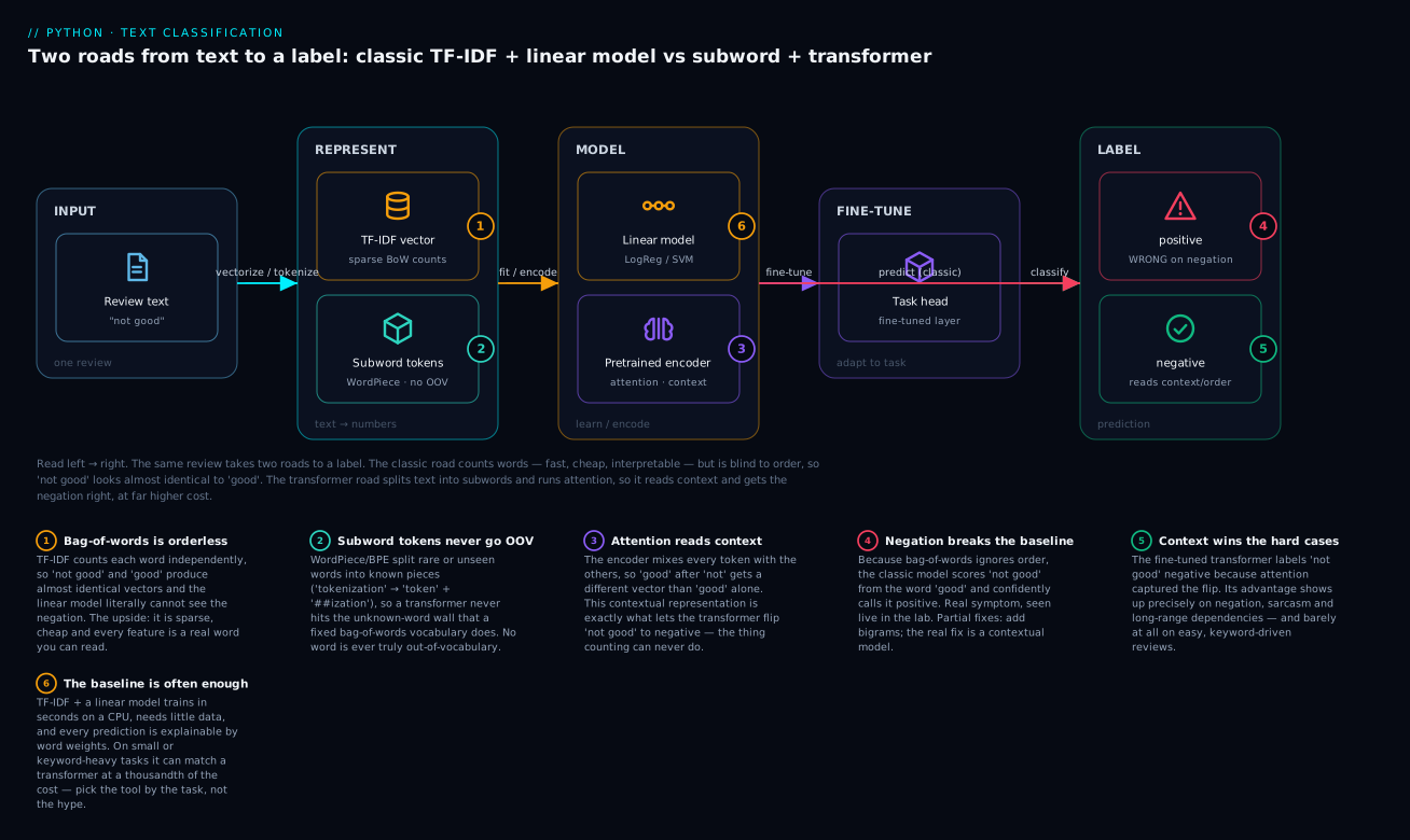
The six badges are the spine of the lesson. The classic path is orderless (1) and cheap and interpretable (6); the transformer path never hits an unknown word (2) and uses attention to read context (3); on a negated sentence the baseline breaks (4) while the contextual model wins (5). We will build the amber lane first, prove badge 4 live, then earn the purple lane.
| Classic family (this lesson’s baseline) | Transformer family | |
|---|---|---|
| Represents a word as | a fixed column in a sparse vector | a contextual dense vector, recomputed per sentence |
| Built by | counting (TF-IDF) | pretraining on huge text, then fine-tuning |
| Sees word order? | No (bag of words) | Yes (attention over positions) |
| Unknown words | become nothing (out-of-vocabulary) | split into known subword pieces — never OOV |
| Training cost | milliseconds, CPU | minutes–hours, usually a GPU |
| Interpretable? | Yes — read the coefficients | No — millions of opaque weights |
| Canonical tools | scikit-learn TfidfVectorizer + linear model |
Hugging Face transformers |
| Reaches (this lab) | 0.924 accuracy, misses negation | 1.000 on the same hard cases |
The classic baseline: TF-IDF + a linear classifier
The classical recipe is three components you already half-know: a TfidfVectorizer (Part 1) to make the features, a linear classifier to draw the decision boundary, and a Pipeline to bind them so no test information ever leaks into training. Let us build each piece, then fit it for real.
The whole model is one Pipeline
The single most important structural decision is to put the vectorizer and the classifier in one Pipeline. It is tempting to vectorize the whole corpus once and then split into train and test — and it is a silent, accuracy-inflating bug. TfidfVectorizer.fit learns the vocabulary and the IDF weights (how rare each word is). If it sees the test documents during fit, those IDF statistics are computed partly from data the model is about to be evaluated on. That is data leakage: the score you measure is optimistic, and it evaporates in production. This is the same leakage-safe discipline the scikit-learn Pipeline lesson drills — the vectorizer is a transformer with a fit/transform contract, exactly like a scaler.
from sklearn.pipeline import Pipeline
from sklearn.feature_extraction.text import TfidfVectorizer
from sklearn.linear_model import LogisticRegression

clf = Pipeline([
    ("tfidf", TfidfVectorizer()),
    ("lr", LogisticRegression(max_iter=1000, C=10)),
])
Now clf.fit(X_train, y_train) fits the vectorizer on the training text only, transforms it, and fits the classifier — all in the right order. And crucially, when you cross-validate, the vectorizer is re-fit inside every fold, so the IDF weights never see held-out data. The Pipeline is not a convenience; it is the thing that makes your evaluation honest.
| Wrong (leaks) | Right (Pipeline) |
|---|---|
X = Tfidf().fit_transform(all_text) then split |
split first, or let the Pipeline split inside CV |
| IDF learned from train and test | IDF learned from train only, per fold |
| Optimistic score, worse in production | Score you can trust |
Which linear classifier?
“Linear classifier” is a family, not one algorithm. On sparse, high-dimensional text vectors, three are the standard choices, and they are all linear — they draw a flat decision boundary and assign a weight to each word. That linearity is exactly what makes them fast and interpretable on 50,000-dimensional inputs where fancier models overfit or crawl. The deeper theory of these estimators is in the linear models, SVM, trees and kNN lesson; here is the text-specific summary.
| Classifier | scikit-learn class | Gives probabilities? | Strengths on text | Watch out |
|---|---|---|---|---|
| Logistic Regression | LogisticRegression |
✅ predict_proba |
Calibrated, interpretable coefficients, the default | Tune C (regularization) |
| Linear SVM | LinearSVC |
❌ (only decision_function) |
Often top accuracy on TF-IDF, fast | No probabilities; wrap in CalibratedClassifierCV if you need them |
| Multinomial Naive Bayes | MultinomialNB |
✅ | Blazing fast, a superb first baseline, loves counts | Assumes word independence; use CountVectorizer or TF-IDF |
| SGD (log/hinge loss) | SGDClassifier |
with log_loss |
Scales to millions of docs, online learning | More knobs to tune |
The honest default is LogisticRegression: it gives you calibrated probabilities (useful for thresholds and confidence), its coefficients are directly readable as per-word sentiment, and it is hard to beat on TF-IDF features. LinearSVC frequently edges it on raw accuracy but returns no probabilities. MultinomialNB is the fastest thing that works and a great sanity-check baseline. We use Logistic Regression for its interpretability — we are going to read what it learned.
One knob matters: C, the inverse of regularization strength. Small C (strong regularization) shrinks coefficients toward zero and under-fits; large C trusts the training data more. On a tiny corpus the default C=1.0 under-fits, so we set C=10, a value cross-validation confirms below. On a large corpus you would tune C with a grid search inside cross-validation.
Evaluating honestly: cross-validation, not a lucky split
We have a small, balanced dataset — 170 hand-labelled reviews, 85 positive and 85 negative (built in full in the lab). Here is a subtle, important thing that ties straight to the train/test split and metrics lesson: on 170 rows, a single train/test split is too noisy to trust. A 20-row test set can swing ten points of accuracy on the luck of which reviews land in it. The fix is k-fold cross-validation: split the data into k parts, train on k−1 and test on the held-out part, rotate, average. Every row is a test row exactly once, and the mean is a stable estimate.
from sklearn.model_selection import cross_val_score, cross_val_predict, StratifiedKFold
from sklearn.metrics import confusion_matrix, classification_report

cv = StratifiedKFold(n_splits=5, shuffle=True, random_state=0)
scores = cross_val_score(clf, texts, labels, cv=cv)
print("per-fold accuracy:", [round(float(s), 3) for s in scores])
print("mean CV accuracy:", round(float(scores.mean()), 3), "+/-", round(float(scores.std()), 3))
per-fold accuracy: [0.882, 0.912, 0.971, 0.971, 0.882]
mean CV accuracy: 0.924 +/- 0.04
92.4% ± 4%, and notice the per-fold spread (0.882 to 0.971) — that is the variance a single split would have hidden. StratifiedKFold keeps each fold balanced 50/50 so a fold can’t accidentally be all-positive; shuffle=True matters because our data is stored positives-then-negatives and unshuffled folds would be lopsided.
Accuracy alone lies on imbalanced data, so we look at the confusion matrix and per-class precision/recall. cross_val_predict gives an out-of-fold prediction for every row — leakage-safe, because each prediction comes from a model that never saw that row — so we can build one honest confusion matrix over all 170:
pred = cross_val_predict(clf, texts, labels, cv=cv)
print(confusion_matrix(labels, pred))
print(classification_report(labels, pred, target_names=["negative", "positive"], digits=3))
[[77  8]
 [ 5 80]]
              precision    recall  f1-score   support

    negative      0.939     0.906     0.922        85
    positive      0.909     0.941     0.925        85

    accuracy                          0.924       170
   macro avg      0.924     0.924     0.924       170
weighted avg      0.924     0.924     0.924       170
Read the matrix as [[TN FP] [FN TP]] with positive as the target class: 77 true negatives, 80 true positives, and only 8 + 5 = 13 errors out of 170. The classification report is the table you should quote to stakeholders, never a bare accuracy:
| Metric | Meaning for sentiment | This model |
|---|---|---|
| Precision (positive) | of reviews we called positive, how many were | 0.909 |
| Recall (positive) | of the actually positive reviews, how many we caught | 0.941 |
| F1 | harmonic mean of precision and recall | 0.925 |
| Support | how many true examples of the class | 85 |
| Macro avg | unweighted mean over classes (fair on imbalance) | 0.924 |
Why care about the split? Imagine a spam dataset that is 95% not-spam. A model that predicts “not-spam” every time scores 95% accuracy and is useless — its recall on spam is zero. Accuracy hides that; the confusion matrix and per-class recall expose it instantly. On our balanced set accuracy is fine, but the habit — always look at the matrix — is what keeps you from shipping a 95%-accurate model that never catches the thing you built it to catch.
Reading the model: coefficients are interpretability for free
This is the classic model’s superpower and the reason it refuses to die: you can read exactly what it learned. A linear model assigns one weight (coefficient) to each vocabulary word. Positive weight pushes toward the positive class, negative toward negative, and the magnitude is how strongly. Fit on the full data and sort:
clf.fit(texts, labels)
vocab = clf.named_steps["tfidf"].get_feature_names_out()
coefs = clf.named_steps["lr"].coef_[0]
order = coefs.argsort()
print("MOST POSITIVE:", [(vocab[i], round(float(coefs[i]), 2)) for i in order[-8:][::-1]])
print("MOST NEGATIVE:", [(vocab[i], round(float(coefs[i]), 2)) for i in order[:8]])
MOST POSITIVE: [('great', 4.7), ('best', 3.95), ('good', 3.75), ('excellent', 3.59), ('wonderful', 3.39), ('fantastic', 3.14), ('love', 2.88), ('superb', 2.84)]
MOST NEGATIVE: [('bad', -4.38), ('worst', -3.77), ('terrible', -3.71), ('poor', -3.51), ('awful', -3.39), ('dreadful', -2.83), ('hate', -2.82), ('horrible', -2.61)]
The model taught itself English sentiment vocabulary from 170 examples: great, best, good, excellent push positive; bad, worst, terrible, awful push negative. No transformer gives you this. When a linear model misclassifies, you can point at the words that did it; when a 67-million-parameter transformer misclassifies, you get a shrug. In regulated settings (credit, hiring, health) that auditability is not a nicety — it is a legal requirement, and it can be the deciding reason to ship the linear model.
When the baseline is genuinely the right tool
Do not read “baseline” as “the thing you replace.” For an enormous class of real problems, TF-IDF + a linear model is the production system, on purpose.
| Choose the classic baseline when… | Because |
|---|---|
| You have little labelled data (hundreds–thousands) | Linear models generalize from small data; transformers overfit it |
| Predictions must be explainable/auditable | Coefficients name the responsible words |
| Latency and cost are tight (high QPS, edge, CPU-only) | ~0.2 ms/prediction, no GPU, tiny memory |
| The signal is keyword-driven (spam, topic, tags) | Presence of words is enough; order barely matters |
| You need a baseline before anything fancy | It sets the bar every complex model must clear |
| The team must maintain it | pip install scikit-learn and 20 lines, no ML platform |
Build this first, always. It takes ten minutes, it tells you how hard your problem actually is, and often it is good enough to ship. Only when you can show its specific blindness is costing real accuracy do you pay for a transformer.
Where bag-of-words hits the wall
Our model scores 92.4%. Watch it fall on its face on the one thing sentiment most needs — negation. This is the demonstration the whole lesson pivots on.
print("'not' in vocabulary?", "not" in set(vocab))
v1 = clf.named_steps["tfidf"].transform(["this was good"])
v2 = clf.named_steps["tfidf"].transform(["this was not good"])
print("vectors identical?", (v1 != v2).nnz == 0)
for s in ["this was good", "this was not good", "i loved it", "i did not love it"]:
    prob = clf.predict_proba([s])[0][1]
    print(f"{s!r:22} -> {'positive' if prob >= .5 else 'negative'}  P(pos)={prob:.2f}")
'not' in vocabulary? False
vectors identical? True
'this was good'        -> positive  P(pos)=0.89
'this was not good'    -> positive  P(pos)=0.89
'i loved it'           -> positive  P(pos)=0.72
'i did not love it'    -> positive  P(pos)=0.91
Look at what just happened. "this was not good" and "this was good" produce the byte-for-byte identical feature vector (vectors identical? True), so the model gives them the identical prediction: both positive, both 0.89. The classifier cannot tell a good review from its exact negation. Two reasons stack up:
notis not in the vocabulary at all (False) — it never appeared in the 170 training reviews, so at prediction time the vectorizer silently drops it as an unknown word."this was not good"is represented as just{this, was, good}— literally the same as"this was good".- Even if
notwere in the vocabulary, it wouldn’t help. Bag of Words is orderless — it records that the wordsnotandgoodare present, but not thatnotcomes beforegoodand flips it.notwould be its own independent feature with its own weight, unable to modifygood.
And the punchline in the last line: "i did not love it" scores more positive (0.91) than "i loved it" (0.72), because love has a big positive coefficient (2.88) and the did not in front of it is invisible. Adding a negation made the model more confident of the opposite. This is not a bug in our code; it is the fundamental ceiling of counting words.
| Bag-of-words blind spot | Example | What the model sees |
|---|---|---|
| Word order | "dog bites man" vs "man bites dog" |
identical vectors |
| Negation | "not good" vs "good" |
not dropped or inert → same class |
| Long-range context | "the food, despite the reviews, was bad" |
just a bag of words, connection lost |
| Synonyms / meaning | "great" vs "superb" |
unrelated columns, zero similarity |
| Out-of-vocabulary words | a new slang word or brand | dropped entirely — no representation |
| Sarcasm | "oh brilliant, it broke again" |
brilliant pulls positive |
n-grams (Part 1’s ngram_range=(1,2)) patch the first two rows a little — a not good bigram becomes its own feature if it appeared in training — at the cost of a vocabulary explosion, and they do nothing for synonyms or genuine long-range context. To actually fix this you need a representation that (a) never runs out of vocabulary and (b) computes each word’s meaning from its neighbours. That is embeddings, then transformers.
From static to contextual embeddings
The synonym problem — great and superb being unrelated columns — is what word embeddings solved first (this is the bridge Part 1 ended on). Instead of one sparse column per word, represent each word as a dense vector of a few hundred learned numbers, trained so that words used in similar contexts get similar vectors. great and superb land close; cat and dog land close; and analogies become arithmetic: king − man + woman ≈ queen. Meaning becomes geometry.
But word2vec (2013) and GloVe (2014) embeddings are static: one fixed vector per word, computed once and frozen. And that is their ceiling. The word bank gets a single vector that must simultaneously mean river bank and savings bank; good gets one vector whether or not a not precedes it. Static embeddings fix synonyms but not context.
Contextual embeddings are the leap. A transformer produces a different vector for a word depending on the sentence it sits in. bank in “river bank” and bank in “bank robber” come out as different vectors; good in “very good” and good in “not good” come out different. The representation is computed fresh for every sentence, from the actual neighbours. That single change — from a frozen lookup table to a context-computed vector — is what lets a transformer read the negation our linear model was blind to.
| Sparse (TF-IDF) | Static embeddings (word2vec/GloVe) | Contextual (transformer) | |
|---|---|---|---|
| Vector per word | one column, mostly zeros | one dense vector, fixed | a dense vector per context |
good in “not good” |
same as “good” | same as “good” | different from “good” |
| Captures synonyms? | No | Yes | Yes |
| Captures negation/order? | No | No | Yes |
| Dimensions | 10k–100k | 50–300 | 256–1024 |
| Made by | counting | shallow net over co-occurrence | deep transformer, pretrained |
The transformer, intuitively
A transformer is, underneath, a deep neural network — so if the intuition of layers, weights and gradient-descent training is fresh, you already have the scaffolding, and attention is simply one particular kind of layer stacked many times. You do not need the matrix algebra to use transformers well; you need four ideas. Here they are, in plain terms.
1. Attention — “which other words matter for this one”
The engine of a transformer is self-attention. For every word, the model asks: to compute my meaning here, which other words in this sentence should I look at, and how much? It then builds each word’s vector as a weighted blend of the others. For good in "not good", attention learns to look hard at not, and the resulting vector for good is pulled toward “negated.” Picture it as a small table of weights: when the model builds the vector for good, it might place most of its attention on not and the rest on itself, so “negated” is literally mixed into good’s representation before the classifier ever sees it. Stack a dozen such attention layers and the model composes meaning from ever-wider context. That is, mechanically, how the model sees negation: the representation of good is computed from not. No counting scheme can do this, because counting throws the neighbours away.
Attention is also all-to-all and order-aware: every word can attend to every other, near or far, so “the food, despite the glowing reviews, was bad” connects bad to food across the whole clause. Position information is injected too (positional encodings), so "man bites dog" and "dog bites man" are genuinely different inputs — unlike Bag of Words, where they were identical.
2. Subword tokenization — why models never see an unknown word
Recall the classic model dropped not because it was out-of-vocabulary. Transformers make OOV impossible by tokenizing into subwords. A fixed vocabulary of ~30,000 frequent character-chunks is learned; any word is spelled out of those pieces. Real output from the DistilBERT tokenizer we ran:
from transformers import AutoTokenizer
tok = AutoTokenizer.from_pretrained("distilbert-base-uncased")
for w in ["tokenization", "antidisestablishmentarianism", "kloudvin"]:
    print(f"{w!r:32} -> {tok.tokenize(w)}")
'tokenization'                   -> ['token', '##ization']
'antidisestablishmentarianism'   -> ['anti', '##dis', '##est', '##ab', '##lish', '##ment', '##arian', '##ism']
'kloudvin'                       -> ['k', '##lou', '##d', '##vin']
tokenization becomes token + ##ization (the ## means “continues the previous token”). A monster word decomposes into eight familiar pieces. Even kloudvin — a made-up word the model has never seen — is spelled out as k + ##lou + ##d + ##vin rather than thrown away. No word is ever truly out-of-vocabulary, which is exactly the wall our TF-IDF model hit. The common schemes:
| Scheme | Used by | Idea |
|---|---|---|
| BPE (byte-pair encoding) | GPT, RoBERTa | merge the most frequent character pairs, greedily |
| WordPiece | BERT, DistilBERT | like BPE, merges by likelihood; ## marks continuations |
| SentencePiece / Unigram | T5, LLaMA, multilingual | language-agnostic, works on raw bytes, no pre-tokenization |
3. Pretraining then fine-tuning — learn language once, adapt cheaply
A transformer is trained in two phases. Pretraining runs on a gigantic pile of raw text (much of the web) with a self-supervised objective that needs no labels — so it can use all the text in the world. Fine-tuning then takes that language-savvy model and nudges it on your small labelled task (a few thousand sentiment reviews) for a few minutes. The heavy lifting — learning what English is — happened once, at someone else’s expense; you inherit it and adapt. This is why a transformer can beat a from-scratch model on tiny labelled data: it did not start from zero.
| Pretraining objective | Family | What it learns |
|---|---|---|
| Masked language modelling (fill the blank) | encoders (BERT) | deep bidirectional understanding |
| Causal / next-token (predict the next word) | decoders (GPT) | fluent generation |
| Span corruption / denoising | seq2seq (T5, BART) | rewrite input into output |
4. Three architecture families
“Transformer” splits into three shapes, and which one you want depends on the task.
| Family | Reads | Canonical models | Best at | Our task? |
|---|---|---|---|---|
| Encoder | whole input at once, bidirectionally | BERT, RoBERTa, DistilBERT | classification, NER, embeddings | ✅ this is what we use |
| Decoder | left to right, generates | GPT, LLaMA, Mistral | text generation, chat, LLMs | overkill for a label |
| Encoder–decoder (seq2seq) | reads then writes | T5, BART | translation, summarization | for input→output text |
For classification, you want an encoder — it reads the entire review bidirectionally and hands a single sentence vector to a small classifier head. That is precisely what distilbert-base-uncased-finetuned-sst-2-english is: DistilBERT (an encoder) with a sentiment head fine-tuned on the SST-2 movie-review dataset. Large Language Models (GPT-4, Claude, LLaMA) are the decoder family scaled to billions of parameters; they can also classify — you just ask them in a prompt — but using a 100-billion-parameter chat model to label a review positive/negative is using a wrecking ball to hang a picture. Match the family to the job.
The Hugging Face ecosystem
Hugging Face transformers is the library that made all of this a few lines of Python. It is the npm of NLP models: a hub of hundreds of thousands of pretrained models and a uniform API to run them.
pipeline() — zero-code inference
The fastest path from “installed” to “running a transformer” is pipeline(). Name a task; it downloads a sensible default model and gives you a callable. We ran this for real on the same sentences that broke the classic model:
from transformers import pipeline
clf = pipeline("sentiment-analysis")   # defaults to distilbert SST-2, ~268 MB

for s in ["this was good", "this was not good", "i loved it",
          "i did not love it", "not bad at all",
          "the acting was good but the plot was terrible"]:
    r = clf(s)[0]
    print(f"{s!r:48} -> {r['label']:8} ({r['score']:.3f})")
'this was good'                                  -> POSITIVE (1.000)
'this was not good'                              -> NEGATIVE (1.000)
'i loved it'                                     -> POSITIVE (1.000)
'i did not love it'                              -> NEGATIVE (0.999)
'not bad at all'                                 -> POSITIVE (0.999)
'the acting was good but the plot was terrible'  -> NEGATIVE (0.998)
This is real output, and it is the payoff. Line by line the transformer gets right everything the classic model got wrong. "this was not good" → NEGATIVE (1.000) — where our linear model said positive 0.89. "i did not love it" → NEGATIVE (0.999) — where the linear model said positive 0.91. It even nails "not bad at all" (a double negative, so positive) and reads the contrastive "good ... but ... terrible" as negative. Attention did that: the vector for good in "not good" was computed from not, so the flip is baked into the representation.
⚠️ The first
pipeline(...)call downloads a model (here ~268 MB) from the internet to a local cache (~/.cache/huggingface). Subsequent runs are offline and instant. On a metered or firewalled machine, know that a several-hundred-MB download is about to happen.
pipeline is not just sentiment. The same three-line pattern runs a dozen tasks, each defaulting to an appropriate model:
pipeline(task=...) |
Does | Default model family |
|---|---|---|
"sentiment-analysis" |
positive/negative (what we ran) | DistilBERT (encoder) |
"text-classification" |
any labelled classification | encoder |
"ner" / "token-classification" |
tag people, orgs, places | encoder |
"zero-shot-classification" |
classify into your labels, no training | NLI encoder |
"summarization" |
shorten text | BART/T5 (seq2seq) |
"translation_xx_to_yy" |
translate | seq2seq |
"question-answering" |
answer from a context passage | encoder |
"fill-mask" |
fill a [MASK] |
encoder |
"text-generation" |
continue a prompt | decoder (GPT-family) |
Honesty note on what executed. The
sentiment-analysispipeline and the tokenizer output above are real — that model downloaded and ran on this machine. The other tasks in the table each pull their own (often larger, 1 GB+) model; to keep the lab lean I did not download those, so I describe them rather than paste fabricated output. The API shape is identical —pipeline("ner")("Apple is in California")returns a list of{entity_group, word, score}dicts — but I will not invent numbers I did not run.
Which model? pipeline picks a default, but you should usually name one with model=, and size is the main lever. Our model is DistilBERT — a distilled version of BERT: a smaller student network trained to mimic the larger teacher, ending up roughly 40% smaller and 60% faster while keeping about 97% of BERT’s accuracy. Distilled models (distilbert-...) and tiny ones (prajjwal1/bert-tiny, a few MB) are the right default when latency, memory or download size matters — which, in production, is almost always. Reach for a full-size model (bert-large, roberta-large) only when the accuracy gain is measured and needed. The Hugging Face Hub lists each model’s size and task, so you pick with eyes open rather than accepting whatever the default pulls.
AutoTokenizer and AutoModel — one layer down
pipeline is the front door. One level down, the Auto* classes let you drive the tokenizer and model directly — needed for batching, custom heads, or fine-tuning. The tokenizer turns text into the integer IDs the model eats; here is the real encoding of our problem sentence:
from transformers import AutoTokenizer
tok = AutoTokenizer.from_pretrained("distilbert-base-uncased-finetuned-sst-2-english")
enc = tok("this was not good", return_tensors="pt")
print("input_ids:", enc["input_ids"].tolist())
print("tokens   :", tok.convert_ids_to_tokens(enc["input_ids"][0].tolist()))
input_ids: [[101, 2023, 2001, 2025, 2204, 102]]
tokens   : ['[CLS]', 'this', 'was', 'not', 'good', '[SEP]']
Here is the contrast made concrete: the transformer tokenizes not as ID 2025 and keeps it — a real token attention can act on — whereas our TF-IDF model dropped the same word. The tokenizer also adds special tokens: [CLS] (ID 101) at the front, whose final vector is the sentence summary the classifier head reads, and [SEP] (ID 102) at the end. The matching pattern for classification is AutoModelForSequenceClassification:
| Auto class | Loads a model for |
|---|---|
AutoTokenizer |
text ↔ token IDs (always pair with the model) |
AutoModel |
raw hidden-state vectors (embeddings) |
AutoModelForSequenceClassification |
classification (sentiment, NLI) |
AutoModelForTokenClassification |
NER, POS tagging |
AutoModelForQuestionAnswering |
extractive QA |
AutoModelForCausalLM |
text generation (GPT-family) |
AutoModelForSeq2SeqLM |
translation, summarization |
The model exposes its label map and size, which you should always check — the real values for our model:
labels: {0: 'NEGATIVE', 1: 'POSITIVE'} | params: 67M | model_max_length: 512
pipeline device: mps:0 | model dtype: torch.float32
Two things worth reading there. model_max_length: 512 — DistilBERT accepts at most 512 tokens; longer text is truncated (more in troubleshooting). And device: mps:0 — on this Apple-Silicon Mac, transformers auto-selected the Metal (MPS) GPU backend; on a CPU-only box it would read cpu and run several times slower. Batched inference measured ~10 ms per text on MPS here — versus 0.2 ms for the linear model on CPU. That 50× latency gap, times your request volume, is a real line in the decision below.
Fine-tuning — adapting a pretrained model to your task
pipeline runs a model someone already fine-tuned. When your task is not a standard one, you fine-tune your own: take a pretrained encoder, attach a fresh classification head, and train briefly on your labelled data. The Trainer API is the standard harness. The sketch below is illustrative — it is not executed in this lesson (fine-tuning needs a labelled dataset and minutes of GPU time), but it is the real shape:
# SKETCH — not run here. The real fine-tuning loop, conceptually.
from transformers import (AutoTokenizer, AutoModelForSequenceClassification,
                          TrainingArguments, Trainer)

tok = AutoTokenizer.from_pretrained("distilbert-base-uncased")
model = AutoModelForSequenceClassification.from_pretrained(
    "distilbert-base-uncased", num_labels=2)          # fresh 2-class head

def encode(batch):
    return tok(batch["text"], truncation=True, padding="max_length", max_length=128)

# ds = load_dataset(...).map(encode, batched=True)     # your labelled data
args = TrainingArguments(output_dir="out", num_train_epochs=3,
                         per_device_train_batch_size=16, learning_rate=2e-5)
trainer = Trainer(model=model, args=args,
                  train_dataset=ds["train"], eval_dataset=ds["test"])
# trainer.train()                                       # minutes on a GPU
The mental model: from_pretrained("distilbert-base-uncased", num_labels=2) loads the language-savvy body and bolts on an untrained 2-class head; Trainer.train() nudges the whole thing on your labels with a tiny learning rate (2e-5 — small, so you adapt rather than clobber what pretraining learned). Three epochs on a few thousand examples is typical. Exact TrainingArguments fields drift between library versions, so check the docs for your transformers — the idea (pretrained body + new head + gentle training) is stable.
There are three ways to use a pretrained model, in ascending cost and power:
| Approach | What you do | Cost | When |
|---|---|---|---|
| Feature extraction | freeze the model, use its vectors as features for a linear head | low | little data, fast iteration |
| Fine-tuning | update the model’s weights on your labels | medium (GPU, minutes–hours) | you have labels and want top accuracy |
| Prompting (LLM) | ask a big generative model in words, no training | zero training, per-call cost | no labels, or fast prototyping |
TF-IDF + linear vs a transformer: the honest decision
Here is the table the hype skips. A transformer is not always the right answer. Decide by your constraints, not by what is fashionable.
| Dimension | TF-IDF + linear | Transformer (fine-tuned) | Winner |
|---|---|---|---|
| Labelled data needed | hundreds | thousands+ (or pretrained) | classic on tiny data |
| Accuracy on easy/keyword tasks | high | marginally higher | ~tie (classic cheaper) |
| Accuracy on negation/context/sarcasm | poor | strong | transformer |
| Training cost | ~2 ms, CPU | minutes–hours, GPU | classic |
| Inference latency | ~0.2 ms/text, CPU | ~10 ms/text, GPU/MPS | classic (≈50×) |
| Model size | kilobytes | hundreds of MB–GB | classic |
| Interpretability | full (read coefficients) | near zero | classic |
| Handles new/OOV words | drops them | subword — never OOV | transformer |
| Ops complexity | pip install scikit-learn |
GPU, model serving, caching | classic |
The engineering summary: build the classic baseline first, every time. It is ten minutes of work, it quantifies how hard your problem is, and for keyword-driven tasks with tight latency it is the final answer. Reach for a transformer when you can demonstrate the baseline’s blindness — negation, context, sarcasm, rare vocabulary — is costing accuracy you need, and you can afford the GPU, the size, and the loss of interpretability. Our own lab is the microcosm: on the balanced, keyword-heavy reviews the linear model scored 92.4%; on the negation sentences it scored 0%. If your real traffic looks like the former, ship the linear model. If it looks like the latter, pay for the transformer.
Where the field is going (briefly)
The frontier moved past fine-tuning small encoders, though everything above is still the right tool for most classification. Three shifts worth naming:
- LLMs as zero-shot classifiers. Instead of fine-tuning, you can prompt a large decoder (“Classify the sentiment as positive or negative: …”) and get a label with no training data. Fast to prototype, but slower, costlier per call, and less controllable than a fine-tuned encoder. Great when you have no labels; wasteful at high volume when you do.
- Prompt vs fine-tune. The real trade: prompting needs zero labelled data and zero training but pays per inference and is harder to pin down; fine-tuning needs labels and a training run but yields a small, fast, consistent, cheap-to-serve model. High volume + labels → fine-tune. Low volume or no labels → prompt.
- RAG (retrieval-augmented generation). For tasks that need facts the model was not trained on, RAG retrieves relevant documents (often via the embeddings this lesson introduced) and feeds them into an LLM’s prompt. Notice the through-line: the TF-IDF-and-cosine-similarity search from Part 1 is the ancestor of the dense-vector retrieval powering modern RAG. The pipeline you learned did not get replaced — it got a better representation.
| Approach | Labels? | Training? | Per-call cost | Best for |
|---|---|---|---|---|
| TF-IDF + linear | yes (few) | seconds | ~nothing | cheap, interpretable, keyword tasks |
| Fine-tuned encoder | yes | minutes–hours | low | high-volume classification, top accuracy |
| LLM prompting (zero-shot) | no | none | high | no labels, prototyping, flexible tasks |
| RAG | no (for the LLM) | none–some | high | answers grounded in your documents |
Hands-on lab
Build both classifiers end to end and watch the transformer fix the exact failure of the baseline. The classic half runs anywhere; the transformer half needs the model download.
⚠️ This lab installs packages and (in Step 5) downloads a ~268 MB model. Use a virtual environment so nothing touches system Python.
Step 1 — Environment.
mkdir -p ~/pylab/nlp2 && cd ~/pylab/nlp2
python3.12 -m venv .venv
source .venv/bin/activate           # Windows: .venv\Scripts\activate
python -m pip install --upgrade pip
pip install scikit-learn            # the classic half — runs for sure
Step 2 — Build the labelled dataset. Save as sentiment.py. It is 85 positive and 85 negative short reviews. (Deliberately, the word not never appears in training — that is what makes the negation failure so clean.)
positive = [
    "I loved this movie, it was absolutely fantastic", "An amazing film with a brilliant story",
    "Wonderful acting and a great script", "This is the best product I have ever bought",
    "Excellent quality and superb value for money", "A perfect experience, I highly recommend it",
    "The food was delicious and the service was great", "I am so happy with this purchase",
    "Beautiful design and it works flawlessly", "Truly enjoyable, a delightful and charming story",
    "Fantastic value, I would buy it again", "The staff were friendly and helpful",
    "A wonderful, heartwarming and inspiring film", "Superb performance and well worth the price",
    "Great battery life and a gorgeous screen", "I really love how easy it is to use",
    "Outstanding quality that exceeded my expectations", "A brilliant and memorable experience",
    "The best meal I have had in years", "Highly satisfied, everything was perfect",
    "This product is good and reliable", "A good movie with good acting",
    "Good value and good quality overall", "The service was good and very fast",
    "Such a good and enjoyable read", "I love it, the design is excellent",
    "Great phone with an amazing camera", "The hotel was clean and the staff were great",
    "An excellent purchase, I am delighted", "Fantastic customer support, very helpful",
    "The best coffee in town, I absolutely love it", "A great little gadget that works perfectly",
    "Loved every minute, a wonderful show", "Amazing flavour and generous portions",
    "This laptop is fast and beautifully built", "A superb hotel with a lovely view",
    "Really good, I would recommend it to a friend", "Excellent value and speedy delivery",
    "The book was engaging and brilliantly written", "Perfect fit and great comfortable material",
    "A joy to use, intuitive and reliable", "Wonderful holiday, we had a great time",
    "The best decision I made this year", "Superb quality and a fair price",
    "I am impressed, it works great", "A lovely, warm and friendly restaurant",
    "Great sound and excellent build quality", "This is a good, solid and dependable car",
    "Delicious meal and a pleasant atmosphere", "Absolutely brilliant, I love this app",
    "Great product, I highly recommend it", "Excellent service and fast delivery",
    "Love it, works perfectly every time", "Fantastic quality for the price",
    "The best purchase I have made", "Amazing product, absolutely love it",
    "Wonderful experience from start to finish", "Perfect, exactly what I wanted",
    "Brilliant value, very happy with it", "Good product and great support",
    "Really happy, it works great", "Excellent, would definitely buy again",
    "Superb quality, highly recommend it", "A great deal and a lovely product",
    "Love this, it is fantastic", "Good quality and a great price",
    "The best, I am very satisfied", "Amazing value and wonderful design",
    "Perfect product, works like a charm", "Great experience, friendly and helpful staff",
    "Excellent build and a beautiful finish", "Very good, I am delighted with it",
    "Fantastic, everything works perfectly", "Wonderful product, exceeded my expectations",
    "Highly recommend, great value for money", "Love the design, it is excellent",
    "Best decision ever, so happy with it", "Great little product, works well",
    "Superb service and a perfect result", "Amazing quality, I am impressed",
    "Good value, would recommend to anyone", "Excellent product and speedy shipping",
    "Really great, I love using it", "Perfect fit and great quality",
    "Wonderful, a truly delightful product",
]
negative = [
    "I hated this movie, it was a total waste of time", "A terrible film with a boring plot",
    "Awful acting and a dreadful script", "This is the worst product I have ever bought",
    "Poor quality and a complete rip-off", "A horrible experience that I deeply regret",
    "The food was cold and the service was slow", "I am so disappointed with this purchase",
    "Cheap design and it broke on the first day", "Utterly boring, a dull and tedious story",
    "Terrible value, I want a refund", "The staff were rude and unhelpful",
    "A dreadful, depressing and pointless film", "Weak performance and nowhere near worth the price",
    "Awful battery life and a cracked screen", "I really hate how confusing it is to use",
    "Disappointing quality, far below my expectations", "A forgettable and frustrating experience",
    "The worst meal I have had in years", "Deeply unsatisfied, everything was wrong",
    "This product is bad and unreliable", "A bad movie with bad acting",
    "Bad value and bad quality overall", "The service was bad and very slow",
    "Such a bad and tedious read", "I hate it, the design is terrible",
    "Terrible phone with an awful camera", "The hotel was dirty and the staff were rude",
    "An awful purchase, I am furious", "Terrible customer support, totally useless",
    "The worst coffee in town, I hate it", "A useless gadget that broke immediately",
    "Hated every minute, a dreadful show", "Bland flavour and tiny portions",
    "This laptop is slow and cheaply built", "A horrible hotel with a depressing view",
    "Really bad, I would avoid it entirely", "Poor value and painfully slow delivery",
    "The book was dull and badly written", "Poor fit and cheap uncomfortable material",
    "A pain to use, clunky and unreliable", "Awful holiday, we had a terrible time",
    "The worst decision I made this year", "Poor quality and an unfair price",
    "I am annoyed, it barely works", "A cold, unwelcoming and rude restaurant",
    "Bad sound and poor build quality", "This is a bad, flimsy and unreliable car",
    "Disgusting meal and an unpleasant atmosphere", "Absolutely terrible, I hate this app",
    "Terrible product, I regret buying it", "Awful service and slow delivery",
    "Hate it, breaks all the time", "Poor quality for the price",
    "The worst purchase I have made", "Terrible product, absolutely hate it",
    "Horrible experience from start to finish", "Useless, a complete waste of money",
    "Bad value, very unhappy with it", "Poor product and terrible support",
    "Really unhappy, it barely works", "Awful, would never buy again",
    "Terrible quality, avoid at all costs", "A bad deal and a cheap product",
    "Hate this, it is dreadful", "Bad quality and a high price",
    "The worst, I am very dissatisfied", "Awful value and horrible design",
    "Terrible product, broke straight away", "Bad experience, rude and unhelpful staff",
    "Poor build and an ugly finish", "Very bad, I am disgusted with it",
    "Dreadful, nothing works properly", "Horrible product, far below my expectations",
    "Would avoid, poor value for money", "Hate the design, it is awful",
    "Worst decision ever, so unhappy with it", "Terrible little product, works badly",
    "Poor service and a dreadful result", "Awful quality, I am furious",
    "Bad value, a real disappointment for anyone", "Terrible product and painfully slow shipping",
    "Really bad, I hate using it", "Poor fit and bad quality",
    "Dreadful, a truly disappointing product",
]
texts = positive + negative
labels = [1] * len(positive) + [0] * len(negative)
What just happened: a balanced 170-row corpus, positive labelled 1 and negative 0 — enough signal for a real classifier, small enough to run instantly.
Step 3 — Train and evaluate the classic model. Append:
from sklearn.pipeline import Pipeline
from sklearn.feature_extraction.text import TfidfVectorizer
from sklearn.linear_model import LogisticRegression
from sklearn.model_selection import cross_val_score, cross_val_predict, StratifiedKFold
from sklearn.metrics import confusion_matrix, classification_report

clf = Pipeline([("tfidf", TfidfVectorizer()),
                ("lr", LogisticRegression(max_iter=1000, C=10))])
cv = StratifiedKFold(n_splits=5, shuffle=True, random_state=0)
print("mean CV accuracy:", round(float(cross_val_score(clf, texts, labels, cv=cv).mean()), 3))
pred = cross_val_predict(clf, texts, labels, cv=cv)
print(confusion_matrix(labels, pred))
print(classification_report(labels, pred, target_names=["negative", "positive"], digits=3))
mean CV accuracy: 0.924
[[77  8]
 [ 5 80]]
              precision    recall  f1-score   support
    negative      0.939     0.906     0.922        85
    positive      0.909     0.941     0.925        85
    accuracy                          0.924       170
What just happened: a leakage-safe Pipeline, evaluated by 5-fold cross-validation (honest on small data). 92.4% accuracy, only 13 errors out of 170.
Step 4 — Read the coefficients, then break it on negation. Append:
clf.fit(texts, labels)
vocab = clf.named_steps["tfidf"].get_feature_names_out()
coefs = clf.named_steps["lr"].coef_[0]
order = coefs.argsort()
print("POS:", [vocab[i] for i in order[-6:][::-1]])
print("NEG:", [vocab[i] for i in order[:6]])
print("'not' in vocab?", "not" in set(vocab))
for s in ["this was good", "this was not good", "i did not love it"]:
    print(f"{s!r:22} P(pos)={clf.predict_proba([s])[0][1]:.2f}")
POS: ['great', 'best', 'good', 'excellent', 'wonderful', 'fantastic']
NEG: ['bad', 'worst', 'terrible', 'poor', 'awful', 'dreadful']
'not' in vocab? False
'this was good'        P(pos)=0.89
'this was not good'    P(pos)=0.89
'i did not love it'    P(pos)=0.91
What just happened: the model learned real sentiment words (fully interpretable) — and then failed exactly as predicted. not is not in the vocabulary, so "this was not good" scores identically to "this was good" (both 0.89 positive), and "i did not love it" is more positive than the plain review. Bag of Words is blind to negation.
Step 5 — The transformer on the same sentences. Install the transformer stack. The brief’s suggested --index-url https://download.pytorch.org/whl/cpu works on Linux/Windows; on macOS, PyPI’s torch is already CPU/MPS, so plain pip install is correct:
pip install torch transformers          # macOS: PyPI wheels are CPU/MPS
# Linux/Windows CPU-only alternative:
# pip install transformers && pip install torch --index-url https://download.pytorch.org/whl/cpu
Save as transformer_demo.py:
from transformers import pipeline
clf = pipeline("sentiment-analysis")    # downloads distilbert SST-2 (~268 MB) on first run
for s in ["this was good", "this was not good", "i did not love it",
          "not bad at all", "the acting was good but the plot was terrible"]:
    r = clf(s)[0]
    print(f"{s!r:48} -> {r['label']:8} ({r['score']:.3f})")
'this was good'                                  -> POSITIVE (1.000)
'this was not good'                              -> NEGATIVE (1.000)
'i did not love it'                              -> NEGATIVE (0.999)
'not bad at all'                                 -> POSITIVE (0.999)
'the acting was good but the plot was terrible'  -> NEGATIVE (0.998)
What just happened: the real transformer, run locally, fixed every failure. "this was not good" → NEGATIVE, "i did not love it" → NEGATIVE, and even the double-negative "not bad at all" → POSITIVE. Attention computed the meaning of each word from its neighbours, so negation flipped the label — the thing counting words can never do. Same five sentences; the classic model called the first three positive, the transformer got all five right.
You have now built both families, measured the baseline honestly, proven its blind spot, and watched a contextual model close it — the whole arc of modern text classification in one directory.
Common mistakes and troubleshooting
| Symptom / traceback | Cause | Fix |
|---|---|---|
Sentiment model calls "not good" positive |
Bag of Words ignores word order; not inert or dropped |
Add ngram_range=(1,2), or use a transformer for negation-heavy text |
| CV accuracy far above the held-out score | TfidfVectorizer.fit saw test data (leakage) |
Put vectorizer + classifier in one Pipeline; fit inside each fold |
| 97% accuracy but it never catches the rare class | Imbalanced data; accuracy is fooled | Read the confusion matrix; report per-class precision/recall, use class_weight="balanced" |
| Accuracy swings 10 pts between runs | Tiny test split, high variance | Use cross_val_score / StratifiedKFold, not one split |
| Transformer overfits / underperforms on 200 rows | Too little data for millions of params | Use TF-IDF + linear on small data; fine-tune only with thousands of labels |
OSError: Can't load ... / connection error |
Model download failed (offline, firewall, HF down) | Retry; pre-download to ~/.cache/huggingface; set HF_HOME; check proxy |
| Model download is gigabytes / too slow | Default model for the task is large | Pick a small model explicitly (distilbert-..., prajjwal1/bert-tiny) |
Token indices sequence length is longer than 512 |
Input exceeds the model’s max length | tokenizer(text, truncation=True, max_length=512) — or the tail is silently cut |
| Transformer inference painfully slow | Big model on CPU, no batching | Batch inputs; use a smaller/distilled model; move to GPU/MPS with device= |
ValueError: could not convert string to array |
Fed raw text to an estimator expecting numbers | Vectorize first (the whole point of the Pipeline) |
.similarity warns / a static vector for bank never changes |
Treating a static embedding as contextual | Static = one vector per word; use a transformer for context |
| Prompting an LLM per row is expensive and slow | Using a decoder LLM where a fine-tuned encoder fits | Fine-tune a small encoder for high-volume classification |
LinearSVC has no predict_proba |
SVMs give margins, not probabilities | Use LogisticRegression, or wrap in CalibratedClassifierCV |
Three that bite hardest, in prose:
1. Leakage is the silent accuracy inflater. If you call TfidfVectorizer().fit_transform(all_documents) and then split into train and test, the IDF weights and vocabulary were computed using the test set. Your cross-validation score comes out flattering and collapses in production. The whole reason to wrap the vectorizer and classifier in a single Pipeline is that cross-validation then re-fits the vectorizer inside each fold, on training data only. Leakage produces no error and no warning — just a number you should not have trusted. Pipeline-everything is the discipline that prevents it.
2. Accuracy is a liar on imbalanced data. A model on a 95%-negative dataset can score 95% by always predicting negative, while catching zero positives. This is the single most common way a text classifier looks great in a notebook and is useless in production. Never report accuracy alone: report the confusion matrix and per-class recall, and when a class is rare, weight it (class_weight="balanced") or resample. Our balanced lab hides this, but the habit — always look at the matrix — is what saves you on the imbalanced problems you will actually meet.
3. A transformer on tiny data is the wrong reflex. Fine-tuning a 67-million-parameter model on 200 labelled reviews overfits: it memorizes rather than generalizes, and a linear model on TF-IDF beats it while training in milliseconds and staying interpretable. The transformer’s edge appears when you have enough labels and the task genuinely needs context (negation, sarcasm, long-range dependencies). Reaching for the big model first — before you have measured the cheap baseline — costs you time, money, and interpretability for often no accuracy gain. Baseline first, always; upgrade only on evidence.
Cheat-sheet
Classic pipeline (scikit-learn)
| Call | Does |
|---|---|
Pipeline([("tfidf", TfidfVectorizer()), ("clf", LogisticRegression())]) |
leakage-safe vectorize + classify |
clf.fit(X_train, y_train) |
fit vectorizer on train, then classifier |
TfidfVectorizer(ngram_range=(1,2), min_df=2, stop_words="english") |
common production knobs |
LogisticRegression(C=10, max_iter=1000) |
linear classifier; C = inverse regularization |
LinearSVC() / MultinomialNB() |
alt linear classifiers (SVM often top; NB fastest) |
cross_val_score(clf, X, y, cv=StratifiedKFold(5, shuffle=True)) |
honest accuracy on small data |
cross_val_predict(clf, X, y, cv=cv) |
out-of-fold predictions → leakage-safe confusion matrix |
confusion_matrix(y, pred) / classification_report(y, pred) |
the metrics to actually report |
clf.named_steps["clf"].coef_[0] |
per-word weights (interpretability) |
clf.predict_proba([text]) |
class probabilities (LogReg/NB) |
Transformers (Hugging Face)
| Call | Does |
|---|---|
pipeline("sentiment-analysis") |
zero-code inference (downloads a default model) |
pipeline(task, model="distilbert-...") |
pick a specific (e.g. small) model |
pipeline("zero-shot-classification") |
classify into your labels, no training |
AutoTokenizer.from_pretrained(name) |
text → input IDs (pair with the model) |
tokenizer(text, truncation=True, max_length=512) |
encode + cap length |
AutoModelForSequenceClassification.from_pretrained(name, num_labels=2) |
classifier (fresh head with num_labels) |
Trainer(model, args, train_dataset=...).train() |
fine-tune on your labels |
pipeline(task, device=0) / device="mps" |
run on GPU / Apple Metal |
model.config.id2label |
the label map — always check it |
Decide
| Signal | Reach for |
|---|---|
| Little data, tight latency, need to explain it, keyword task | TF-IDF + linear |
| Enough labels, need negation/context, GPU available | fine-tuned transformer |
| No labels, prototyping | LLM zero-shot / prompting |
| Answers grounded in your documents | RAG (embeddings + LLM) |
Interview and exam questions
Q: Walk me through building a text classifier the classic way.
A: Vectorize the text with TF-IDF (Part 1) and fit a linear classifier on the resulting sparse matrix, both inside a single scikit-learn Pipeline so the vectorizer is fit on training data only. Evaluate with cross-validation (a single split is noisy on small data), reporting the confusion matrix and per-class precision/recall, not just accuracy. For a linear model like LogisticRegression you also get free interpretability — the coefficients are per-word sentiment weights.
Q: Why put the TfidfVectorizer and classifier in one Pipeline instead of vectorizing everything up front?
A: To prevent data leakage. TfidfVectorizer.fit learns the vocabulary and IDF weights; if it sees the test documents, those statistics are contaminated by data you are about to evaluate on, inflating the score. A Pipeline makes cross-validation re-fit the vectorizer inside each fold on training data only, so the evaluation is honest.
Q: Your sentiment model calls “this was not good” positive. Why, and how do you fix it?
A: Bag of Words is orderless — it records which words are present, not their order, so not cannot flip good. Worse, if not never appeared in training it is dropped as out-of-vocabulary, making "not good" vectorize identically to "good". Cheap partial fix: add bigrams (ngram_range=(1,2)) so "not good" can be its own feature. Real fix: a contextual model (transformer) whose attention computes good’s meaning from the not beside it.
Q: When is a transformer not worth it? A: When you have little labelled data (it overfits), when latency and cost are tight (~50× slower and needs a GPU), when you need interpretability (its weights are opaque), or when the task is keyword-driven (spam, topic) where word presence suffices and a linear model matches it for a thousandth of the cost. Build the TF-IDF baseline first; upgrade only when you can show its blindness to context is costing accuracy you need.
Q: What is attention, in one paragraph, no math?
A: For each word, the model decides which other words in the sentence matter for computing this word’s meaning, and blends their representations accordingly. So the vector for good in "not good" is computed partly from not and comes out different than in "very good". That is how transformers read negation, long-range context and word order — information that counting words throws away.
Q: What is subword tokenization and what problem does it solve?
A: Instead of whole words, the model uses a fixed vocabulary of frequent character chunks (BPE/WordPiece/SentencePiece), so any word is spelled from known pieces — tokenization → token + ##ization, and even an unseen word like kloudvin → k + ##lou + ##d + ##vin. It eliminates the out-of-vocabulary problem that makes a Bag-of-Words model silently drop words it never saw in training.
Q: Explain pretraining vs fine-tuning. A: Pretraining trains a transformer on massive unlabelled text with a self-supervised objective (masked or next-token prediction), learning general language. Fine-tuning then adapts that model to your specific task on a small labelled set in a few minutes. Because the model already “knows English,” it beats a from-scratch model even on little task data — you inherit the expensive part and pay only for the cheap adaptation.
Q: Encoder vs decoder vs seq2seq — which for sentiment, and why? A: An encoder (BERT/DistilBERT). It reads the whole review bidirectionally and produces a single sentence vector for a small classification head — ideal for labelling. Decoders (GPT-family) are built for generation and are overkill for a label; seq2seq (T5/BART) is for input→output text like translation or summarization. LLMs are scaled-up decoders that can classify via prompting, but that is a wrecking ball for a picture hook.
Q: Show me the three lines to run a pretrained sentiment model. A:
from transformers import pipeline
clf = pipeline("sentiment-analysis")     # downloads a default model on first run
print(clf("this was not good"))          # -> [{'label': 'NEGATIVE', 'score': 1.000}]
The first call downloads the model (~268 MB) to a local cache; after that it is offline. This exact call, run for this lesson, labelled "this was not good" NEGATIVE — the case the TF-IDF model got wrong.
Q (practical): Your fine-tuned transformer scores worse than the TF-IDF baseline. First suspects?
A: Too little labelled data for millions of parameters (overfitting) — the most common cause; try more data, fewer epochs, or a smaller/distilled model. Then: a learning rate too high (clobbering pretrained weights — use ~2e-5), inputs truncated past max_length losing signal, a label-mapping mismatch, or simply a task where order does not matter and the linear model is genuinely the better tool. Always keep the baseline as the bar to clear.
Q (coding): Given texts and labels, cross-validate a leakage-safe TF-IDF + LogisticRegression classifier and print mean accuracy.
A:
from sklearn.pipeline import Pipeline
from sklearn.feature_extraction.text import TfidfVectorizer
from sklearn.linear_model import LogisticRegression
from sklearn.model_selection import cross_val_score, StratifiedKFold

clf = Pipeline([("tfidf", TfidfVectorizer()),
                ("lr", LogisticRegression(max_iter=1000))])
cv = StratifiedKFold(n_splits=5, shuffle=True, random_state=0)
print(round(cross_val_score(clf, texts, labels, cv=cv).mean(), 3))
The Pipeline keeps the vectorizer’s IDF from leaking across folds; StratifiedKFold keeps each fold class-balanced.
Q (coding): Print the 5 most positive words a fitted linear sentiment model learned. A:
clf.fit(texts, labels)
vocab = clf.named_steps["tfidf"].get_feature_names_out()
coefs = clf.named_steps["lr"].coef_[0]
print([vocab[i] for i in coefs.argsort()[-5:][::-1]])   # e.g. ['great','best','good','excellent','wonderful']
The largest positive coefficients are the words that most push a prediction toward the positive class — interpretability the transformer cannot give you.
Key takeaways
- Text classification is text in, a label out — and there are two families. The classic family counts (TF-IDF) and fits a linear model; the transformer family pretrains on huge text and fine-tunes, reading context via attention. Sentiment is the worked example; spam, topic and toxicity are the same shape with different labels.
- Build the classic baseline first, every time. TF-IDF + a linear classifier in a leakage-safe
Pipelinereached 92.4% cross-validated accuracy here, trains in ~2 ms on a CPU, predicts in ~0.2 ms, and its coefficients name the exact words driving each decision. For small data, tight latency, or keyword tasks it is not a placeholder — it is the production system. - Evaluate honestly. On small data a single split is noise; cross-validate. Never report accuracy alone — read the confusion matrix and per-class precision/recall, because a 95%-accurate model can catch zero of the rare class. Keep the vectorizer in the Pipeline so IDF never leaks across folds.
- Bag of Words is blind to order, and that is fatal for negation. Our model scored
"this was not good"identically to"this was good"(both positive 0.89), because it is orderless andnotwas out-of-vocabulary. Counting words can never see thatnotflipsgood. - Transformers fix this with attention, subwords, and pretraining. Attention computes each word’s vector from its neighbours (so
notflipsgood); subword tokenization means no word is ever out-of-vocabulary (kloudvin→k+##lou+##d+##vin); pretraining then fine-tuning lets a model learn language once and adapt cheaply. Run for real, the transformer labelled every negation case correctly —"this was not good"→ NEGATIVE (1.000). - Hugging Face makes it three lines.
pipeline("sentiment-analysis")downloads a model and runs it;AutoTokenizer/AutoModelForSequenceClassificationdrive it directly;Trainerfine-tunes it. Pick an encoder (BERT-family) for classification; decoders/LLMs are for generation. - A transformer is not always worth it — decide by constraints. It wins on negation, context, sarcasm and rare vocabulary; it loses on data-hunger, ~50× latency, size, interpretability and ops cost. Match the tool to the task: the same lab where the linear model scored 92.4% on balanced reviews scored 0% on negation, and the transformer the reverse trade — power for cost.
- The field’s frontier is prompting, fine-tuning and RAG — built on these same ideas. LLMs classify by prompt (no labels, higher cost); fine-tuned encoders serve high volume cheaply; RAG grounds answers in your documents using the very embedding-similarity search Part 1 introduced. The classical pipeline was not replaced — it became the baseline and the retrieval backbone underneath the modern stack.