You have built a neural network from scratch — a pile of weighted sums, a nonlinearity, and backprop — in Deep Learning Basics: Neural Network Intuition, Backprop & Training, and you have handed that job to a framework in PyTorch & Keras: Your First Models. What you have not yet seen is why deep learning has a dozen named architectures — CNN, RNN, LSTM, GRU, Transformer, autoencoder, GAN, diffusion — instead of one. This lesson is the map. It is the difference between “I can train a network” and “I know which network the problem is asking for.”
Here is the single idea that organizes the entire zoo, and if you take one sentence from this lesson, take this one: an architecture is an inductive bias matched to the structure of the data. A plain multilayer perceptron (MLP) assumes nothing about its inputs — every input connects to every neuron, order and locality mean nothing. That is fine for a flat row of features, and hopeless for a 224×224 image (50,000 inputs, every pixel wired to every neuron) or a sentence (which can be 5 words or 500). Each specialized architecture bakes in an assumption — nearby pixels are related (CNN), order carries meaning and the past informs the present (RNN), any element may depend on any other, near or far (Transformer), you learn by acting and being rewarded (RL) — and that assumption is exactly what lets it learn efficiently from the data’s real shape. Match the bias to the structure and the network learns; mismatch it and you are fighting the architecture.
We will build the load-bearing pieces in code you can run. A vanilla RNN forward pass, hidden state evolving step by step (and checked against torch.nn.RNNCell so you know it is a real RNN). A self-attention computation by hand — Query, Key, Value, the scaled dot-product, the softmax — with the attention-weight matrix printed so you can see each row sum to 1 (checked against torch.nn.functional.scaled_dot_product_attention). A demonstration that attention is permutation-invariant, which is why positional encoding is not optional. And a tabular Q-learning agent that starts knowing nothing and learns the optimal 6-step path across a gridworld, its policy printed as arrows so you watch it improve. The things too heavy to train honestly on a laptop — an LLM, a diffusion model, a deep-RL game agent — are explained conceptually and flagged as conceptual; there are no fabricated training curves in this lesson, only numbers that actually came out of the interpreter.
Set up the environment. Use a virtual environment; never install into the system Python. PyTorch’s CPU build is all we need:
python3 -m venv .venv
source .venv/bin/activate                 # Windows: .venv\Scripts\activate
pip install numpy
pip install torch --index-url https://download.pytorch.org/whl/cpu
python -c "import numpy, torch; print('numpy', numpy.__version__, '· torch', torch.__version__)"
# => numpy 2.5.1 · torch 2.13.0     (any recent versions are fine)
This lesson assumes numpy fluency — @ for matrix multiply, .T, broadcasting, axis= — from NumPy: Arrays, Broadcasting & Vectorization, because every architecture here is those operations arranged differently. It builds on the model-family thinking in ML Fundamentals: Supervised vs Unsupervised: choosing an architecture is the same discipline as choosing a model — match the tool to the data, start simple, escalate only when the data’s structure demands it.
Why this matters
A beginner’s instinct, after building one network, is to reach for “a neural network” as if it were a single thing you make bigger or smaller. It is not. The moment you leave flat tabular data, the shape of your input dictates the architecture, and using the wrong one wastes compute, data, and weeks. Feed a raw image to a plain MLP and you throw away the one fact that makes vision tractable — that a pixel is related to its neighbours, not to a pixel across the frame — and you need orders of magnitude more parameters and data to relearn it from scratch. Feed a variable-length sentence to a fixed-width MLP and you cannot even represent the input. The architecture is not decoration; it is how you tell the network what kind of world its data lives in.
The second reason this matters is that the field moves through architectures, and reading any modern paper, model card, or job description requires knowing the vocabulary and, more importantly, the why. “We used a Transformer” is a statement about an inductive bias (long-range, parallelizable, order-injected) and its costs (O(n²) attention, data-hungry). “We fine-tuned an LLM” presumes you know what pretraining bought and what it did not (a fluent text predictor, not a database or a reasoner). “We trained an RL policy” signals a completely different learning paradigm — no labeled dataset at all, learning from a reward signal by trial and error — with its own notorious instabilities. This lesson gives you that vocabulary grounded in code, not slogans.
The third reason is honesty. Deep learning is surrounded by more hype than any topic in computing, and the antidote is the same one that demystified backprop: see the arithmetic. Self-attention sounds mystical until you compute a 3×3 attention matrix by hand and watch each row sum to 1 — then it is just a softmax over dot products. Reinforcement learning sounds like magic until you watch a Q-table fill with discounted rewards via a one-line Bellman update. The architectures that power ChatGPT and AlphaGo are built from pieces you can run in numpy on a laptop; scale and engineering separate the toy from the product, but the idea is small enough to hold in your head, and this lesson hands you each one.
Here is the territory, one row per family, each of which we unpack below:
| Family | Inductive bias (what it assumes) | Data it fits | Signature mechanism |
|---|---|---|---|
| MLP (feed-forward) | nothing — all inputs interchangeable | flat feature vectors (tabular) | dense weighted sums |
| CNN | nearby inputs are related; features are translation-invariant | grids: images, spectrograms | convolution (sliding filters) |
| RNN / LSTM / GRU | order matters; the past informs the present | sequences: text, time series, audio | recurrent hidden state |
| Transformer | any element may depend on any other, near or far | sequences + sets, at scale | self-attention |
| Autoencoder / VAE / GAN / diffusion | data lies on a low-dimensional manifold you can model and sample | generation, compression | reconstruction / adversarial / denoising |
| Reinforcement learning | learn by acting and receiving reward | agent in an environment | value/policy + reward signal |
The architecture families: a quick recap
Start with the plainest network and see exactly where it runs out of road; the specialized architectures are each a fix for one specific failure of the MLP.
The MLP (feed-forward network) is the one you built from scratch: a = f(X @ W + b), layers stacked, every input connected to every neuron in the next layer (“fully connected” or “dense”). It assumes nothing about the relationship between inputs — swap two input columns and, with retraining, nothing changes. That total absence of assumptions is its strength on tabular data (where a column really is just a column) and its fatal weakness everywhere else. Two concrete failures drive the whole rest of this lesson:
-
It has no notion of locality or space. Flatten a 28×28 digit into 784 numbers and the MLP has no idea that pixel 0 sits next to pixel 1 but far from pixel 500. It must learn every spatial relationship from data, from scratch, with a separate weight for every pixel-neuron pair — millions of parameters for even a small image. The CNN fixes this by sharing a small set of weights (a filter) across all positions and only looking at local neighbourhoods, encoding “nearby pixels relate, and a cat is a cat wherever it appears.” That is the whole content of CNNs: Image Classification & Object Detection, so we treat CNNs briefly here and spend our runnable budget on the sequence and RL families.
-
It has a fixed input width and no notion of order. An MLP with 10 input neurons takes exactly 10 numbers, always. A sentence is 5 words or 50; a stock’s history is however many days you have. And even at fixed width, the MLP treats input position 3 and position 7 as unrelated slots — it has no built-in sense that a sequence flows. The RNN and the Transformer are two different fixes for this failure, and the tension between them is the spine of modern NLP.
The progression is historical and logical at once, each architecture inheriting the previous one’s wins and fixing its worst limitation:
| Step | Architecture | Fixes the previous one’s… | At the cost of… |
|---|---|---|---|
| 1 | MLP | (baseline) — learns any fixed-size mapping | no locality, fixed width, no order |
| 2 | CNN | spatial blindness — shares filters over a grid | assumes grid structure (bad for sequences) |
| 3 | RNN | fixed width + order — processes any-length sequences step by step | slow (sequential), forgets long-range |
| 4 | LSTM / GRU | RNN’s forgetting — gates preserve long-range memory | still sequential, still limited range |
| 5 | Transformer | RNN’s sequentiality + range — attends to all positions in parallel | O(n²) attention cost, needs positional encoding |
Since a CNN sits in this lesson’s title but earns a full lesson of its own, here is the mechanism in miniature so the map is complete. A convolution slides a small grid of weights (a filter or kernel, say 3×3) across the image, computing a dot product at each position; the output is a feature map marking where that filter’s pattern occurs. Two ideas carry the whole architecture. Weight sharing — the same filter is applied at every position — means an edge detector learned in one corner works in all corners (translation invariance) and costs a handful of weights instead of the millions a dense layer would need. Local receptive fields — each output sees only a small neighbourhood — bake in the assumption “nearby pixels relate.” Stack convolutions and the hierarchy emerges on its own: early layers learn edges, middle layers learn shapes, deep layers learn objects. Pooling layers (e.g. 2×2 max) downsample between convolutions, shrinking the map and adding a little more tolerance to small shifts. That inductive bias — locality plus translation invariance — is exactly why a CNN thrashes a plain MLP on images while being the wrong tool for a sequence, where position is not a spatial grid.
| CNN piece | What it does | Why it matters |
|---|---|---|
| Filter / kernel | small weight grid slid over the input | detects a local pattern (edge, texture) |
| Weight sharing | same filter applied at every position | translation invariance; few parameters |
| Feature map | one filter’s output over the whole input | shows where that pattern occurs |
| Pooling | downsample, e.g. 2×2 max | shrink the map; tolerate small shifts |
| Depth | stacked conv layers | edges → shapes → objects (learned hierarchy) |
The diagram below is the map for the whole lesson: the data’s structure on the left picks the matched architecture, with self-attention as the centrepiece and the “parallel + long-range” advantage that made Transformers win marked explicitly, then the scale-up into LLMs and its honest caveat. Read it left to right; each numbered badge is a decision or gotcha we prove in code later.
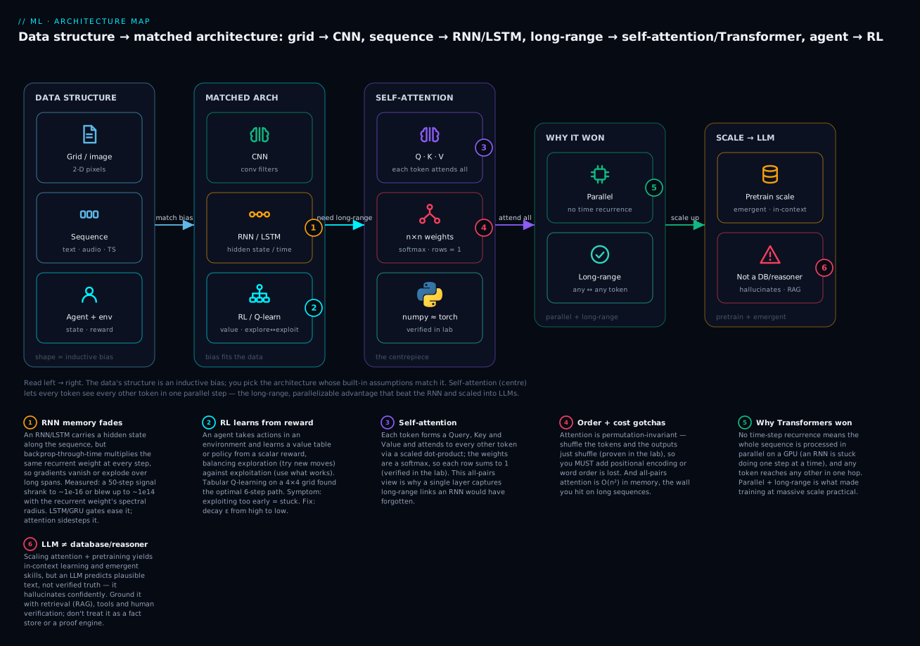
Everything from here fills in that picture: the sequence models (RNN, LSTM), the Transformer and its self-attention centrepiece, the generative families, and reinforcement learning. Where a piece is small enough to run, we run it.
Sequence models: why an MLP or CNN struggles with order
A sequence is ordered data of variable length where earlier elements inform later ones: the words of a sentence, the daily prices of a stock, the samples of an audio waveform, the amino acids of a protein. Two properties make sequences hostile to the MLP, and it is worth naming them precisely because the RNN and Transformer are engineered around exactly these two facts.
Variable length. A sentence can be 3 words or 300. An MLP has a fixed number of input neurons, so it cannot, in principle, accept “a sentence” — only “exactly N numbers.” You can hack around it (pad or truncate to a fixed length, or average the word vectors into one fixed vector — a “bag of words”), but padding wastes computation and averaging destroys the order entirely, which is the second problem.
Order carries meaning. “The dog bit the man” and “the man bit the dog” contain identical words in identical counts; only the order distinguishes a normal Tuesday from a news story. A bag-of-words model sees them as identical. An MLP fed the words in fixed slots sees position 1 and position 4 as unrelated inputs with independent weights — it has no built-in machinery that says “this is a sequence flowing left to right, and what came before conditions what comes now.” It can learn some of this given enough data and slots, but it is fighting its own architecture, which assumes no such structure.
A CNN handles local order well — a 1-D convolution over a sequence captures short patterns (“New York”, “not good”) the way a 2-D conv captures edges — and 1-D CNNs are genuinely used for text and time series. But a convolution’s receptive field is local by design: a filter of width 5 sees 5 neighbouring elements. To connect word 1 to word 100 you must stack many conv layers to grow the receptive field, and even then long-range dependencies are indirect. The CNN’s inductive bias (“nearby things relate”) is exactly wrong for “the pronoun in sentence 10 refers to the name in sentence 1.”
| Approach to sequences | Variable length? | Preserves order? | Long-range links? | Verdict |
|---|---|---|---|---|
| MLP, padded/truncated | forced to fixed N | weakly (position slots) | poorly | wastes compute, brittle |
| MLP, bag-of-words | yes (averaged) | no — order destroyed | no | loses the point of a sequence |
| 1-D CNN | yes (sliding) | locally | only via deep stacks | good for local patterns, weak long-range |
| RNN / LSTM | yes (any length) | yes (built-in) | limited (fading memory) | the classic sequence tool |
| Transformer | yes (up to a max) | via positional encoding | yes (all-pairs) | the modern default |
The RNN was the first architecture built specifically for the two properties above, so we build one next.
RNNs: a hidden state carried across time
The recurrent neural network’s idea is beautifully simple: process the sequence one element at a time, and carry a running summary — the hidden state — from each step to the next. At every time step the RNN combines the current input with the hidden state left over from the previous step, producing a new hidden state. That hidden state is the network’s memory: a fixed-size vector that, in principle, summarizes everything seen so far. The same weights are reused at every step, which is what lets a single small network process a sequence of any length — the answer to the variable-length problem.
Formally, for input x_t at step t and previous hidden state h_{t-1}:
$$h_t = \tanh(x_t W_{xh} + h_{t-1} W_{hh} + b_h)$$
W_xh maps the current input into hidden space; W_hh — the recurrent weight — maps the previous hidden state forward; tanh is the nonlinearity. Read it as: the new memory is a squashed blend of what I just saw and what I remembered. Let us build exactly this in numpy and watch the hidden state evolve as it consumes a short 4-step sequence.
import numpy as np

# A vanilla RNN cell processing a short sequence, hidden state carried across time.
# h_t = tanh(x_t @ W_xh + h_{t-1} @ W_hh + b_h)
rng = np.random.default_rng(0)

T, in_dim, hidden = 4, 2, 3                    # 4 time steps, 2 input features, 3 hidden units
W_xh = rng.normal(0, 0.5, (in_dim, hidden))    # input -> hidden
W_hh = rng.normal(0, 0.5, (hidden, hidden))    # hidden -> hidden (the recurrence)
b_h  = np.zeros(hidden)

xs = np.array([[1.0, 0.0],                      # a toy 4-step input sequence
               [0.5, 0.5],                      #   (imagine 4 words / 4 timesteps)
               [0.0, 1.0],
               [1.0, 1.0]])

h = np.zeros(hidden)                            # h_0: the initial memory is empty
print("h_0 (start):", h.round(4))
for t in range(T):
    h = np.tanh(xs[t] @ W_xh + h @ W_hh + b_h)  # SAME weights reused every step
    print(f"step {t+1}: x={xs[t]}  ->  h_{t+1} = {h.round(4)}")

print("\nfinal hidden state (summary of whole sequence):", h.round(4))
print("W_xh shape:", W_xh.shape, " W_hh shape:", W_hh.shape, " (reused at every step)")
h_0 (start): [0. 0. 0.]
step 1: x=[1. 0.]  ->  h_1 = [ 0.0628 -0.066   0.3097]
step 2: x=[0.5 0.5]  ->  h_2 = [-0.2162 -0.1494  0.0341]
step 3: x=[0. 1.]  ->  h_3 = [-0.0336 -0.3162  0.2284]
step 4: x=[1. 1.]  ->  h_4 = [ 0.0279 -0.2695  0.3487]
W_xh shape: (2, 3)  W_hh shape: (3, 3)  (reused at every step)
Watch the hidden state h change at every step — it starts empty (h_0 = [0, 0, 0]), and each new input rotates and reshapes it. Step 4’s hidden state [0.0279, -0.2695, 0.3487] depends, through the chain of W_hh multiplications, on all four inputs, not just the last — that is the memory. For a classification task (sentiment of a sentence) you would feed this final hidden state to an output layer; for a translation or generation task you would emit an output at every step. The crucial structural facts: the same W_xh and W_hh are reused at every step (so any length works), and information flows forward only through that one fixed-size h bottleneck.
Is this a real RNN, or did we just make up an equation? Cross-check it against PyTorch’s built-in nn.RNNCell, copying our exact weights into it (PyTorch computes W_ih @ x where we compute x @ W_xh, so we transpose):
import torch, torch.nn as nn
cell = nn.RNNCell(in_dim, hidden, bias=True).double()
with torch.no_grad():
    cell.weight_ih.copy_(torch.tensor(W_xh.T))     # torch uses W_ih @ x -> transpose ours
    cell.weight_hh.copy_(torch.tensor(W_hh.T))
    cell.bias_ih.zero_(); cell.bias_hh.zero_()
ht = torch.zeros(1, hidden, dtype=torch.double)
for t in range(T):
    ht = cell(torch.tensor(xs[t:t+1]), ht)
print("numpy final h:", h.round(4))
print("torch final h:", ht.detach().numpy().round(4).ravel())
print("match?", np.allclose(h, ht.detach().numpy().ravel(), atol=1e-6))
# => numpy final h: [ 0.0279 -0.2695  0.3487]
# => torch final h: [ 0.0279 -0.2695  0.3487]
# => match? True
They agree to machine precision. Our four lines of numpy are a vanilla RNN — the framework’s version is the same arithmetic with autograd and a GPU kernel attached (the convenience you met in PyTorch & Keras: Your First Models). Here is the anatomy in one table:
| Symbol | Meaning | Shape (our net) | Role |
|---|---|---|---|
x_t |
input at step t |
(2,) |
current element of the sequence |
h_t |
hidden state after step t |
(3,) |
the running memory / summary |
W_xh |
input→hidden weights | (2, 3) |
how the current input enters memory |
W_hh |
hidden→hidden (recurrent) weights | (3, 3) |
how the past propagates forward |
b_h |
hidden bias | (3,) |
baseline offset |
tanh |
activation | — | squashes memory into (−1, 1) |
RNNs come in a few standard shapes depending on how inputs and outputs line up, and the vocabulary is worth knowing because it names most sequence tasks:
| Shape | Inputs → outputs | Example task |
|---|---|---|
| one-to-many | one input → a sequence | image → caption |
| many-to-one | a sequence → one output | sentence → sentiment label |
| many-to-many (aligned) | sequence → sequence, same length | per-word part-of-speech tagging |
| many-to-many (seq2seq) | sequence → sequence, different length | translation (encoder + decoder) |
The vanilla RNN is elegant and it works on short sequences — but it has a crippling flaw on long ones, and that flaw is the reason LSTMs, and ultimately Transformers, exist.
The vanishing and exploding gradient problem
Training an RNN means backpropagating the error not just through layers but through time — unrolling the recurrence across every step and applying the chain rule from the last step back to the first. This is backpropagation through time (BPTT), and it has a structural pathology. To get the gradient at step 1 from an error at step 50, you multiply by the recurrent Jacobian (roughly W_hh times tanh') once per step you travel back — about 50 times. Repeated multiplication by the same matrix is a recipe for exponential behaviour: if that matrix tends to shrink vectors, the gradient vanishes toward zero; if it tends to grow them, the gradient explodes toward infinity. Either way, the early steps stop learning correctly, and the RNN cannot connect distant events.
You do not have to take this on faith — the exponential is easy to exhibit. The key quantity is the recurrent weight’s spectral radius (its largest eigenvalue magnitude): below 1, signals shrink; above 1, they grow. Push a unit gradient back through 50 steps for three different weight scales:
import numpy as np

def signal_decay(scale, T=50):
    rng = np.random.default_rng(0)
    W = rng.normal(0, scale, (4, 4))
    g = np.ones(4)                       # a unit gradient entering at the last step
    for _ in range(T):
        g = 0.9 * (W.T @ g)              # 0.9 stands in for a typical tanh' in the active region
    return np.linalg.norm(g)

for scale in (0.3, 0.6, 1.2):
    rng = np.random.default_rng(0)
    W = rng.normal(0, scale, (4, 4))
    radius = max(abs(np.linalg.eigvals(W)))
    print(f"W scale={scale}: spectral radius={radius:.3f}  ->  |grad| after 50 steps = {signal_decay(scale):.3e}")
W scale=0.3: spectral radius=0.536  ->  |grad| after 50 steps = 2.842e-16
W scale=0.6: spectral radius=1.072  ->  |grad| after 50 steps = 3.200e-01
W scale=1.2: spectral radius=2.145  ->  |grad| after 50 steps = 3.603e+14
Three regimes, three fates for the gradient reaching the first time step:
| Recurrent weight scale | Spectral radius | Gradient after 50 steps | What happens |
|---|---|---|---|
| small (0.3) | 0.536 (< 1) | 2.8×10⁻¹⁶ |
vanishes — early steps get ~zero signal, cannot learn long-range |
| medium (0.6) | 1.072 (≈ 1) | 3.2×10⁻¹ |
roughly stable — the narrow, hard-to-hit sweet spot |
| large (1.2) | 2.145 (> 1) | 3.6×10¹⁴ |
explodes — gradients overflow, weights go to nan |
The vanishing case (~10⁻¹⁶) means an error at word 50 sends essentially no corrective signal back to word 1 — so a vanilla RNN struggles to learn that a sentence’s subject (word 1) governs its verb (word 40). The exploding case (~10¹⁴) blows the weights up and nans the loss. The stable middle is a razor’s edge that ordinary training does not reliably sit on. Exploding gradients have a cheap patch — gradient clipping, capping the gradient’s norm — but vanishing gradients are structural and demanded a new cell design. That design is the LSTM.
LSTM and GRU: gates that let memory and gradients flow
The Long Short-Term Memory cell (LSTM, 1997) fixes vanishing gradients with one structural change: alongside the hidden state it maintains a separate cell state C_t — a memory conveyor belt that runs straight down the sequence with only minor, gated linear interactions. Because information can travel along the cell state with an addition rather than a repeated matrix multiply, the gradient can flow across many steps without vanishing. Small neural gates (each a sigmoid producing values in 0–1, acting as soft on/off valves) decide what to erase, what to write, and what to read at each step. This lesson does not build an LSTM from scratch — the gating arithmetic is fiddly and the point is conceptual — so treat the following as the map, not a runnable derivation.
| Gate | Question it answers | Mechanism |
|---|---|---|
| Forget gate | what to erase from memory? | sigmoid over [h_{t-1}, x_t], multiplies the old cell state |
| Input gate | what new info to write? | sigmoid decides how much; a tanh proposes what |
| Cell state update | the memory conveyor belt | C_t = forget·C_{t-1} + input·candidate (mostly addition!) |
| Output gate | what to read out as h_t? |
sigmoid gates a tanh of the cell state |
The crucial line is the cell-state update: C_t = f_t · C_{t-1} + i_t · \tilde{C}_t. When the forget gate f_t is near 1 and the input gate near 0, the cell state passes through unchanged — memory persists indefinitely, and the gradient with it, because the derivative of that path is just f_t (near 1) rather than a shrinking product of weights. That is the whole trick: an additive, gated highway for memory instead of a multiplicative bottleneck.
The Gated Recurrent Unit (GRU, 2014) is a streamlined LSTM: it merges the cell and hidden state and uses two gates (reset, update) instead of three. It has fewer parameters, trains a little faster, and performs comparably on most tasks — a reasonable default when you want recurrence with less machinery.
| Cell | States | Gates | Vs. vanilla RNN |
|---|---|---|---|
| Vanilla RNN | hidden h |
none | baseline; vanishing gradients kill long-range |
| LSTM | hidden h + cell C |
forget, input, output (3) | additive memory highway → learns long-range |
| GRU | hidden h only |
reset, update (2) | fewer params, ~same performance, faster |
For roughly two decades, LSTMs were the state of the art for sequences — machine translation, speech recognition, text generation all ran on them, and they remain a fine choice for modest-length time series today. Their honest use cases:
| Task | Why an LSTM fits | Modern reality |
|---|---|---|
| Time-series forecasting | modest-length, order-critical, limited data | still competitive vs. Transformers |
| Speech recognition | long audio sequences, streaming | largely moved to Transformers |
| Text generation / translation | order + memory | replaced by Transformers |
| Sensor / IoT streams | online, low-latency, small models | LSTM/GRU still practical |
But LSTMs inherit one flaw they cannot fix: they are inherently sequential. To compute step 50 you must first compute steps 1 through 49, in order — the recurrence forbids parallelism within a sequence. On modern hardware (GPUs, which are massively parallel) that is a catastrophe for training speed on long sequences and huge datasets. And their long-range memory, though vastly better than a vanilla RNN’s, still fades over hundreds of steps. In 2017 a new architecture removed the recurrence entirely, connected every position to every other directly, and processed the whole sequence in parallel. It won so decisively that it now underlies essentially all of modern NLP and much of vision. It is the Transformer.
Transformers: self-attention from scratch
The Transformer’s core idea is self-attention: instead of passing information step by step through a hidden state, let every element look directly at every other element in a single operation, and learn how much each should attend to each. “The animal didn’t cross the street because it was tired” — to resolve “it,” the model needs word “it” to attend to “animal,” seven words back, directly, not through a chain of fading hidden states. Self-attention makes that a one-hop connection, and it does so for all pairs at once, in parallel.
The mechanism gives every token three learned vectors, and the fruit-market analogy is the standard one: each token issues a Query (what am I looking for?), advertises a Key (what do I offer?), and holds a Value (the content I’ll pass on if attended to). A token’s output is a weighted average of all tokens’ Values, where the weights come from how well its Query matches each Key.
| Vector | Question it answers | How it’s made |
|---|---|---|
| Query (Q) | “what am I looking for?” | X @ W_q |
| Key (K) | “what do I contain / offer?” | X @ W_k |
| Value (V) | “what will I contribute if attended to?” | X @ W_v |
The full operation is scaled dot-product attention, four steps: (1) score every Query against every Key with a dot product; (2) scale by 1/√d_k to keep the scores from getting too large; (3) softmax each row into weights that sum to 1; (4) use those weights to average the Values.
$$\text{Attention}(Q,K,V) = \text{softmax}!\left(\frac{QK^\top}{\sqrt{d_k}}\right)V$$
Let us compute it by hand on three tokens (imagine the words “the,” “cat,” “sat”), each a 4-dimensional embedding, and print the attention-weight matrix so you can see the structure:
import numpy as np
rng = np.random.default_rng(42)
d_model = d_k = 4

X = np.array([[1.0, 0.0, 1.0, 0.0],           # 3 token embeddings: "the", "cat", "sat"
              [0.0, 2.0, 0.0, 1.0],
              [1.0, 1.0, 0.0, 0.0]])

W_q = rng.normal(0, 0.5, (d_model, d_k))
W_k = rng.normal(0, 0.5, (d_model, d_k))
W_v = rng.normal(0, 0.5, (d_model, d_k))

Q = X @ W_q          # (3,4)  what each token is "looking for"
K = X @ W_k          # (3,4)  what each token "offers"
V = X @ W_v          # (3,4)  the content each token passes on

def softmax(z):
    z = z - z.max(axis=-1, keepdims=True)     # subtract max for numerical stability
    e = np.exp(z)
    return e / e.sum(axis=-1, keepdims=True)

scores = Q @ K.T / np.sqrt(d_k)               # (3,3) scaled similarity
attn   = softmax(scores)                       # (3,3) each ROW is a probability distribution
out    = attn @ V                              # (3,4) weighted blend of all Values

np.set_printoptions(precision=4, suppress=True)
print("attention weight matrix (rows = queries, cols = keys):")
print(attn)
print("\neach row sums to 1?", attn.sum(axis=1).round(6))
print("\noutput (one context vector per token), shape", out.shape)
print(out)
attention weight matrix (rows = queries, cols = keys):
[[0.2836 0.3981 0.3183]
 [0.2823 0.4046 0.313 ]
 [0.3096 0.3546 0.3358]]

each row sums to 1? [1. 1. 1.]

output (one context vector per token), shape (3, 4)
[[-0.089  -0.5926 -0.195   0.7797]
 [-0.0879 -0.5928 -0.1969  0.7792]
 [-0.0891 -0.5788 -0.1805  0.7798]]
Read the attention matrix carefully, because it is the mechanism. Row 0 is token “the” acting as a Query: it attends 0.284 to “the” (itself), 0.398 to “cat,” and 0.318 to “sat.” Every row sums to exactly 1 — each token spreads a total attention budget of 1 across all tokens, which is what the softmax guarantees. Notice token 1 (“cat”) draws the most attention from every query (the middle column is largest in every row) — its Key happened to align with the Queries, so it dominates the blend. The output row for each token is that token’s Query-weighted average of the three Value vectors — its new, context-aware representation. This is not a metaphor for attention; it is attention, the same computation running inside every Transformer on earth.
Confirm it against PyTorch’s optimized kernel:
import torch, torch.nn.functional as F
Qt, Kt, Vt = torch.tensor(Q), torch.tensor(K), torch.tensor(V)
out_torch = F.scaled_dot_product_attention(Qt, Kt, Vt)
print("matches torch.nn.functional.scaled_dot_product_attention?",
      np.allclose(out, out_torch.numpy(), atol=1e-6))
# => matches torch.nn.functional.scaled_dot_product_attention? True
Our numpy attention equals PyTorch’s to machine precision. Two details in that code earn their place. The 1/√d_k scaling matters because dot products grow with dimension; without it, large scores push the softmax into a near-one-hot regime where gradients vanish. You can see the scaling gentle the scores:
raw scores QKᵀ:                scaled by 1/√4 = 0.5:
[[1.327 2.005 1.558]           [[0.663 1.003 0.779]
 [0.679 1.399 0.885]            [0.339 0.699 0.443]
 [1.151 1.423 1.314]]           [0.576 0.711 0.657]]
And the z - z.max() in the softmax is the numerical-stability trick from earlier lessons — it prevents exp from overflowing on large scores while leaving the result unchanged. Here is the operation as a table of shapes, the thing to keep straight when you build one:
| Step | Operation | Shape (3 tokens, d=4) | Meaning |
|---|---|---|---|
| Project | Q,K,V = X @ W_{q,k,v} |
(3,4) each |
three views of each token |
| Score | Q @ K.T |
(3,3) |
Query·Key similarity, all pairs |
| Scale | / √d_k |
(3,3) |
keep scores modest |
| Weight | softmax(row) |
(3,3), rows sum to 1 |
attention distribution per token |
| Blend | weights @ V |
(3,4) |
context vector per token |
Attention’s cost is written in that (3,3) score matrix: for n tokens it is n × n, so both compute and memory scale as O(n²). Fine for n=3; for a 100,000-token document it is 10 billion entries, and it is the central engineering wall of long-context Transformers (addressed by sparse, linear, and flash-attention variants). Remember that number — it reappears in the troubleshooting table.
Multi-head attention and positional encoding
Two refinements turn one attention operation into a Transformer layer, and both are essential rather than cosmetic.
Multi-head attention runs several attention operations in parallel — each with its own W_q, W_k, W_v — then concatenates their outputs. Why? One attention “head” learns one kind of relationship; with eight heads, the model can simultaneously track, say, syntactic agreement in one head, coreference (“it” → “animal”) in another, and positional adjacency in a third. Each head is lower-dimensional (the model dimension is split across heads, so it costs about the same as one full-width head), and the diversity is the point. It is the difference between reading a sentence once and reading it eight times looking for eight different things.
| Aspect | Single-head attention | Multi-head attention |
|---|---|---|
| Projections | one W_q,W_k,W_v set |
h independent sets (e.g. 8) |
| What it captures | one relationship type | many relationships at once |
| Dimension per head | full d_model |
d_model / h (split) |
| Output | one context vector | h vectors concatenated, then projected |
| Cost | O(n²·d) | ≈ O(n²·d) (same, parallelized) |
Positional encoding solves a subtle, fatal problem: self-attention has no notion of order. Look again at the attention formula — it is a sum over all tokens, and a sum does not care about order. Shuffle the input tokens and the outputs shuffle identically, but no token’s own representation changes. That means “dog bites man” and “man bites dog” would produce the same set of representations. For a mechanism meant to model language, that is a disaster, and it is easy to prove:
perm = [2, 0, 1]                              # shuffle the token order
def attention(X):
    Q, K, V = X @ W_q, X @ W_k, X @ W_v
    return softmax(Q @ K.T / np.sqrt(d_k)) @ V

out_perm = attention(X[perm])
print("attention(shuffled X) == shuffle of attention(X)?",
      np.allclose(out_perm, attention(X)[perm], atol=1e-6))
# => attention(shuffled X) == shuffle of attention(X)? True
True confirms the flaw: attention is permutation-invariant (more precisely, permutation-equivariant) — order carries no information whatsoever. The fix is to add a position-dependent signal to each token’s embedding before attention, so that “cat at position 1” and “cat at position 3” enter with different vectors. The original Transformer used fixed sinusoidal encodings — sines and cosines of the position at geometrically spaced frequencies:
def positional_encoding(seq_len, d_model):
    pos = np.arange(seq_len)[:, None]
    i = np.arange(d_model)[None, :]
    angle = pos / (10000 ** (2 * (i // 2) / d_model))
    return np.where(i % 2 == 0, np.sin(angle), np.cos(angle))

PE = positional_encoding(4, 4)
print("positional encodings for positions 0..3 (dim=4):")
print(PE.round(4))

def attend_with_pe(X):                         # stamp position onto each SLOT, then attend
    return attention(X + PE[:len(X)])

print("\nafter adding PE, still permutation-invariant?",
      np.allclose(attend_with_pe(X[perm]), attend_with_pe(X)[perm], atol=1e-6))
positional encodings for positions 0..3 (dim=4):
[[ 0.      1.      0.      1.    ]
 [ 0.8415  0.5403  0.01    1.    ]
 [ 0.9093 -0.4161  0.02    0.9998]
 [ 0.1411 -0.99    0.03    0.9996]]

after adding PE, still permutation-invariant? False
The flip from True to False is the whole lesson of positional encoding: once each position carries a distinct signature, shuffling the tokens genuinely changes the result — order now matters. Miss this step and your Transformer is a sophisticated bag-of-words. Modern models often use learned or rotary (RoPE) position encodings instead of sinusoids, but the necessity is identical.
| Position scheme | How it works | Used by |
|---|---|---|
| Sinusoidal (fixed) | sin/cos at geometric frequencies, added to embeddings | original Transformer |
| Learned absolute | a trainable vector per position | BERT, GPT-2 |
| Rotary (RoPE) | rotate Q/K by position-dependent angles | LLaMA, most recent LLMs |
| ALiBi | bias attention scores by distance | some long-context models |
Encoder, decoder, and why Transformers won
A full Transformer stacks these attention layers into blocks, each block wrapping multi-head attention and a small position-wise MLP with two engineering staples that make deep stacks trainable — residual connections (add the input back to the output, giving gradients a clean path, the same vanishing-gradient remedy from the deep-net lesson) and layer normalization (stabilize activations). Blocks come in two flavours:
| Block type | Attention pattern | Sees | Job | Example models |
|---|---|---|---|---|
| Encoder | bidirectional self-attention | the whole input at once | build rich representations | BERT (classification, embeddings) |
| Decoder | masked (causal) self-attention | only tokens so far | generate the next token | GPT family (text generation) |
| Encoder–decoder | encoder + cross-attention | input + generated output | transform one sequence to another | T5, translation |
The decoder’s causal mask is what makes generation honest: when predicting word t, the mask zeroes out attention to words t+1 onward, so the model cannot “cheat” by peeking at the future it is supposed to predict. GPT-style models are decoder-only stacks; the whole of “generate the next token, append it, repeat” is masked self-attention run autoregressively.
Now the payoff — why the Transformer displaced the LSTM so completely. Two reasons, both consequences of removing recurrence:
| Property | RNN / LSTM | Transformer |
|---|---|---|
| Parallelism within a sequence | none — step t needs step t−1 |
full — all positions at once |
| Path length between distant tokens | O(n) (through the hidden chain) | O(1) (direct attention) |
| Training speed on long sequences | slow (sequential) | fast (GPU-parallel) |
| Long-range dependency modelling | fades with distance | direct, all-pairs |
| Memory / compute cost | O(n) | O(n²) (the tradeoff) |
| Positional information | implicit in order of processing | must be injected (positional encoding) |
The first row is the one that changed history. An LSTM’s recurrence forbids parallelism — you cannot compute step 50 before step 49 — which wastes the massively parallel GPUs that modern training runs on. The Transformer computes all positions simultaneously (one big matrix multiply), so it saturates the hardware and trains dramatically faster, which means you can afford to train it on far more data and far more parameters. The second row — any token reaches any other in one attention hop instead of a fading chain — means long-range dependencies are modelled directly. Parallel training plus direct long-range modelling is the combination that made it practical to scale to billions of parameters and trillions of tokens. That scale is what produced large language models, and it is worth being precise and honest about what scale did and did not buy. (For the applied NLP side — tokenization, embeddings, fine-tuning a Transformer for classification — see NLP: Text Classification, Sentiment & Transformers.)
Scaling to LLMs: what pretraining actually buys
A large language model is a decoder-only Transformer with billions of parameters, trained on a large fraction of the public internet with one deceptively simple objective: predict the next token. That is the entire pretraining task — given a prefix, guess the next word-piece, and adjust weights when wrong, over trillions of tokens. Everything an LLM appears to “know” is a side effect of getting very, very good at that one prediction. Being honest about this is the difference between using LLMs well and being fooled by them.
| Concept | What it means | Honest caveat |
|---|---|---|
| Pretraining | next-token prediction over a huge corpus | learns language patterns + world co-occurrences, not verified facts |
| Emergent behaviour | capabilities (arithmetic, translation) appearing only past a scale threshold | real but unpredictable; not “understanding” |
| In-context learning | learning a task from examples in the prompt, no weight updates | pattern-matching on the prompt, bounded by context window |
| Fine-tuning | further training on task/domain data | adapts style/format; can still hallucinate |
| RLHF | reinforcement learning from human feedback to align outputs | makes it helpful/harmless, not truthful |
| RAG | retrieval-augmented generation: fetch documents, put them in the prompt | grounds answers in real sources — the fix for hallucination |
| Prompting | crafting the input to steer the output | cheapest lever; brittle, model-specific |
The two ideas that most surprise newcomers are in-context learning (show the model three examples of a task in the prompt and it does the fourth — with no gradient updates, just pattern completion) and emergent behaviour (some capabilities simply do not exist at small scale and appear, often abruptly, past some parameter/data threshold). Both are genuine and both are routinely over-read. An LLM is a spectacularly capable text predictor; it is not a database (it stores patterns, not verified records, and will fabricate a plausible citation as readily as a real one) and not a reasoner (it predicts what a reasoning trace looks like, which usually but not always coincides with correct reasoning). The engineering discipline that follows: for factual accuracy, ground it with retrieval (RAG) and tools; for reliability, verify its outputs; never treat a confident answer as a checked one. This honesty is not pessimism — it is the operating manual. The deployment side (serving models, latency, cost) is its own subject, covered in the MLOps material of this course.
Generative and other families, briefly and honestly
Not every architecture classifies or predicts; a whole branch of deep learning generates — learns the distribution of the data well enough to produce new samples. Four families matter, and one honest paragraph each is the right dose at this altitude.
Autoencoders learn to compress data to a small “bottleneck” code and reconstruct it, training on the reconstruction error alone (no labels — this is self-supervised). The encoder half is a learned, nonlinear dimensionality reducer (a more powerful cousin of PCA); the uses are compression, denoising, and anomaly detection (things that reconstruct badly are anomalies). A plain autoencoder is not really a generator — its latent space has holes — which is what the VAE fixes.
Variational autoencoders (VAEs) make the bottleneck a probability distribution rather than a point, so the latent space is smooth and continuous and you can sample new data from it. They generate coherent but characteristically blurry images — the probabilistic objective averages over possibilities. VAEs are prized when you want a well-behaved latent space to interpolate or manipulate, less so when you want crisp photorealism.
Generative adversarial networks (GANs) pit two networks against each other: a generator invents fake samples and a discriminator tries to tell fakes from real, each improving the other in a minimax game. GANs produced the first strikingly photorealistic faces (the “this person does not exist” era) and remain strong for sharp image synthesis, but they are notoriously unstable to train — mode collapse (the generator produces one thing), non-convergence, and delicate balance between the two networks are standard headaches.
Diffusion models learn to reverse a gradual noising process: take an image, add noise over many steps until it is pure static, then train a network to undo it one step at a time; to generate, start from pure noise and denoise into a sample. They now dominate high-quality image and audio generation (Stable Diffusion, DALL·E, Midjourney) because they train stably (unlike GANs) and produce sharp, diverse output (unlike VAEs). The cost is slow sampling — many denoising steps per image — though that gap is closing.
| Family | Learns by | Generates | Strength | Honest weakness |
|---|---|---|---|---|
| Autoencoder | reconstruction error | (not really — compresses) | denoising, anomaly detection | latent space has gaps |
| VAE | reconstruction + distribution match | new samples from a smooth latent | controllable latent space | blurry output |
| GAN | generator vs. discriminator game | sharp, realistic samples | photorealism | unstable training, mode collapse |
| Diffusion | reverse a noising process | high-quality images/audio | stable training + sharp + diverse | slow sampling (many steps) |
Reinforcement learning basics
Everything so far is supervised or self-supervised — you have a dataset and a target (a label, the next token, the input itself) and you minimize a loss against it. Reinforcement learning (RL) is a fundamentally different paradigm: there is no dataset of correct answers. An agent acts in an environment, and all it receives is a scalar reward — a number saying “that was good” or “that was bad,” often delayed and sparse. The agent must discover, by trial and error, a strategy that maximizes cumulative reward. This is how you train a game player, a robot, or the alignment step (RLHF) of an LLM — anywhere the right action is not labelled but evaluated.
The loop and its vocabulary are the foundation; learn these seven words and you can read any RL paper’s setup:
| Term | Meaning | Gridworld example |
|---|---|---|
| Agent | the learner/decider | the thing moving on the grid |
| Environment | the world it acts in | the 4×4 grid |
| State (s) | the current situation | which cell the agent is in |
| Action (a) | a choice available | up / right / down / left |
| Reward ® | scalar feedback after an action | +1 for reaching the goal, else 0 |
| Policy (π) | the agent’s strategy: state → action | “in cell 6, go right” |
| Value (Q or V) | expected future reward | how good is this state/action long-term |
At each step the agent observes the state, picks an action via its policy, and the environment returns a reward and the next state; the agent updates its policy to do better. The central difficulty, which has no equivalent in supervised learning, is the exploration–exploitation tradeoff: should the agent exploit the best action it currently knows, or explore an untried action that might be better? Always exploiting gets stuck in a rut (it never discovers the shortcut); always exploring never cashes in what it learned. The standard cheap balance is ε-greedy: with probability ε take a random action (explore), otherwise take the best known action (exploit) — and typically decay ε from high to low, so the agent explores boldly early and exploits its knowledge later.
Q-learning and the Bellman update
Q-learning is the classic value-based algorithm. It learns a table Q[state, action] estimating the total future (discounted) reward of taking that action in that state and behaving well thereafter. The learning rule is the Bellman update — after taking action a in state s, seeing reward r, and landing in s':
$$Q(s,a) \leftarrow Q(s,a) + \alpha\big[,r + \gamma\max_{a’}Q(s’,a’) - Q(s,a),\big]$$
In words: nudge Q(s,a) toward the reward you just got plus the discounted value of the best next move. The bracket is the temporal-difference error — the gap between your old estimate and a better one built from real experience. α is the learning rate; γ (the discount factor, 0–1) trades immediate versus future reward — below 1, it makes the agent prefer reaching the goal sooner (each step of delay shaves value), which is exactly what makes it find short paths.
Let us watch it learn. A 4×4 gridworld, start at the top-left (state 0), goal at the bottom-right (state 15), reward +1 only at the goal. The agent knows nothing at the start — the Q-table is all zeros — and must learn purely from the reward signal:
import numpy as np
rng = np.random.default_rng(0)

N, GOAL = 4, 15
ACTIONS = {0: (-1, 0), 1: (0, 1), 2: (1, 0), 3: (0, -1)}   # up, right, down, left
ARROWS  = {0: "^", 1: ">", 2: "v", 3: "<"}

def step(s, a):
    r, c = divmod(s, N)
    dr, dc = ACTIONS[a]
    nr, nc = min(max(r + dr, 0), N - 1), min(max(c + dc, 0), N - 1)   # walls clamp
    ns = nr * N + nc
    return ns, (1.0 if ns == GOAL else 0.0), ns == GOAL

def greedy_policy(Q):
    return "\n".join(" ".join("G" if r*N+c == GOAL else ARROWS[int(np.argmax(Q[r*N+c]))]
                              for c in range(N)) for r in range(N))

def greedy_path_len(Q, cap=50):
    s, n = 0, 0
    while s != GOAL and n < cap:
        s, _, _ = step(s, int(np.argmax(Q[s]))); n += 1
    return n

alpha, gamma = 0.5, 0.95
Q = np.zeros((N * N, 4))
print("greedy policy BEFORE training (all-zero Q -> argmax picks 'up'):")
print(greedy_policy(Q))

for ep in range(500):
    eps = max(0.05, 1.0 - ep / 200)            # decay exploration 1.0 -> 0.05
    s = 0
    for _ in range(100):
        a = int(rng.integers(4)) if rng.random() < eps else int(np.argmax(Q[s]))
        ns, r, done = step(s, a)
        Q[s, a] += alpha * (r + gamma * Q[ns].max() - Q[s, a])       # Bellman update
        s = ns
        if done:
            break

print("\ngreedy policy AFTER 500 episodes:")
print(greedy_policy(Q))
print("\nQ-values at start state 0 (up,right,down,left):", Q[0].round(3))
print("optimal Q at start should be gamma^5 =", round(gamma ** 5, 4))
greedy policy BEFORE training (all-zero Q -> argmax picks 'up'):
^ ^ ^ ^
^ ^ ^ ^
^ ^ ^ ^
^ ^ ^ G

greedy policy AFTER 500 episodes:
> > v v
> > v v
> > > v
> > > G

Q-values at start state 0 (up,right,down,left): [0.735 0.774 0.774 0.735]
optimal Q at start should be gamma^5 = 0.7738
The learning is visible in the arrows. Before training, the all-zero Q-table’s argmax ties to action 0 (“up”) everywhere — a useless policy that would march the agent into the top wall forever. After 500 episodes, every cell’s arrow points toward the goal: the top rows say “go right,” the right column says “go down,” and following any arrow walks you to the bottom-right by the shortest route. Two numbers confirm the agent learned the optimal solution, not just a solution:
Adding one line inside the training loop — if ep+1 in (1,10,50,500): print(ep+1, greedy_path_len(Q)) — records how many steps the greedy policy takes from start to goal at each checkpoint (capped at 50 = “never arrives”):
after   1 episodes: never (>50) steps   (policy still useless)
after  10 episodes: 6 steps  <- optimal (3 rights + 3 downs)
after  50 episodes: 6 steps  <- optimal
after 500 episodes: 6 steps  <- optimal
The greedy path from start to goal drops from “never arrives” (before it has ever reached the goal) to exactly 6 steps — the true optimum for opposite corners of a 4×4 grid (3 rights + 3 downs). And the Q-value at the start for the best action is 0.774, matching the theoretical optimum γ⁵ = 0.95⁵ = 0.7738 almost exactly — because the +1 reward arrives 6 steps away and is discounted by γ once per step. The agent didn’t just stumble to the goal; it learned the discounted value of every move.
| State | Q-values (up, right, down, left) | Best action | Interpretation |
|---|---|---|---|
| 0 (start, top-left) | [0.735, 0.774, 0.774, 0.735] |
right or down (tie) | 6 steps from goal → γ⁵ ≈ 0.774 |
| 14 (left of goal) | [0.902, 1.000, 0.950, 0.901] |
right | 1 step from goal → reward 1.0 undiscounted |
One thing this run also teaches, by way of its own history: the exploration schedule was not incidental. An earlier attempt with a fixed low ε (0.1) never learned at all — the all-zero policy’s “up” bias sank the agent into the top-left corner, and 10% random moves were too few to ever stumble onto the distant goal, so the Q-table stayed all zeros. Decaying ε from 1.0 (pure exploration early, when the agent knows nothing) down to 0.05 fixed it. That is the exploration–exploitation tradeoff biting in practice, not in theory.
| ε (exploration) strategy | Behaviour | Outcome here |
|---|---|---|
| Fixed low (ε = 0.1) from the start | exploits a useless initial policy; barely explores | never reaches goal — Q stays all zeros |
| Fixed high (ε = 0.5) | explores well, but keeps acting randomly even when it knows better | learns, but noisy/slow |
| Decaying (1.0 → 0.05) | explores boldly early, exploits its knowledge late | learns the optimal path by episode ~10 |
Beyond tables: policy gradients and deep RL
Tabular Q-learning works only when states and actions are few enough to enumerate — a 4×4 grid has 16 states. A game of Go has more states than atoms in the universe; you cannot make a table. The fix is to approximate the value or policy with a neural network, which is where deep RL lives. This lesson does not train a deep-RL agent — they are famously sample-hungry and unstable, and an honest training run does not fit in a lesson — so the following is the conceptual map, explicitly not executed here.
| Method | Learns | Idea | Known for |
|---|---|---|---|
| Q-learning (tabular) | a value table | Bellman update on Q[s,a] |
small discrete problems (what we ran) |
| DQN (Deep Q-Network) | a value network | neural net approximates Q(s,a); replay buffer + target net for stability |
Atari from pixels (DeepMind, 2013–15) |
| Policy gradient (REINFORCE) | a policy directly | nudge action probabilities up when returns are high | continuous actions, stochastic policies |
| Actor–critic / PPO | policy (actor) + value (critic) | critic reduces the variance of the policy gradient | the modern default; robotics, RLHF |
Value-based methods (Q-learning, DQN) learn how good each action is and act greedily; policy-based methods (REINFORCE, PPO) learn the policy directly as a probability distribution over actions, which handles continuous action spaces (a robot joint angle) that a value table cannot. PPO (Proximal Policy Optimization), an actor–critic method that limits how far the policy moves per update for stability, is the workhorse behind most modern deep RL, including the RLHF that aligns LLMs.
Where RL genuinely shines, and where it genuinely hurts, in one honest ledger each:
| RL wins where… | Because |
|---|---|
| Games (Go, chess, Atari, StarCraft) | clear reward (win/score), cheap simulation, self-play generates data |
| Robotics / control | actions are sequential, no labelled “correct” trajectory exists |
| Recommendation / sequential decisions | optimizing long-term engagement, not one click |
| RLHF for LLMs | “good response” is evaluated by humans, not labelled — exactly RL’s shape |
| RL is brutally hard because… | Symptom |
|---|---|
| Sample-inefficient | needs millions–billions of interactions; only feasible with fast simulators |
| Unstable / high-variance | small changes → wildly different outcomes; runs don’t reproduce |
| Reward design is treacherous | agents exploit misspecified rewards literally (“reward hacking”) |
| Sparse/delayed rewards | if reward comes only at the end, credit assignment is very hard |
RL is not a drop-in replacement for supervised learning; it is the tool for problems shaped like sequential decisions evaluated by a reward, and it demands far more engineering care. Do not reach for it when a labelled dataset exists — supervised learning is vastly easier and more stable.
Which architecture for which problem
This is the master table — the practical distillation of the whole lesson. Start from the shape of your data and task, not from the architecture you find exciting.
| Data / problem | Reach for | Why (the inductive bias) | Not this |
|---|---|---|---|
| Tabular rows × columns | gradient-boosted trees (XGBoost) first, then MLP | no spatial/sequential structure to exploit | CNN/RNN/Transformer overkill |
| Images, video (grids) | CNN (or vision Transformer at scale) | locality + translation invariance | MLP (throws away spatial structure) |
| Short/local sequence patterns | 1-D CNN | local motifs, fast | RNN if patterns are local only |
| Sequences, modest length, limited data | LSTM / GRU | order + memory, data-efficient | Transformer (data-hungry) |
| Text / language, at scale | Transformer / LLM | long-range, parallel, pretrainable | RNN (slow, forgets) |
| Long-range dependencies (any modality) | Transformer (attention) | all-pairs, O(1) path length | RNN (fades over distance) |
| Generate images / audio | diffusion (or GAN) | stable, sharp, diverse samples | VAE if you need crisp output |
| Compress / denoise / find anomalies | autoencoder / VAE | learned reconstruction | GAN (no reconstruction) |
| Sequential decisions from a reward | reinforcement learning | no labels, learn from reward | supervised (no labels exist) |
| Small data, need interpretability | classical ML (linear, trees) | deep nets overfit + opaque | any deep architecture |
The meta-rule, the same one from ML fundamentals: match the architecture’s inductive bias to your data’s structure, start with the simplest thing that could work, and escalate only when the data’s structure demands it. A Transformer is not “better than” an LSTM in the abstract — it is better when you have long-range dependencies, lots of data, and parallel hardware, and worse when you have a few thousand rows where its hunger for data makes it overfit. Architecture selection is not fashion; it is fit.
Hands-on lab
Reproduce the three headline results end to end. Everything is seeded, so your numbers will match. One venv, three short files.
Setup (once):
python3 -m venv .venv && source .venv/bin/activate      # Windows: .venv\Scripts\activate
pip install numpy
pip install torch --index-url https://download.pytorch.org/whl/cpu
Step 1 — an RNN forward pass, hidden state evolving. Put this in lab_rnn.py.
import numpy as np
rng = np.random.default_rng(0)
T, in_dim, hidden = 4, 2, 3
W_xh = rng.normal(0, 0.5, (in_dim, hidden))
W_hh = rng.normal(0, 0.5, (hidden, hidden))
xs = np.array([[1.,0.], [0.5,0.5], [0.,1.], [1.,1.]])

h = np.zeros(hidden)
for t in range(T):
    h = np.tanh(xs[t] @ W_xh + h @ W_hh)        # same weights reused every step
    print(f"step {t+1}: h = {h.round(4)}")
# => step 1: h = [ 0.0628 -0.066   0.3097]
# => step 2: h = [-0.2162 -0.1494  0.0341]
# => step 3: h = [-0.0336 -0.3162  0.2284]
# => step 4: h = [ 0.0279 -0.2695  0.3487]
What just happened: the hidden state started empty and carried a running summary forward; step 4’s memory depends on all four inputs through the recurrent weight. That is the entire idea of an RNN.
Step 2 — self-attention, weights that sum to 1. Put this in lab_attention.py.
import numpy as np
rng = np.random.default_rng(42)
d = 4
X = np.array([[1.,0,1,0], [0,2.,0,1], [1.,1,0,0]])          # 3 tokens
W_q, W_k, W_v = (rng.normal(0, .5, (d, d)) for _ in range(3))
Q, K, V = X @ W_q, X @ W_k, X @ W_v

def softmax(z):
    z = z - z.max(-1, keepdims=True); e = np.exp(z); return e / e.sum(-1, keepdims=True)

attn = softmax(Q @ K.T / np.sqrt(d))            # (3,3) attention weights
print("attention weights:\n", attn.round(4))
print("row sums:", attn.sum(1).round(6))        # => [1. 1. 1.]
out = attn @ V
print("output shape:", out.shape)               # => (3, 4)

import torch, torch.nn.functional as F
ok = np.allclose(out, F.scaled_dot_product_attention(
    torch.tensor(Q), torch.tensor(K), torch.tensor(V)).numpy(), atol=1e-6)
print("matches torch?", ok)                      # => matches torch? True
What just happened: each token attended to all three tokens; every row of the weight matrix summed to 1 (a softmax), and your numpy result matched PyTorch’s optimized kernel exactly. You computed the core of a Transformer by hand.
Step 3 — Q-learning learns the optimal path. Put this in lab_qlearn.py (the full script is in the RL section above). Run it and read the arrows:
BEFORE:            AFTER 500 episodes:
^ ^ ^ ^            > > v v
^ ^ ^ ^            > > v v
^ ^ ^ ^            > > > v
^ ^ ^ G            > > > G
Q[start] = [0.735 0.774 0.774 0.735]   (optimal γ⁵ = 0.7738)
What just happened: from an all-zero table and only a +1-at-the-goal reward, the agent learned a policy whose every arrow leads to the goal by the shortest 6-step route, and the start-state value matched the discounted-reward optimum. No labels — just reward and the Bellman update.
Step 4 — break the exploration (see why ε matters). Change the ε line in lab_qlearn.py to a fixed low value and rerun:
eps = 0.1                                # fixed, low — instead of the decaying schedule
# => greedy policy stays "all up"; Q-table stays ~all zeros; agent never reaches the goal
What just happened: with too little early exploration, the agent exploited its useless initial policy and never discovered the goal — the exploration–exploitation tradeoff, failing in front of you. Restore the decay to fix it.
Common mistakes and troubleshooting
| Symptom / traceback | Cause | Fix |
|---|---|---|
| RNN loss stalls; can’t link distant events | vanishing gradients over long sequences | use LSTM/GRU, or switch to a Transformer |
RNN loss → inf/nan on long sequences |
exploding gradients | gradient clipping (cap the norm); smaller LR; better init |
| Transformer treats “dog bites man” = “man bites dog” | forgot positional encoding — attention is permutation-invariant | add positional encodings before the first attention layer |
CUDA out of memory / RAM blows up on long input |
attention is O(n²) in sequence length | shorter context; sparse/flash attention; chunk the input |
RuntimeError: mat1 and mat2 shapes cannot be multiplied |
wrong Q/K/V or weight shapes | print every .shape; W is (d_model, d_k); scores are (n, n) |
| Slow training, GPU underused, long sequences | used an RNN where a Transformer fits | Transformer parallelizes; RNN is sequential by construction |
| LLM invents a fake citation / wrong fact confidently | treating an LLM as a database/reasoner | ground with RAG + tools; verify outputs; never trust unchecked |
| Q-learning never improves; Q stays ~0 | agent never reaches reward — too little exploration | raise ε or decay it from high; check the reward is reachable |
| Q-learning oscillates / diverges | learning rate α too high; or γ ≥ 1 |
lower α; keep 0 < γ < 1 |
| RL agent finds a degenerate “cheat” | reward misspecified (reward hacking) | redesign the reward; penalize the exploit; add shaping carefully |
| RL learns nothing on a hard task | sparse/delayed reward, poor credit assignment | reward shaping; curriculum; a simpler sub-task first |
| Deep-RL run won’t reproduce; wildly different each seed | RL is high-variance / unstable | average over seeds; use PPO; tune carefully; expect fragility |
| Expecting RL to work like supervised learning | wrong mental model — no labelled dataset | if labels exist, use supervised learning instead |
nn.Transformer output ignores order |
didn’t add positional encoding / used wrong mask | add PE; use a causal mask for generation |
| Deep net on 2,000 tabular rows loses to XGBoost | wrong architecture for the data structure | match bias to data — tabular → boosting first |
Three failures cost the most time, in prose:
Forgetting positional encoding is the classic Transformer bug, and it is silent. The model trains, the loss falls, nothing errors — but the network is a bag-of-words that cannot tell “dog bites man” from “man bites dog,” because self-attention is permutation-invariant (we proved it: shuffle the tokens and the outputs just shuffle). There is no traceback; the only symptom is that order-dependent tasks plateau at mediocre accuracy. The discipline: whenever you assemble attention layers yourself, inject position first and verify — feed a sequence and its reverse and confirm the outputs differ. Frameworks’ high-level Transformer modules still expect you to add the encoding; it is not automatic.
Q-learning that never improves is almost always an exploration problem, not a learning-rate problem. Beginners tune α and γ for hours when the real issue is that the agent, acting greedily on a useless initial policy, never reaches the reward at all — so there is nothing to learn from, and the Q-table stays zero (we hit exactly this: fixed low ε left the agent sunk in the corner, never touching the goal). The fix is exploration: start ε high (even 1.0, fully random) so the agent stumbles onto the reward, then decay it. The diagnostic question is always “has the agent ever received the reward?” — if not, no amount of learning-rate tuning helps.
Reaching for the wrong architecture wastes weeks, and the tell is a mismatch between bias and data. An RNN on a long-sequence task with abundant data and GPUs is leaving enormous training speed on the table (it can’t parallelize) — use a Transformer. A Transformer on a few thousand tabular rows will overfit and lose to gradient boosting — use trees. A deep net on 500 examples will memorize them — use a linear model. The single most valuable habit is to name your data’s structure first (grid? sequence? long-range? agent-in-environment? flat table?) and let that pick the family, rather than picking a fashionable architecture and forcing your data into it.
Cheat-sheet
| Concept | Key formula / code | Note |
|---|---|---|
| RNN cell | h_t = tanh(x_t @ W_xh + h_{t-1} @ W_hh + b) |
same weights reused every step |
| RNN failure | vanishing/exploding gradient over time | fix: LSTM/GRU or Transformer |
| LSTM memory | C_t = f·C_{t-1} + i·C̃ (gated, additive) |
additive highway → long-range memory |
| GRU | LSTM with 2 gates, no separate cell state | fewer params, ~same performance |
| Self-attention | softmax(Q @ K.T / √d_k) @ V |
each token attends to all; rows sum to 1 |
| Q, K, V | X @ W_q, X @ W_k, X @ W_v |
query / key / value projections |
| Scaling | divide scores by √d_k |
keeps softmax gradients healthy |
| Multi-head | h parallel attentions, concatenated |
captures many relations at once |
| Positional encoding | add PE[pos] to embeddings |
mandatory — attention ignores order |
| Attention cost | O(n²) in sequence length | the long-context wall |
| Encoder / decoder | bidirectional / masked (causal) attention | BERT / GPT |
| Transformer win | parallel + O(1) path length | why it beat the RNN |
| LLM | decoder-only Transformer, next-token pretraining | not a database, not a reasoner |
| RAG | retrieve docs → put in prompt | the fix for hallucination |
| RL loop | state → action → reward → next state | learn from reward, no labels |
| Bellman update | Q[s,a] += α(r + γ·max Q[s'] − Q[s,a]) |
temporal-difference learning |
| ε-greedy | random w.p. ε, else best action | explore vs. exploit; decay ε |
Discount γ |
0–1, weights future reward | <1 → prefers shorter paths |
| Value vs policy RL | learn Q and act greedy / learn π directly |
DQN vs. PPO |
| Architecture rule | match inductive bias to data structure | grid→CNN, seq→RNN, long-range→Transformer, agent→RL |
Interview and exam questions
Q: What does it mean to say “an architecture is an inductive bias matched to the data”? Give three examples. A: An inductive bias is a built-in assumption about the data’s structure that lets a model learn efficiently from the right shape of input. A CNN assumes locality and translation invariance (good for images: nearby pixels relate, a cat is a cat anywhere). An RNN assumes order matters and the past informs the present (good for sequences). A Transformer assumes any element may depend on any other regardless of distance (good for long-range dependencies). Matching the bias to the data is why you pick a CNN for images and an RNN/Transformer for text rather than a plain MLP for both.
Q: Why does a plain MLP struggle with images and with sequences? A: With images, the MLP has no notion of spatial locality — flattening a grid throws away the fact that neighbouring pixels are related, forcing it to relearn every spatial relationship with a separate weight per pixel-neuron pair (millions of parameters). With sequences, it has a fixed input width (can’t take variable-length input) and treats input positions as unrelated slots (no built-in sense of order or flow). CNNs fix the first via shared local filters; RNNs and Transformers fix the second.
Q: Explain the vanishing/exploding gradient problem in RNNs. Why does it happen and how is it addressed?
A: Training an RNN backpropagates through time, multiplying by the recurrent Jacobian once per time step you travel back. Repeated multiplication by the same matrix is exponential: if its spectral radius is below 1, gradients vanish toward zero (early steps stop learning — can’t capture long-range dependencies); above 1, they explode toward inf/nan. Exploding gradients are patched with gradient clipping; vanishing gradients are structural and led to the LSTM/GRU, whose gated additive cell state lets memory and gradients flow across many steps without shrinking. Transformers avoid the problem entirely by removing recurrence.
Q: How does an LSTM solve what a vanilla RNN cannot?
A: An LSTM adds a separate cell state — a memory conveyor belt updated as C_t = forget·C_{t-1} + input·candidate, mostly by addition — plus sigmoid gates (forget, input, output) that decide what to erase, write, and read. Because memory travels along the cell state additively (derivative ≈ the forget gate, near 1) rather than through a repeated matrix multiply, the gradient does not vanish, so an LSTM learns long-range dependencies a vanilla RNN forgets. A GRU is a streamlined version with two gates and no separate cell state.
Q: Walk through scaled dot-product self-attention. Why does each row of the attention matrix sum to 1, and why divide by √d_k?
A: Each token is projected to a Query, Key, and Value. Scores are all-pairs dot products Q @ K.T (how well each Query matches each Key), scaled by 1/√d_k, then softmaxed row-wise into weights, which multiply the Values to produce each token’s context vector. Each row sums to 1 because it is a softmax — each token distributes a total attention budget of 1 across all tokens. The √d_k scaling counteracts dot products growing with dimension; without it, large scores push the softmax toward one-hot, where gradients vanish and training stalls.
Q: Why is positional encoding necessary in a Transformer? What breaks without it? A: Self-attention is a sum over all tokens, which is permutation-invariant — shuffle the input and the outputs just shuffle, so no token’s representation encodes where it sits. Without positional encoding the model is a bag-of-words: “dog bites man” and “man bites dog” produce identical representations. You add a position-dependent signal (sinusoidal, learned, or rotary) to each embedding before attention so identical tokens at different positions enter differently. It fails silently — no error, just poor accuracy on order-dependent tasks.
Q: Why did Transformers largely replace RNNs/LSTMs?
A: Two consequences of removing recurrence. First, parallelism: an RNN must compute step t after step t−1, so it can’t use parallel hardware within a sequence; a Transformer computes all positions at once (one matrix multiply), training far faster and thus scaling to far more data and parameters. Second, path length: any two tokens are connected directly by attention (O(1)) instead of through a fading O(n) hidden-state chain, so long-range dependencies are modelled directly. The cost is O(n²) attention memory. Parallel + direct long-range is what enabled LLM-scale training.
Q: In one honest paragraph, what is an LLM — and what is it not? A: A large language model is a decoder-only Transformer with billions of parameters, pretrained to predict the next token over a huge corpus. That single objective yields fluent language, in-context learning (doing a task from prompt examples with no weight updates), and emergent capabilities past certain scales. It is not a database (it stores statistical patterns, not verified records, and will fabricate plausible-looking facts and citations) and not a reasoner (it predicts what reasoning looks like, which usually but not always matches correct reasoning). For accuracy, ground it with retrieval (RAG) and tools and verify outputs; never treat a confident answer as a checked one.
Q: Contrast VAEs, GANs, and diffusion models as generators. A: A VAE learns a probabilistic latent space and samples from it via a reconstruction-plus-distribution objective — stable and controllable but characteristically blurry. A GAN pits a generator against a discriminator in a minimax game — sharp, photorealistic output but notoriously unstable to train (mode collapse, non-convergence). A diffusion model learns to reverse a gradual noising process, generating by denoising from pure noise — currently dominant for high-quality images because it trains stably and produces sharp, diverse samples, at the cost of slow multi-step sampling.
Q: Explain the reinforcement-learning loop and the exploration–exploitation tradeoff. A: An agent observes a state, picks an action via its policy, and the environment returns a reward and the next state; the agent updates its policy to maximize cumulative reward — with no labelled dataset, only the reward signal. Exploration–exploitation is the core dilemma: exploit the best known action (risk getting stuck in a rut, never finding the better path) versus explore an untried action (risk wasting a step). ε-greedy balances them — act randomly with probability ε, else greedily — and you typically decay ε from high to low so the agent explores boldly early and exploits its knowledge later.
Q: Write the Q-learning Bellman update and explain each term.
A: Q(s,a) ← Q(s,a) + α[r + γ·max_a' Q(s',a') − Q(s,a)]. Q(s,a) is the current estimate of the total future reward for taking action a in state s; α is the learning rate (step size); r is the immediate reward just received; γ is the discount factor (0–1, weighting future vs. immediate reward, and <1 makes the agent prefer reaching the goal sooner); max_a' Q(s',a') is the best achievable value from the next state. The bracket is the temporal-difference error — the gap between the old estimate and a better one built from real experience — and you nudge Q(s,a) toward closing it.
Q (practical): Why is reinforcement learning so much harder to get working than supervised learning? A: It is sample-inefficient (needs millions–billions of interactions, feasible only with fast simulators), high-variance and unstable (small changes cause wildly different outcomes; runs often don’t reproduce), and reward design is treacherous (agents exploit any misspecification literally — “reward hacking”). Sparse or delayed rewards make credit assignment very hard (which of 100 actions earned the reward?). There is no labelled “correct answer” to regress against — the agent must discover good behaviour by trial and error. If a labelled dataset exists for your problem, supervised learning is dramatically easier and more stable; reserve RL for problems genuinely shaped like sequential decisions evaluated by a reward.
Key takeaways
- Architecture = inductive bias matched to data structure. MLPs assume nothing (tabular), CNNs assume locality (grids/images), RNNs assume order (sequences), Transformers assume any-to-any dependency (long-range), RL learns from reward (agents). Name your data’s structure first, then let it pick the family — the single most valuable habit in the field.
- An RNN carries a hidden state across time —
h_t = tanh(x_t @ W_xh + h_{t-1} @ W_hh + b), same weights every step, any length — but backprop-through-time makes gradients vanish or explode over long sequences (verified: a 50-step signal shrank to~10⁻¹⁶or blew up to~10¹⁴with the recurrent weight’s spectral radius). LSTM/GRU gates fix vanishing memory with an additive cell-state highway. - Self-attention is
softmax(Q·Kᵀ/√d_k)·V— every token attends to every other, weights sum to 1 per row (we computed a 3×3 matrix by hand and matched PyTorch exactly). It gives O(1) path length between any tokens and full parallelism, which is why Transformers beat RNNs — at the cost of O(n²) attention memory. - Attention is permutation-invariant, so positional encoding is mandatory (we flipped the invariance from
TruetoFalseby adding it). Forget it and your Transformer is a silent bag-of-words. Multi-head attention runs several attentions in parallel to capture several relationships at once. - LLMs are decoder-only Transformers pretrained to predict the next token at scale, yielding in-context learning and emergent skills — but they are not a database and not a reasoner; they hallucinate confidently. Ground them with RAG and tools and verify outputs.
- Generative families each make a different trade: autoencoders compress, VAEs sample a smooth-but-blurry latent, GANs are sharp-but-unstable, diffusion is the stable, sharp, diverse current champion for images (at the cost of slow sampling).
- Reinforcement learning learns from a reward, not labels — the agent/environment/state/action/reward loop, balancing exploration vs. exploitation (ε-greedy, decayed). Q-learning’s Bellman update trained a tabular agent to the optimal 6-step gridworld path from an all-zero table, its start value matching
γ⁵ = 0.7738. Deep RL (DQN, PPO) scales it with networks but is sample-hungry, unstable, and reward-design-sensitive — reach for it only when the problem is genuinely a reward-evaluated sequential decision.