A trained model is a file full of numbers that knows how to answer a question. That is all it is. model.fit(X, y) runs, some weights settle into place, model.score(X_test, y_test) prints 0.807, and the notebook cell goes green. At that exact moment the model is worth precisely nothing, because nobody can ask it anything. There is no address to send a customer’s data to, no process listening, no way for the checkout page or the fraud queue or the mobile app to call .predict() on a row it has never seen. The distance between that green notebook cell and something a product can call is the deployment gap, and it is where most machine-learning projects quietly die — not because the model was bad, but because it never left the laptop.
This lesson closes that gap end to end. You will take a real scikit-learn Pipeline, freeze it to disk with joblib, wrap it in a FastAPI service whose /predict endpoint validates every request with pydantic and hands clean data to a model that was loaded once at startup, run that service and hit it with a real HTTP request, package the whole thing in a Docker image whose environment is pinned to the byte, and finally — the part almost everyone skips and the single most common reason production models rot — set up monitoring that notices when the world drifts out from under the model. By the end you will understand the MLOps lifecycle as what it actually is: a loop (data → train → package → deploy → monitor → retrain), not a straight line that ends at “deployed.”
Every command, request, response and traceback below was executed on Python 3.12.3 with scikit-learn 1.9.0, FastAPI 0.139.2, uvicorn 0.51.0, pydantic 2.13.4, joblib 1.5.3, NumPy 2.5.1 and pandas 3.0.3. Set up a clean environment before you start:
python3 --version                                   # Python 3.12.3
python3 -m venv .venv && source .venv/bin/activate  # Windows: .venv\Scripts\activate
pip install scikit-learn fastapi "uvicorn[standard]" pydantic joblib httpx pandas
python -c "import sklearn, fastapi; print(sklearn.__version__, fastapi.__version__)"  # 1.9.0 0.139.2
⚠️ Install into a virtual environment, never the system Python. A serving image especially must pin exact versions — you will see below why a stray minor-version bump can silently corrupt a model’s predictions.
This lesson is the deployment chapter of the machine-learning arc. It assumes you can already build the model it serves: the Pipeline, ColumnTransformer, scaling and encoding all come from scikit-learn preprocessing: scaling, encoding & pipelines, and the honest accuracy numbers come from train/test split and evaluation metrics. The serialization mechanics build on JSON, CSV & pickle serialization, and the logging you will bolt onto every prediction is logging and debugging.
Why this matters
Here is the shape of the problem, stated plainly. A data scientist spends three weeks getting a churn model to 0.81 accuracy. It lives in churn_analysis.ipynb. To use it, someone on the product team would have to open Jupyter, paste in a customer’s data in exactly the right column order, run twelve cells in sequence, and read a number off the screen. That is not a product; it is a magic trick that only works when the magician is in the room. The model has value locked inside it, and the deployment gap is the wall between that value and anyone who could spend it.
Crossing the wall means answering three questions that a notebook never asks. First, how does the trained model survive leaving memory? The Pipeline object exists only while Python is running; the moment the kernel dies it is gone. It has to be serialized — turned into bytes on disk — and then deserialized back into a live object somewhere else. Second, how does something call it? A running process has to hold the model in memory and expose an interface — almost always an HTTP endpoint — that accepts a request, runs .predict(), and returns an answer, with validation so a malformed request gets a clean error instead of a 500. Third, how do you know it still works next month? A model is trained on a snapshot of the world and deployed into a world that keeps moving. Prices change, user behaviour shifts, a new city opens, a competitor launches — and the model, frozen at training time, slowly drifts out of sync with reality while never once raising an exception.
Those three questions map to the three hard skills of deployment: serialization, serving, and monitoring. Get the first wrong and the model won’t load, or worse, loads and lies. Get the second wrong and it’s slow, fragile, or a security hole. Get the third wrong — and this is the subtle one — and everything looks fine on every dashboard while the model quietly decays and the business loses money for months before anyone connects the two.
Hold one sentence for the whole lesson, the deployment analogue of the leakage rule from the preprocessing lesson: whatever transformed the data at training time must transform it identically at serving time — so you ship the entire Pipeline, load it once, validate every input, and watch the inputs for drift, forever. Everything below is an elaboration of that sentence.
The gap is worth naming concretely, because each row is a place a project stalls:
| In the notebook | In production | The gap you must close |
|---|---|---|
| Model lives in kernel memory | Kernel dies, model is gone | Serialize to disk, deserialize on the server |
You call .predict() by hand |
A web request must call it | A serving process + an HTTP endpoint |
| Data is a clean DataFrame you built | Data is arbitrary JSON from a client | Validation — reject garbage before the model sees it |
| Preprocessing is “cell 4, run it first” | Preprocessing must run every time, identically | Ship the whole Pipeline, not the estimator |
| “Works on my machine” (your exact libs) | Runs on a server with who-knows-what | Container — pin and ship the exact environment |
| You eyeball accuracy once | Accuracy silently decays over months | Monitoring — drift detection + alerting |
| One prediction, one time | Thousands per second, low latency | Load once, batch, scale, watch p99 latency |
Serialization: freezing a trained model to disk
To move a model out of the training process you have to turn the live Pipeline object into bytes. Python’s built-in mechanism is pickle, which serializes almost any object graph. For scikit-learn models the community standard is joblib, which is pickle underneath but optimized for the large NumPy arrays that models are mostly made of. Start with the mechanics, then the traps — and the traps are the important part.
import joblib, sklearn
# `model` is a fitted sklearn Pipeline (preprocessing + estimator)
joblib.dump(model, "churn-pipeline.joblib")     # freeze to disk
loaded = joblib.load("churn-pipeline.joblib")    # thaw it back — a live Pipeline again
print(loaded.predict_proba(X_new)[0, 1])         # => 0.9938   works exactly as before
That round-trip is the whole feature: dump writes a live object to disk, load reconstructs it, and the reconstructed object behaves identically to the original — same .predict(), same learned coefficients, same everything. But a model artifact is more than the estimator; you want to travel with its metadata, so a dictionary bundle is the professional habit:
bundle = {
    "model": model,                        # the whole fitted Pipeline
    "sklearn_version": sklearn.__version__,  # what it was trained with -> "1.9.0"
    "features": ["tenure_months", "monthly_inr", "logins_30d", "city", "plan"],
    "trained_at": "2026-07-17",
}
joblib.dump(bundle, "churn-pipeline.joblib")
Recording sklearn_version inside the artifact is not bureaucracy — it is the thing that lets the serving code detect the version trap you are about to meet.
joblib versus pickle: why joblib for models
joblib and pickle produce compatible-ish files, but joblib is built for the numeric-array shape of ML models. It stores large NumPy arrays efficiently (optionally memory-mapped on load) and supports transparent compression, which matters the moment your model carries big weight matrices, tree ensembles, or learned vocabularies.
import joblib, os
joblib.dump(bundle, "model.joblib")                 # uncompressed
joblib.dump(bundle, "model-c3.joblib", compress=3)   # zlib level 3
print(os.path.getsize("model.joblib"), "->", os.path.getsize("model-c3.joblib"))
# => 4482 -> 2015     (a small model; on a big RandomForest the ratio is far larger)
On this tiny logistic-regression Pipeline compression more than halved the file (4482 → 2015 bytes); on a gradient-boosted forest with thousands of trees the saving is dramatic, at the cost of a little CPU on load.
pickle (stdlib) |
joblib |
|
|---|---|---|
| Best at | arbitrary Python objects | objects dominated by large NumPy arrays |
| Big-array storage | inline, unoptimized | efficient; optional mmap_mode on load |
| Compression | manual (gzip yourself) |
built in: compress=0..9 or ("lz4", 3) |
| sklearn’s own advice | works | recommended for sklearn models |
| Security | ⚠️ executes code on load | ⚠️ same risk — it’s pickle underneath |
| File portability across lib versions | fragile | equally fragile — pin versions |
| Typical call | pickle.dump(obj, f) |
joblib.dump(obj, path) |
Note the two rows that are identical for both: the security risk and the version fragility. joblib fixes the array-efficiency problem; it fixes neither of the two traps below.
The dump/load calls take a handful of parameters worth knowing, because the defaults are fine for a small model but wrong for a large one:
joblib.dump / load parameter |
Default | Effect |
|---|---|---|
compress (dump) |
0 (none) |
1–9 zlib, or ("lz4", 3) — trades CPU for a smaller file; big win on ensembles |
protocol (dump) |
highest available | The pickle protocol; leave it unless you must load on an older Python |
mmap_mode (load) |
None |
'r' memory-maps big arrays instead of copying them into RAM — faster load, shared pages |
| return value (load) | the object | load reconstructs and returns the live object graph |
| the path | — | a filename or an open binary file handle; .joblib/.pkl by convention |
⚠️ Trap 1 — pickle executes arbitrary code on load
Unpickling is not “reading data.” It is running a program that reconstructs an object, and a malicious pickle can run any code during load — delete files, exfiltrate secrets, open a shell. This is a documented, exploited attack class, not a theoretical one.
# NEVER do this with a file from an untrusted source:
model = joblib.load(downloaded_from_the_internet)   # can execute arbitrary code
The rule is blunt: only load model files you or your own pipeline produced. Treat a .joblib/.pkl from outside exactly as you would treat a shell script emailed by a stranger. In a real system, models come from your own registry over an authenticated channel, are checksummed, and are stored write-controlled. If you must consume third-party models, prefer a format that is data, not code — which is exactly what ONNX gives you.
| Threat | What a malicious pickle can do | Mitigation |
|---|---|---|
| Remote code execution | Run shell commands during load |
Only load artifacts you produced |
| Supply-chain swap | Attacker replaces the model file | Checksum (SHA-256) + signed, access-controlled storage |
| Untrusted upload | User-supplied model runs on your server | Reject pickles; accept ONNX (data-only) instead |
| Tampered registry | Silent weight modification | Immutable versions, audit log, integrity check on load |
⚠️ Trap 2 — the model breaks on a different library version
This is the one that bites everyone, silently. A pickle references the internals of the classes it serializes. scikit-learn does not promise those internals are stable across versions. A model pickled with scikit-learn 1.9 may fail to load — or, far worse, load and predict subtly wrong — under scikit-learn 1.10. scikit-learn actually detects the mismatch and warns:
from sklearn.exceptions import InconsistentVersionWarning
# the real warning text sklearn emits when the versions differ:
# "Trying to unpickle estimator LogisticRegression from version 1.9.0 when using
#  version 1.10.0. This might lead to breaking code or invalid results.
#  Use at your own risk."
The dangerous phrase is “invalid results” — not always a crash you’d notice, sometimes a model that loads fine and returns wrong probabilities. Two defences, used together:
- Pin the exact versions everywhere the model loads. Your serving
requirements.txtand Docker image must use the samescikit-learn,numpy, andscipythe model was trained with. This is the single strongest reason serving lives in a container. - Record and check the training version. Store
sklearn_versionin the bundle (above) and, on load, compare it to the running version — refuse to serve, or at least log loudly, on a mismatch.
import sklearn, warnings
bundle = joblib.load("churn-pipeline.joblib")
if bundle["sklearn_version"] != sklearn.__version__:
    warnings.warn(f"model trained on sklearn {bundle['sklearn_version']}, "
                  f"serving on {sklearn.__version__} — pin your versions")
| Environment axis | Training | Serving | Consequence if they differ |
|---|---|---|---|
scikit-learn version |
1.9.0 | 1.10.0 | InconsistentVersionWarning; possibly wrong predictions |
numpy version |
2.5.1 | 2.x | dtype/array-layout mismatch; load errors |
scipy version |
1.18.0 | other | sparse-matrix internals shift under some estimators |
| Python version | 3.12 | 3.11 | pickle protocol / C-extension ABI issues |
| CPU architecture | x86-64 | arm64 | usually fine for sklearn, but test it |
ONNX: portability when pickle isn’t enough
Pickle/joblib bind you to Python and to the exact library versions. ONNX (Open Neural Network Exchange) is a different idea: convert the model to a language-neutral computation graph that a lightweight runtime executes anywhere — Python, C++, Java, C#, the browser, a phone — with no scikit-learn installed at all. Because an ONNX file is data describing a graph, not pickled code, it also sidesteps the arbitrary-code-execution risk.
# pip install skl2onnx onnxruntime
from skl2onnx import to_onnx
onx = to_onnx(model, X_sample.astype("float32"))          # sklearn Pipeline -> ONNX graph
with open("model.onnx", "wb") as f: f.write(onx.SerializeToString())
# serve with onnxruntime, no sklearn needed:
import onnxruntime as rt
sess = rt.InferenceSession("model.onnx")
pred = sess.run(None, {"X": X_row.astype("float32")})     # runs in C++, fast + portable
ONNX earns its extra step when you need cross-language serving, very low latency, or a hardened runtime with no Python. It costs you: not every sklearn transformer converts cleanly, dtypes get strict (note the float32), and debugging a graph is harder than debugging a Pipeline.
| Format | Portable across languages? | Executes code on load? | Version-fragile? | Reach for it when |
|---|---|---|---|---|
| pickle | No (Python only) | ⚠️ Yes | Yes | Never first choice for sklearn |
| joblib | No (Python only) | ⚠️ Yes | Yes | Default for a Python sklearn service |
| ONNX | ✅ Yes (C++/Java/JS/…) | No — data only | Runtime is stable | Cross-language, edge, low-latency, untrusted input |
| PMML | ✅ Yes (JVM-heavy) | No | Moderate | Legacy enterprise/Java scoring engines |
Framework-native (SavedModel, state_dict) |
Partly | Varies | Yes | Deep-learning frameworks (TF/PyTorch), not sklearn |
For the rest of this lesson we use joblib — the right default for a Python sklearn service — and we lean on containers and version-recording to neutralize its two traps.
The cardinal rule: ship the whole Pipeline, not the estimator
This is the most important idea in the lesson, and the one that most often turns a “working” deployment into a silent disaster. A trained model in the preprocessing lesson was a Pipeline: impute → scale → one-hot-encode → LogisticRegression. It is tempting, when serializing, to save just the final estimator — “that’s the model, right?” — and reproduce the preprocessing by hand in the serving code. Do not. The preprocessing is part of the model, and if the serving transformation does not exactly match the training transformation, you get train/serve skew: the model receives inputs shaped differently than it learned on, and its predictions become garbage — sometimes crashing, sometimes, far worse, silently wrong.
Watch it happen. The full Pipeline predicts correctly. The bare estimator, handed the same raw row, cannot even process it:
full = bundle["model"]                    # the whole Pipeline
bare = full.named_steps["clf"]            # ONLY the LogisticRegression
raw  = pd.DataFrame([{"tenure_months": 2.0, "monthly_inr": 1500.0, "logins_30d": 3,
                      "city": "Mumbai", "plan": "free"}])

print(full.predict_proba(raw)[0, 1])      # => 0.9938   correct

try:
    bare.predict_proba(raw)               # bare estimator, raw input
except ValueError as e:
    print(type(e).__name__, "-", str(e).splitlines()[0])
# => ValueError - could not convert string to float: 'Mumbai'
The estimator never saw the string "Mumbai" during training — the one-hot encoder did, and turned it into numbers. Strip the encoder and the raw string reaches the estimator, which can only do arithmetic, and it throws. That is the lucky failure, because it’s loud. The dangerous failure is when you try to reproduce the preprocessing by hand and get it slightly wrong — say you forget to scale, or guess the one-hot column order:
import numpy as np
# hand-built "preprocessing": 10 numbers, but UNSCALED and with guessed encoding
wrong = np.array([[2.0, 1500.0, 3, 0, 0, 1, 0, 1, 0, 0]])
print(round(float(bare.predict_proba(wrong)[0, 1]), 4))   # => 1.0
# the correct answer through the full Pipeline was 0.9938 — this is SKEW
No error. A confident 1.0 where the truth is 0.9938. Multiply that small, silent discrepancy across every prediction and you have a model that “works” in the sense that it returns numbers, and is wrong in the sense that matters. The estimator was trained on scaled features with a specific one-hot layout; feed it raw magnitudes and a guessed layout and it computes a real number from the wrong inputs.
The fix is trivial once you internalize the rule: serialize the entire Pipeline. The Pipeline is the model — preprocessing and estimator are one inseparable object. When you joblib.dump(pipeline), the imputers’ learned medians, the scaler’s learned means, the encoder’s learned category list, and the estimator’s coefficients all travel together, and at serve time a single pipeline.predict() reruns the exact same transforms on the exact same code path. Skew becomes structurally impossible, the same way the Pipeline made leakage impossible in training.
There is a bonus you already saw a hint of: because the shipped encoder carries handle_unknown='ignore', a category the model never trained on doesn’t crash the service:
kochi = pd.DataFrame([{"tenure_months": 10.0, "monthly_inr": 900.0, "logins_30d": 12,
                       "city": "Kochi", "plan": "free"}])   # Kochi was NOT in training
print(round(float(full.predict_proba(kochi)[0, 1]), 4))     # => 0.8952   graceful, no crash
The unseen city encodes as all-zeros and the model still returns a sensible probability — a production-safety property that only exists because the encoder is inside the shipped artifact. Rebuild the preprocessing by hand and you’d have to reimplement that safety too, correctly, forever.
| Source of train/serve skew | What goes wrong | The fix |
|---|---|---|
| Shipped bare estimator, re-coded preprocessing | Scaling/encoding differs from training | Ship the whole Pipeline |
| Forgot to scale at serve time | Estimator gets raw magnitudes | Scaler lives in the Pipeline |
| Guessed one-hot column order | Features land in the wrong slots | Encoder lives in the Pipeline |
| Different imputation value | Holes filled differently than training | Imputer (with learned statistics_) in the Pipeline |
| Unseen category at serve time | ValueError or silent zero |
OneHotEncoder(handle_unknown='ignore') inside it |
| Feature dtype drift (int vs float) | Subtle numeric differences | Validate + cast at the boundary (pydantic) |
| Column order differs from training | X has N features but expecting M |
Rebuild the DataFrame in the trained feature order |
Serving with FastAPI: a /predict endpoint
A serialized Pipeline on disk still isn’t callable. Something has to load it into memory and expose it over the network. FastAPI is the modern Python choice: it’s fast (async, built on Starlette), it generates request validation and interactive docs from Python type hints via pydantic, and it reads like ordinary function code. The serving contract is simple — accept JSON, validate it, run pipeline.predict, return JSON — but three details separate a toy from a service: validate every input, load the model once, and return the right status codes.
pydantic: validation you get for free
Define the request and response shapes as pydantic models, and FastAPI enforces them on every call. A request that doesn’t match — wrong type, missing field, out-of-range number, unknown category — is rejected with an automatic HTTP 422 and a precise, field-by-field explanation, before your model runs. You write types; you get a validation layer.
from typing import Literal
from pydantic import BaseModel, Field

class PredictRequest(BaseModel):
    tenure_months: float = Field(..., ge=0, le=600, description="Months as a customer")
    monthly_inr:   float = Field(..., ge=0, description="Monthly spend in INR")
    logins_30d:    int   = Field(..., ge=0, description="Logins in the last 30 days")
    city:          str   = Field(..., min_length=1)
    plan:          Literal["free", "pro", "enterprise"]      # only these three allowed

class PredictResponse(BaseModel):
    churn: bool
    churn_probability: float
    model_version: str
Field(...) — the literal ellipsis — means required. ge=0 means “greater than or equal to zero,” so a negative login count is rejected. Literal[...] restricts plan to exactly three strings; anything else is a 422. The city: str is validated as a non-empty string but not constrained to known cities — the model handles unknowns gracefully, so we let them through rather than reject a real new city at the door.
The constraint vocabulary is small and worth memorizing, because it is the whole difference between a model that receives clean, in-range data and one that receives whatever a buggy client sends. Each constraint becomes a specific 422 reason when violated:
Field / type constraint |
Enforces | Bad-input example → 422 |
|---|---|---|
Field(..., ge=0) / gt, le, lt |
numeric bounds (≥, >, ≤, <) | logins_30d: -3 → “greater than or equal to 0” |
Field(..., min_length=1) / max_length |
string / list length | city: "" → “String should have at least 1 character” |
Literal["free", "pro", …] |
value ∈ a fixed set | plan: "platinum" → “Input should be ‘free’, ‘pro’ or ‘enterprise’” |
type hint int / float / bool |
dtype (with safe coercion) | logins_30d: "abc" → “Input should be a valid integer” |
| a missing required field | presence | omit city → “Field required” |
Field(..., pattern=r"…") |
regex match | a malformed id → “String should match pattern” |
Field(default=…) (no ...) |
makes the field optional | absent → uses the default, no error |
Version note: pydantic v2 reserves the
model_attribute prefix, and on some builds a field likemodel_versionemits aprotected_namespaceswarning. On pydantic 2.13.4 it does not, but if yours does, addmodel_config = ConfigDict(protected_namespaces=())to the class, or just name the fieldversion.
Load the model ONCE, at startup
The most common performance mistake in ML serving is loading the model inside the request handler. joblib.load() reads from disk and unpickles a whole object graph; doing that on every request adds tens or hundreds of milliseconds to each call and thrashes memory. Load it once, when the process starts, and hold it in application state. FastAPI’s lifespan context manager is the clean way:
from contextlib import asynccontextmanager
from fastapi import FastAPI, HTTPException
import joblib, pandas as pd

STATE: dict = {}

@asynccontextmanager
async def lifespan(app: FastAPI):
    bundle = joblib.load("churn-pipeline.joblib")   # ONCE, at startup
    STATE["model"]    = bundle["model"]
    STATE["features"] = bundle["features"]
    STATE["version"]  = bundle["sklearn_version"]
    yield                                            # <-- app serves requests here
    STATE.clear()                                    # cleanup on shutdown

app = FastAPI(title="Churn model", version="1.0.0", lifespan=lifespan)
Everything before yield runs once at boot; everything after runs at shutdown. Between them the app serves thousands of requests, each reusing the one in-memory model.
The endpoints: single, batch, health
Now the handlers. Note the Pipeline was trained on a pandas DataFrame, so we rebuild a one-row DataFrame in the trained feature order — feeding a bare list or a differently-ordered dict is a classic skew bug.
def _to_frame(reqs: list[PredictRequest]) -> pd.DataFrame:
    return pd.DataFrame([r.model_dump() for r in reqs])[STATE["features"]]  # exact order

@app.get("/health")                                  # liveness/readiness probe
def health():
    return {"status": "ok", "sklearn": STATE.get("version")}

@app.post("/predict", response_model=PredictResponse)
def predict(req: PredictRequest):
    model = STATE.get("model")
    if model is None:
        raise HTTPException(status_code=503, detail="model not loaded")  # not ready yet
    X = _to_frame([req])
    proba = float(model.predict_proba(X)[0, 1])
    return PredictResponse(churn=proba >= 0.5,
                           churn_probability=round(proba, 4),
                           model_version=STATE["version"])

@app.post("/predict/batch", response_model=list[PredictResponse])
def predict_batch(reqs: list[PredictRequest]):       # score many rows in ONE call
    model = STATE["model"]
    proba = model.predict_proba(_to_frame(reqs))[:, 1]
    return [PredictResponse(churn=p >= 0.5, churn_probability=round(float(p), 4),
                            model_version=STATE["version"]) for p in proba]
A /health endpoint that returns 200 is what your orchestrator (Kubernetes, a load balancer) polls to decide whether to send traffic; return 503 until the model is loaded. A /predict/batch endpoint amortizes per-request overhead across many rows — vectorized sklearn scores 1000 rows almost as fast as one, so batching is a large throughput win when the caller has many rows.
Running it and hitting it for real
Save the above as app.py next to churn-pipeline.joblib, and run:
uvicorn app:app --host 127.0.0.1 --port 8000 # add --reload while developing
Now send a valid request and an invalid one with httpx, against the live server, and read the real responses:
import httpx
BASE = "http://127.0.0.1:8000"

print(httpx.get(f"{BASE}/health").json())
# => {'status': 'ok', 'sklearn': '1.9.0'}

good = {"tenure_months": 2.0, "monthly_inr": 1500.0, "logins_30d": 3,
        "city": "Mumbai", "plan": "free"}
print(httpx.post(f"{BASE}/predict", json=good).status_code,
      httpx.post(f"{BASE}/predict", json=good).json())
# => 200 {'churn': True, 'churn_probability': 0.9938, 'model_version': '1.9.0'}
A new, free-plan, barely-active customer scores a 0.9938 churn probability — the model is confident, and the response validated cleanly against PredictResponse. Now break the request on purpose — a negative login count, a plan that isn’t in the Literal, and a missing city:
bad = {"tenure_months": 2.0, "monthly_inr": 1500.0, "logins_30d": -3, "plan": "platinum"}
r = httpx.post(f"{BASE}/predict", json=bad)
print(r.status_code)     # => 422
{
  "detail": [
    { "type": "greater_than_equal", "loc": ["body", "logins_30d"],
      "msg": "Input should be greater than or equal to 0", "input": -3, "ctx": {"ge": 0} },
    { "type": "missing", "loc": ["body", "city"],
      "msg": "Field required", "input": {"tenure_months": 2.0, "...": "..."} },
    { "type": "literal_error", "loc": ["body", "plan"],
      "msg": "Input should be 'free', 'pro' or 'enterprise'", "input": "platinum" }
  ]
}
One malformed request, three precise errors, HTTP 422, and the model never ran. That is pydantic earning its keep: the garbage was rejected at the boundary with a machine-readable explanation the caller can act on, instead of crashing the model or — the nightmare — silently predicting on nonsense. Every FastAPI app also serves interactive docs at /docs (Swagger UI) generated from these same type hints, so consumers can see the schema and try it live.
Testing without a network: FastAPI ships a
TestClientthat drives the app in-process, which is how you unit-test endpoints in CI.with TestClient(app) as c: c.post("/predict", json=good)runs the lifespan (loading the model) and returns the same responses as the live server — the valid case gives200 {'churn': True, ...}, the bad case gives422— with no port to bind.
The async trap: don’t block the event loop
FastAPI’s speed comes from an async event loop that juggles many requests on one thread. But model.predict() is synchronous, CPU-bound code — while it runs, it blocks the loop, and every other in-flight request stalls behind it. For a fast sklearn model this is negligible; for a slow model (a big ensemble, a deep net) it throttles your whole service. Two correct answers: define the handler with plain def (FastAPI runs sync handlers in a threadpool automatically — that’s what we did above), or, in an async def handler, offload the blocking call:
import asyncio
async def predict(req: PredictRequest):
    loop = asyncio.get_running_loop()
    proba = await loop.run_in_executor(None, lambda: model.predict_proba(X)[0, 1])  # off the loop
    ...
# verified: 5 concurrent run_in_executor predictions returned [0.9938, 0.9938, 0.9938, 0.9938, 0.9938]
run_in_executor pushes the CPU work to a threadpool so the event loop stays free to accept other requests. The rule of thumb: never call a heavy sync function directly inside an async def handler — either keep the handler def, or offload with run_in_executor.
| HTTP status | When your model API returns it | Cause |
|---|---|---|
| 200 OK | Valid request, prediction produced | Everything worked |
| 422 Unprocessable Entity | Request body fails the pydantic schema | Wrong type, missing/extra field, out-of-range, bad enum |
| 400 Bad Request | Malformed JSON, or a business rule you raise | Client sent something you explicitly reject |
| 503 Service Unavailable | Model not loaded / not ready | Startup still running, or /health failing |
| 500 Internal Server Error | Unhandled exception in the handler | A bug — a KeyError, a dtype crash; fix and add a guard |
| 429 Too Many Requests | Rate limit hit | Protecting a slow model from overload |
| Serving building block | Role | Code |
|---|---|---|
FastAPI(lifespan=…) |
The app + startup/shutdown hooks | app = FastAPI(lifespan=lifespan) |
BaseModel + Field |
Request/response schema & validation | class PredictRequest(BaseModel): ... |
@app.post("/predict") |
Define the endpoint | decorator on a handler function |
response_model=… |
Validate & document the output | @app.post(..., response_model=PredictResponse) |
HTTPException |
Return a specific error status | raise HTTPException(503, "…") |
uvicorn app:app |
The ASGI server that runs it | uvicorn app:app --port 8000 |
run_in_executor |
Keep a slow model off the event loop | await loop.run_in_executor(None, fn) |
TestClient(app) |
In-process testing for CI | with TestClient(app) as c: ... |
Containerizing the service
The service runs on your laptop. Now it has to run on a server, and “works on my machine” is not a deployment strategy — the server has a different OS, different Python, different library versions, and (recall Trap 2) a scikit-learn minor-version difference can silently corrupt predictions. A container solves this by packaging the application together with its exact environment — the Python version, every pinned dependency, the model file, the code — into one immutable image that runs identically everywhere Docker runs. The image is reproducibility.
Here is a real, production-shaped Dockerfile for the service. Every line is doing a job:
# 1. Pinned, slim base — MATCH the Python the model was trained/tested on
FROM python:3.12-slim

# 2. Predictable Python behaviour in a container
ENV PYTHONDONTWRITEBYTECODE=1 \
    PYTHONUNBUFFERED=1

WORKDIR /app

# 3. Install deps FIRST, in their own layer, so code edits don't bust the cache
COPY requirements.txt .
RUN pip install --no-cache-dir -r requirements.txt

# 4. Copy the model artifact AND the app code
COPY churn-pipeline.joblib .
COPY app.py .

# 5. Drop root — never run a service as root
RUN useradd --create-home appuser
USER appuser

# 6. Document the port and start the server
EXPOSE 8000
CMD ["uvicorn", "app:app", "--host", "0.0.0.0", "--port", "8000"]
with a version-pinned requirements.txt — the exact versions the model was trained under, which is how you close Trap 2 for good:
scikit-learn==1.9.0
numpy==2.5.1
scipy==1.18.0
pandas==3.0.3
fastapi==0.139.2
uvicorn[standard]==0.51.0
pydantic==2.13.4
joblib==1.5.3
Build and run it:
docker build -t churn-api:1.0.0 .
docker run -p 8000:8000 churn-api:1.0.0     # now http://localhost:8000 serves the model
Two subtleties matter. First, --host 0.0.0.0 inside the container is correct — it binds all interfaces inside the container’s network namespace, and you reach it through the published -p 8000:8000 port. That is not the same as exposing raw uvicorn to the internet; in production the container sits behind a reverse proxy or gateway (TLS, auth, rate limiting). Second, the dependency layer is copied and installed before the app code on purpose: Docker caches layers, so when you change app.py but not requirements.txt, the expensive pip install layer is reused and the rebuild is seconds, not minutes.
Image size is the thing beginners get wrong. The default python:3.12 image is ~1 GB; python:3.12-slim is a few hundred MB; and a multi-stage build or a distroless base can go smaller still. Size matters because it’s what you push to a registry and pull onto every node on every deploy — a 1 GB image is slow to ship and slow to cold-start.
| Base image | Approx size | Trade-off |
|---|---|---|
python:3.12 |
~1 GB | Everything included; wasteful for a service |
python:3.12-slim |
~150 MB | The sane default — Debian slim, add what you need |
python:3.12-alpine |
~50 MB | Tiny, but musl libc breaks many NumPy/SciPy wheels — avoid for ML |
| Multi-stage (build → copy) | small | Compile wheels in a fat stage, copy only artifacts to a slim one |
gcr.io/distroless/python3 |
~50 MB | No shell, minimal attack surface; harder to debug |
⚠️ Do not reach for Alpine to shrink an ML image. Its musl libc means many NumPy/SciPy/scikit-learn wheels won’t install as prebuilt binaries and must compile from source — slow builds, subtle numeric differences. slim is the right default for Python ML services.
| Dockerfile instruction | What it does | Serving-specific note |
|---|---|---|
FROM python:3.12-slim |
Base image + Python | Match training Python; slim not full, not alpine |
ENV PYTHONUNBUFFERED=1 |
Unbuffered stdout | Logs appear immediately, not after a flush |
WORKDIR /app |
Set working dir | All later paths are relative to it |
COPY requirements.txt . then RUN pip install |
Deps in a cached layer | Put before code so edits don’t reinstall deps |
COPY *.joblib . |
Ship the model in the image | Or mount/download at boot for large/rotating models |
USER appuser |
Drop root | Security baseline — never serve as root |
EXPOSE 8000 |
Document the port | Informational; publish with -p at run |
CMD ["uvicorn", …] |
Start command | Exec form (JSON array) for correct signal handling |
Whether to bake the model into the image (as above) or load it at boot from object storage / a registry is a real choice: baking gives you one immutable, self-contained artifact (great for reproducibility); loading at boot lets you roll a new model without rebuilding the image (great when models rotate often). Small, infrequently-changing models → bake. Large or frequently-retrained models → load from a registry at startup.
| Model delivery | How the model reaches the container | Pro | Con |
|---|---|---|---|
| Bake into the image | COPY model.joblib at build time |
One immutable, self-contained, reproducible artifact | Rebuild + redeploy to change the model |
| Mount a volume | Model on a mounted disk, read at boot | Swap the model without a rebuild | Image no longer fully self-contained |
| Fetch from a registry/S3 at startup | lifespan downloads by name+version |
Rotate models without touching the image | Needs network + auth at boot; slower cold start |
| Sidecar / model server | A separate process serves the model | Language-agnostic, scales independently | More moving parts to operate |
Model registry and versioning
Once more than one model exists — v1 in production, v2 in staging, three experiments from last week — files named model_final_v2_REALLY_final.joblib stop scaling. A model registry is the system of record: it versions models, tracks which data and code and metrics produced each, stages them (Staging → Production → Archived), and gives serving a stable name to load. MLflow is the common open-source choice.
import mlflow, mlflow.sklearn
mlflow.set_experiment("churn")
with mlflow.start_run():
    mlflow.log_param("model", "logreg")
    mlflow.log_metric("test_accuracy", 0.807)          # track the run
    mlflow.sklearn.log_model(model, name="model",
                             registered_model_name="churn")   # register a version
# later, serving loads by registry name+stage, not a file path:
prod = mlflow.sklearn.load_model("models:/churn@production")
The win is traceability: every production prediction can be traced back to the run, the metrics, the parameters, and (with data versioning) the dataset that produced the deployed model. When a model misbehaves, you can answer “what exactly is in production and how did it get there?” in seconds instead of archaeology.
Models version, but so does data, and standard git chokes on multi-gigabyte datasets. DVC (Data Version Control) sits alongside git: it stores large data/model files in object storage and keeps lightweight pointers in git, so git checkout <commit> restores the exact code and the exact data that produced a model. That is what makes a training run truly reproducible.
| Tool | Versions | Core job | Use when |
|---|---|---|---|
| MLflow Tracking | experiments, params, metrics | Log and compare training runs | You run many experiments and need to compare them |
| MLflow Model Registry | models + stages | Stage/promote models; serving loads by name | You have Staging vs Production models to manage |
| DVC | datasets, large files | Git-for-data; reproducible pipelines | Data is large and must be versioned with code |
| Plain git + joblib | code + tiny models | Simplest possible | One model, rarely changes, small team |
| Cloud registry (SageMaker/Vertex/Azure ML) | models + lineage | Managed registry + deploy | You’re already on that cloud platform |
| Registry concept | Meaning |
|---|---|
| Run | One training execution + its params, metrics, artifacts |
| Registered model | A named model with multiple versions over time |
| Version | A specific artifact (v1, v2, …) under that name |
| Stage / alias | Staging, Production, Archived — what serving points at |
| Lineage | The chain: data → code → run → model → deployment |
Monitoring: data drift and concept drift
This is the section everyone skips and the number-one reason production models fail. Serialization and serving are the parts people see, so they get the attention. But a deployed model degrades over time, silently, and nothing in the code will ever tell you — no exception, no error log, no red dashboard. The service returns 200s all day, the latency graphs are flat, and the model’s accuracy is quietly sliding because the world it was trained on no longer exists. The failure is invisible until someone in the business notices the churn model stopped catching churners — months and a lot of money later.
There are two distinct ways the world moves out from under a model, and the distinction matters because they call for different responses:
Data drift (a.k.a. covariate shift) is when the input distribution changes. The model still maps inputs to outputs the same way, but it’s now seeing inputs unlike its training data. A pricing change pushes monthly_inr up 40%; a marketing campaign floods in users from a new city; a mobile release changes typical logins_30d. The model wasn’t trained on these inputs, so its predictions get shakier — and it has no way to say so.
Concept drift is deeper and nastier: the relationship itself changes — the mapping from inputs to the target. The inputs might look identical, but what they mean has shifted. A recession changes which customers churn; a competitor launch changes what “high spend” implies; fraud tactics evolve so yesterday’s fraud signals are today’s normal behaviour. Here even perfectly-distributed inputs produce wrong predictions, because the model learned a relationship that no longer holds.
| Data drift (covariate shift) | Concept drift | |
|---|---|---|
| What changed | The input distribution P(X) |
The input→target relationship P(y|X) |
| Model still “correct”? | Mapping is fine; inputs are unfamiliar | Mapping itself is now wrong |
| Example | Prices rise 40%; a new city appears | A recession changes who churns |
| Detect without labels? | ✅ Yes — watch input stats | ❌ Hard — usually needs true outcomes |
| Typical fix | Retrain on recent data | Retrain (and maybe rethink features) |
| How fast | Often gradual | Can be sudden (a shock) or gradual |
Ground this in the churn model you just deployed. Suppose the company runs a price increase: monthly_inr climbs 40% across the board. Every incoming request now carries a value the model rarely saw in training — that is data drift, and the model’s churn probabilities become less reliable even though the code is flawless and every request returns 200. Now suppose instead a recession hits: prices are unchanged, monthly_inr looks exactly as before, but high spenders start churning because budgets tightened — the very customers the model learned were loyal are now leaving. The inputs are identical; the relationship inverted. That is concept drift, and no amount of input-statistics monitoring will catch it, because the inputs never moved. You only see it when the true outcomes arrive and the model’s live accuracy has quietly collapsed. The two failures demand different instruments, which is exactly why the distinction is worth carrying in your head rather than lumping both under a vague “the model got worse.”
The practical upshot: you always run cheap, label-free input monitoring (it catches data drift the day it starts), and you run slower label-based accuracy monitoring (the only thing that catches concept drift, but it lags because labels lag). Neither alone is enough. A team that monitors only inputs sleeps through concept drift; a team that monitors only accuracy learns about data drift weeks late, after the labels finally arrive.
Detecting drift: compare live inputs to the training baseline
You can catch data drift without any labels by comparing the statistics of live inputs to the training data you saved at model-build time. That’s why the training script stored feature stats alongside the model. A standard, cheap detector is the Population Stability Index (PSI), which bins a feature and measures how much the live distribution’s bin proportions have moved from training. Here it is, run for real against a stable batch and a drifted one:
import numpy as np

def psi(expected, actual, bins=10):
    edges = np.quantile(expected, np.linspace(0, 1, bins + 1))
    edges[0], edges[-1] = -np.inf, np.inf
    e = np.clip(np.histogram(expected, edges)[0] / len(expected), 1e-6, None)
    a = np.clip(np.histogram(actual,   edges)[0] / len(actual),   1e-6, None)
    return float(np.sum((a - e) * np.log(a / e)))

train_like  = rng.normal(803, 293, 900)          # the training monthly_inr distribution
live_stable = rng.normal(803, 293, 300)          # today's traffic — same shape
live_drift  = rng.normal(803 * 1.4, 293, 300)    # prices shifted up 40%

print("stable :", round(psi(train_like, live_stable), 3))   # => 0.033   OK
print("drifted:", round(psi(train_like, live_drift),  3))   # => 1.311   ALERT
stable :  PSI=0.033   mean-shift=+0.00 sd  -> OK
drifted:  PSI=1.311   mean-shift=+1.11 sd  -> ALERT
A PSI of 0.033 on the stable batch says “no meaningful shift.” A PSI of 1.311 on the batch where prices jumped screams drift — well past the conventional alert threshold of 0.25. Wire that check to run on a rolling window of live requests, and you get a warning the day the input distribution moves, not the quarter after. Concept drift is harder because it needs the true outcomes, which arrive late (did this customer actually churn? you find out in 30 days) — so you monitor live accuracy against those delayed labels and alert when it decays.
| PSI value | Interpretation | Action |
|---|---|---|
| < 0.10 | No significant shift | Keep serving |
| 0.10 – 0.25 | Moderate shift | Investigate; watch closely |
| > 0.25 | Significant drift | Alert; consider retraining |
| Drift detection method | Works on | Detects | Note |
|---|---|---|---|
| PSI | numeric or binned features | distribution shift | Simple, industry-standard thresholds |
| Kolmogorov–Smirnov (KS) | numeric features | distribution shift | Two-sample test; p-value based |
| Chi-square | categorical features | proportion shift | For discrete categories |
| Wasserstein / PSI on bins | numeric | how far it moved | Magnitude, not just yes/no |
| Live accuracy vs baseline | needs true labels | concept drift | The real test — but labels lag |
| Prediction-distribution shift | model outputs | output drift proxy | Cheap early-warning when labels lag |
What to log on every prediction
Drift detection needs data, which means you log. Every prediction should leave a trace — the inputs, the output, the model version, the latency — so you can compute drift, debug a bad call, and prove what the model did. This is exactly the structured logging from the logging lesson, applied to the serving boundary:
import logging, json
log = logging.getLogger("predictions")
log.info(json.dumps({"features": req.model_dump(), "proba": proba,
                     "model_version": STATE["version"], "latency_ms": dt_ms}))
⚠️ Do not log raw personal data carelessly — hash or drop PII, and respect retention rules. Log what you need for drift and debugging, not everything.
| What to monitor | Why | Alert when |
|---|---|---|
| Input feature stats (mean, std, PSI) | Catch data drift without labels | PSI > 0.25 on any feature |
| Prediction distribution | Output drift; model going haywire | Churn rate suddenly doubles |
| Live accuracy (vs late labels) | Catch concept drift | Accuracy drops below a floor |
| Latency (p50, p95, p99) | User experience, SLAs | p99 exceeds budget |
| Throughput / error rate | Capacity, health | 5xx rate climbs, RPS spikes |
| Null / out-of-range rate | Upstream data broke | Sudden rise in 422s or nulls |
Deployment strategies and the MLOps loop
You have a new model version. How do you put it in front of users without betting the business on it being good? You never flip 100% of traffic to an unproven model. The standard strategies trade safety for speed:
Blue-green runs two identical environments — blue (current) and green (new) — and switches all traffic at once when green is verified, with an instant rollback to blue if it misbehaves. Canary releases the new model to a small slice of traffic (1%, 5%, 25%) and ramps up as metrics stay healthy, limiting blast radius. Shadow (mirror) is the safest for ML and the one people forget: the new model scores live traffic in parallel but its predictions are not served — you compare them to the current model (or to actual outcomes) with zero user risk, then promote once you trust it. For a model whose real quality you can only judge against live data, shadow deployment is how you find out before committing.
| Strategy | How traffic moves | Risk | Rollback | Best for |
|---|---|---|---|---|
| Recreate | Stop old, start new | High (downtime) | Redeploy old | Dev/test only |
| Rolling | Replace instances gradually | Medium | Roll back instances | Stateless services |
| Blue-green | Flip 100% at once, keep old warm | Low | Instant flip back | Fast, clean cutover |
| Canary | 1% → 5% → 25% → 100% | Low | Stop the ramp | Gradual, metric-gated rollout |
| Shadow / mirror | New model scores live traffic, not served | Lowest | Nothing to roll back | Validating an ML model on real data risk-free |
Retraining triggers: scheduled vs drift-triggered
A deployed model is a depreciating asset — drift guarantees it. So retraining is not a one-off; it’s a recurring trigger. Scheduled retraining runs on a cadence (nightly, weekly, monthly) regardless of drift — simple, predictable, but retrains even when nothing changed and can lag a sudden shift. Drift-triggered retraining fires when your monitoring crosses a threshold (PSI > 0.25, accuracy below a floor) — efficient and responsive, but needs the monitoring to exist and be trustworthy. Mature teams run both: a scheduled floor plus drift-triggered urgency.
Retraining is not a fresh start each time — it reuses the exact same code path you built for the first model. The train.py that fit the Pipeline, the joblib.dump that packaged it, the Dockerfile that shipped it, and the monitoring that watched it are all still there; a retrain just runs them again on newer data and promotes the result through the same registry stages. This is precisely why the earlier investment in a reproducible, automated pipeline pays off: the tenth deployment costs almost nothing because the first one was built to be repeated. A team that deploys its first model by hand — copying a pickle to a server, editing config live — pays that manual cost on every retrain, and so, in practice, retrains rarely and ships stale models. The automation is not gold-plating; it is what makes the loop actually turn.
| Trigger | Fires when | Pro | Con |
|---|---|---|---|
| Scheduled | A fixed cadence (e.g. weekly) | Simple, predictable | Retrains when nothing changed; may lag a shock |
| Drift-triggered | PSI / accuracy crosses a threshold | Responsive, efficient | Needs reliable monitoring |
| Performance-triggered | Live accuracy dips below a floor | Directly tied to value | Labels lag; you learn late |
| Data-volume | N new labelled rows accumulated | Uses fresh signal | Volume ≠ relevance |
| Manual / event | A known shock (launch, policy change) | Human judgment | Doesn’t scale; easy to forget |
The MLOps lifecycle: a loop, not a line
Everything in this lesson connects into one cycle. Data becomes a trained Pipeline; the Pipeline is packaged with joblib; the package is deployed in a container; the deployment is monitored for drift; drift triggers a retrain — which produces new data-informed weights, and the loop turns again. Deployment is not the finish line; it is one arc of a wheel that never stops turning. A model is never “done” — it is currently deployed, and being watched for the day it needs to be replaced.
Trace the whole thing in one picture — the live request path (client → FastAPI validation → the loaded Pipeline → response) threaded through the lifecycle wheel (package → deploy → monitor → retrain), with the two failure points that this lesson keeps returning to marked: the train/serve-skew point where shipping only the estimator would silently corrupt predictions, and the drift point where a moving world degrades the model without a single error.
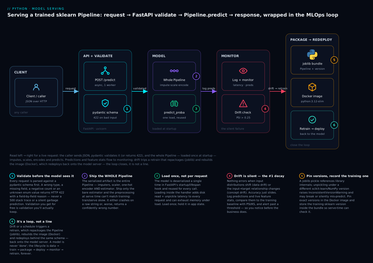
The six badges mark where deployments go wrong. Validate before the model (1) — a 422 at the boundary beats a crash or a garbage prediction. Ship the whole Pipeline (2) — the train/serve-skew point; only the estimator means silently wrong outputs. Load once at startup (3) — per-request loading is the classic latency killer. Drift is silent (4) — the failure with no exception, caught only by monitoring. Pin versions (5) — the joblib/sklearn version trap that corrupts predictions across a minor bump. And close the loop (6) — retraining repackages and redeploys back onto the model server, because the lifecycle is a wheel, not a line.
| Lifecycle stage | What happens | This lesson’s tool |
|---|---|---|
| Data | Collect, version, split | DVC; train_test_split |
| Train | Fit the Pipeline, evaluate | scikit-learn Pipeline, metrics |
| Package | Serialize the whole Pipeline | joblib.dump (+ version metadata) |
| Deploy | Serve behind an API, in a container | FastAPI + uvicorn + Docker |
| Monitor | Log predictions, watch drift/latency | logging, PSI/KS, alerting |
| Retrain | Triggered by drift or schedule → back to Train | scheduled + drift-triggered |
The honest tooling map
You can hand-build all of this — and understanding it by hand, as you just did, is why you can now evaluate the tools instead of cargo-culting them. But at scale, platforms package these concerns. The honest guidance: start simple (FastAPI + Docker + a bit of monitoring), and adopt a heavier tool only when a specific pain justifies its cost and lock-in. A managed platform earns its price when you have many models, a real serving scale, compliance requirements, or a team that shouldn’t be running Kubernetes by hand.
| Tool / platform | Layer | Earns its cost when |
|---|---|---|
| FastAPI + Docker | Serving (DIY) | Almost always the right starting point; full control, no lock-in |
| BentoML | Packaging + serving | You want standardized model packaging & autoscaling without hand-rolling it |
| MLflow | Tracking + registry | Many experiments/models to track, compare, and stage |
| Seldon / KServe | Serving on Kubernetes | You’re already on K8s and need canary/shadow, autoscaling, many models |
| AWS SageMaker | End-to-end (AWS) | Deep on AWS; want managed training→registry→endpoints |
| GCP Vertex AI | End-to-end (GCP) | Deep on GCP; want managed pipelines + endpoints |
| Azure ML | End-to-end (Azure) | Deep on Azure; want managed lifecycle + governance |
A managed platform buys you autoscaling, built-in monitoring, one-click canaries, and compliance scaffolding — and charges you money, lock-in, and a learning curve. For one model at modest scale, FastAPI + Docker + a PSI check in a cron job is not a toy; it’s the correct, cheap answer. Reach for the platform when the pain is real, not because the diagram looks impressive.
Hands-on lab
You will take a trained Pipeline all the way to a running, validated, monitored service — the full deployment path in seven steps. Everything runs on the venv from the top of the lesson (scikit-learn fastapi uvicorn pydantic joblib httpx pandas installed). Work in one directory; every output below is real.
Step 1 — Train a Pipeline and joblib.dump the WHOLE thing. Create train.py:
import json, numpy as np, pandas as pd, sklearn, joblib
from sklearn.model_selection import train_test_split
from sklearn.compose import ColumnTransformer
from sklearn.pipeline import Pipeline
from sklearn.preprocessing import StandardScaler, OneHotEncoder
from sklearn.impute import SimpleImputer
from sklearn.linear_model import LogisticRegression
from sklearn.metrics import accuracy_score

def make_customers(n=1200, seed=0):
    rng = np.random.default_rng(seed)
    city = rng.choice(["Bengaluru", "Delhi", "Mumbai", "Chennai"], size=n)
    plan = rng.choice(["free", "pro", "enterprise"], size=n, p=[0.6, 0.3, 0.1])
    tenure  = rng.gamma(2.0, 12.0, size=n).round(1)
    monthly = rng.normal(800, 300, size=n).clip(50).round(2)
    logins  = rng.poisson(20, size=n).astype(float)
    signal = (0.9*(plan == "free") - 0.03*tenure - 0.04*logins
              + 0.0005*monthly + rng.normal(0, 0.5, size=n))
    churn = (signal > np.quantile(signal, 0.7)).astype(int)
    df = pd.DataFrame({"city": city, "plan": plan, "tenure_months": tenure,
                       "monthly_inr": monthly, "logins_30d": logins, "churn": churn})
    df.loc[rng.choice(n, 80, replace=False), "tenure_months"] = np.nan
    df.loc[rng.choice(n, 60, replace=False), "city"] = None
    return df

df = make_customers()
X, y = df.drop(columns="churn"), df["churn"]
Xtr, Xte, ytr, yte = train_test_split(X, y, test_size=0.25, random_state=0, stratify=y)

numeric, categorical = ["tenure_months", "monthly_inr", "logins_30d"], ["city", "plan"]
pre = ColumnTransformer([
    ("num", Pipeline([("impute", SimpleImputer(strategy="median")),
                      ("scale", StandardScaler())]), numeric),
    ("cat", Pipeline([("impute", SimpleImputer(strategy="most_frequent")),
                      ("onehot", OneHotEncoder(handle_unknown="ignore"))]), categorical)])
model = Pipeline([("pre", pre), ("clf", LogisticRegression(max_iter=1000))])
model.fit(Xtr, ytr)
print("test accuracy:", round(accuracy_score(yte, model.predict(Xte)), 3))

joblib.dump({"model": model, "sklearn_version": sklearn.__version__,
             "features": numeric + categorical, "trained_at": "2026-07-17"},
            "churn-pipeline.joblib")
json.dump({c: {"mean": float(Xtr[c].mean()), "std": float(Xtr[c].std())} for c in numeric},
          open("train-stats.json", "w"), indent=2)
print("dumped churn-pipeline.joblib + train-stats.json")
test accuracy: 0.807
dumped churn-pipeline.joblib + train-stats.json
What just happened: one fit learned the imputation medians, scaling stats, encoder categories and classifier weights, and joblib.dump froze the entire Pipeline — preprocessing and all — to a 4.4 KB file, alongside the training feature stats you’ll need for drift detection.
Step 2 — Build the FastAPI service. Create app.py with the lifespan loader, pydantic schemas, and endpoints exactly as shown in the serving section (the PredictRequest/PredictResponse models, the lifespan that loads the bundle once, and the /health, /predict, /predict/batch handlers). The key lines:
@asynccontextmanager
async def lifespan(app):
    b = joblib.load("churn-pipeline.joblib")
    STATE.update(model=b["model"], features=b["features"], version=b["sklearn_version"])
    yield
    STATE.clear()
What just happened: the model is deserialized exactly once, at startup, into STATE — never per request.
Step 3 — Test it in-process (no network) with TestClient. Create test_app.py:
from fastapi.testclient import TestClient
from app import app
with TestClient(app) as c:                       # 'with' runs lifespan -> model loads
    print("health:", c.get("/health").json())
    good = {"tenure_months": 2.0, "monthly_inr": 1500.0, "logins_30d": 3,
            "city": "Mumbai", "plan": "free"}
    print("valid :", c.post("/predict", json=good).status_code,
          c.post("/predict", json=good).json())
    bad = {"tenure_months": 2.0, "monthly_inr": 1500.0, "logins_30d": -3, "plan": "platinum"}
    r = c.post("/predict", json=bad)
    print("invalid:", r.status_code, "fields:",
          sorted(e["loc"][-1] for e in r.json()["detail"]))
health: {'status': 'ok', 'sklearn': '1.9.0'}
valid : 200 {'churn': True, 'churn_probability': 0.9938, 'model_version': '1.9.0'}
invalid: 422 fields: ['city', 'logins_30d', 'plan']
What just happened: the valid request produced a real prediction (0.9938); the malformed one was rejected with a 422 naming all three bad fields — and the model never ran on the garbage.
Step 4 — Run the real server and hit it with httpx. In one terminal:
uvicorn app:app --host 127.0.0.1 --port 8000
In another (client.py):
import httpx
BASE = "http://127.0.0.1:8000"
print(httpx.get(f"{BASE}/health").json())                       # {'status': 'ok', 'sklearn': '1.9.0'}
good = {"tenure_months": 2.0, "monthly_inr": 1500.0, "logins_30d": 3,
        "city": "Mumbai", "plan": "free"}
print(httpx.post(f"{BASE}/predict", json=good).json())          # {'churn': True, 'churn_probability': 0.9938, ...}
loyal = {"tenure_months": 60.0, "monthly_inr": 400.0, "logins_30d": 40,
         "city": "Delhi", "plan": "enterprise"}
print(httpx.post(f"{BASE}/predict", json=loyal).json())         # {'churn': False, 'churn_probability': 0.0, ...}
What just happened: over real HTTP, the high-risk customer scored 0.9938 (churn) and the loyal one ~0.0 (stay). Same artifact, same code path as training — no skew possible.
Step 5 — Prove the “ship the whole Pipeline” rule. Add to client.py a check that the bare estimator fails on raw input:
import joblib, pandas as pd
b = joblib.load("churn-pipeline.joblib")
raw = pd.DataFrame([good])[b["features"]]
print("full  :", round(float(b["model"].predict_proba(raw)[0, 1]), 4))     # 0.9938
try:
    b["model"].named_steps["clf"].predict_proba(raw)                        # bare estimator
except ValueError as e:
    print("bare  :", type(e).__name__, "-", str(e).splitlines()[0])
full  : 0.9938
bare  : ValueError - could not convert string to float: 'Mumbai'
What just happened: the full Pipeline predicts; the bare estimator chokes on the raw string "Mumbai" because the one-hot encoder it needs was left behind. Ship the whole Pipeline.
Step 6 — Write the Dockerfile. Create Dockerfile and requirements.txt exactly as in the containerizing section (pinned python:3.12-slim, deps layer first, copy the .joblib and app.py, non-root user, CMD ["uvicorn", "app:app", "--host", "0.0.0.0", "--port", "8000"]). Then:
docker build -t churn-api:1.0.0 .
docker run -p 8000:8000 churn-api:1.0.0     # same service, now in a reproducible container
What just happened: the service and its exact environment — pinned sklearn 1.9.0 and all — are now one immutable image that runs identically on any machine, closing the version-mismatch trap.
Step 7 — A tiny drift check. Create drift.py comparing a live batch’s feature stats to training:
import json, numpy as np
stats = json.load(open("train-stats.json"))
m, s = stats["monthly_inr"]["mean"], stats["monthly_inr"]["std"]

def psi(expected, actual, bins=10):
    edges = np.quantile(expected, np.linspace(0, 1, bins + 1)); edges[0], edges[-1] = -np.inf, np.inf
    e = np.clip(np.histogram(expected, edges)[0] / len(expected), 1e-6, None)
    a = np.clip(np.histogram(actual,   edges)[0] / len(actual),   1e-6, None)
    return float(np.sum((a - e) * np.log(a / e)))

rng = np.random.default_rng(7)
base = rng.normal(m, s, 900)
for name, live in [("stable", rng.normal(m, s, 300)), ("drifted", rng.normal(m*1.4, s, 300))]:
    v = psi(base, live); print(f"{name:8} PSI={v:.3f} -> {'ALERT' if v > 0.25 else 'OK'}")
stable   PSI=0.033 -> OK
drifted  PSI=1.311 -> ALERT
What just happened: the batch matching training scored PSI 0.033 (fine); the batch where prices jumped 40% scored 1.311 — a loud drift alert, produced with no labels and no model call, just by comparing input stats to the baseline you saved at training time. That check, run on a rolling window of real requests, is the difference between catching decay in a day and discovering it in a quarterly review.
You now have the whole path: a trained Pipeline serialized whole, served behind a validated FastAPI endpoint, tested in-process and over HTTP, proven skew-proof, containerized with a pinned environment, and watched for drift.
Common mistakes and troubleshooting
| Symptom / traceback | Cause | Fix |
|---|---|---|
InconsistentVersionWarning: Trying to unpickle ... from version 1.9.0 when using 1.10.0 |
Model loaded under a different scikit-learn than it was trained on | Pin exact versions in requirements.txt/Docker; record & check sklearn_version in the bundle |
| Predictions are subtly wrong, no error | Shipped only the estimator; preprocessing at serve time differs — train/serve skew | Serialize the whole Pipeline; never rebuild preprocessing by hand |
ValueError: could not convert string to float: 'Mumbai' at predict |
Raw categorical reached a bare estimator (encoder was left behind) | Ship the Pipeline so the encoder runs before the estimator |
| Each request takes 200 ms+ and memory climbs | joblib.load() called inside the handler — model loaded per request |
Load once in lifespan/startup; hold it in app state |
422 Unprocessable Entity from the API |
Request body doesn’t match the pydantic schema (bad type/enum, missing field, out of range) | Fix the client payload; read detail[] — it names each bad field |
| Accuracy silently decayed over months; no alert ever fired | No monitoring — data/concept drift went undetected | Log predictions + feature stats; compute PSI/KS; alert past a threshold |
| Service freezes under load with a slow model | Blocking predict() called directly in an async def handler — event loop stalls |
Keep the handler def, or await loop.run_in_executor(None, fn) |
| Docker image is ~1 GB and slow to deploy | Used python:3.12 (full) or bloated layers |
python:3.12-slim; multi-stage build; --no-cache-dir |
FileNotFoundError: churn-pipeline.joblib in the container |
Model not COPYd into the image, or wrong WORKDIR |
Add COPY *.joblib .; verify the path relative to WORKDIR |
| Model path / secret hardcoded; breaks across environments | Config baked into code | Read from env vars / config; mount or fetch the model at boot |
ValueError: X has 5 features, but ... expecting 10 |
Fed the estimator raw columns, or wrong column order/count | Rebuild the DataFrame in the trained feature order; let the Pipeline transform |
| Prediction differs for the same input as a float vs int | dtype mismatch at the boundary (e.g. logins as "3" string or wrong dtype) |
Type it in pydantic (int/float); the schema coerces and validates |
AttributeError: Can't get attribute '...' on joblib.load |
Custom class/function not importable at load time (e.g. a FunctionTransformer referencing a local func) |
Make custom code importable (same module path) in the serving env |
Three of these cost the most hours and deserve extra words.
1. The version trap corrupts silently. A model pickled with scikit-learn 1.9 and loaded under 1.10 may not crash — it may load and return wrong probabilities, which is far worse than a clean failure because nothing tells you. The warning literally says “invalid results.” Your only real defence is to make the serving environment identical to training: pin scikit-learn, numpy, and scipy to exact versions in a container, and store the training version inside the artifact so the service can refuse (or scream) on a mismatch. This is the single strongest argument for containerizing model services.
2. Shipping the estimator instead of the Pipeline is the skew factory. It feels natural — “the model is the classifier” — but the preprocessing is part of the model. Detached, the serving code has to reproduce imputation, scaling, and encoding by hand, and any tiny discrepancy (unscaled inputs, a different one-hot order, a different fill value) produces confident, wrong predictions with no error. You saw a hand-coded input turn 0.9938 into 1.0. Serialize the whole Pipeline, always; then a single pipeline.predict() at serve time reruns the exact training transforms and skew is structurally impossible — the same guarantee the Pipeline gave you against leakage in training.
3. No monitoring means nobody notices decay. This is the quiet killer. Serialization and serving fail loudly; drift fails silently. The service returns 200s, latency is flat, and the model’s accuracy slides for months because the world moved and the model didn’t. There is no exception to catch — the absence of monitoring is the bug. Log every prediction’s inputs and outputs, compute a cheap drift signal (PSI on key features) on a rolling window, watch live accuracy against labels as they arrive, and alert on thresholds. The PSI check is a few lines; the cost of not having it is a model that “works” and quietly loses money.
Cheat-sheet
| Task | Code |
|---|---|
| Serialize the whole Pipeline | joblib.dump(pipeline, "model.joblib") |
| Serialize with metadata | joblib.dump({"model": p, "sklearn_version": v, "features": cols}, path) |
| Load a model | bundle = joblib.load("model.joblib") |
| Compress the artifact | joblib.dump(obj, path, compress=3) |
| Check version on load | if bundle["sklearn_version"] != sklearn.__version__: warn(...) |
| Convert to ONNX | to_onnx(model, X.astype("float32")) |
| pydantic request schema | class Req(BaseModel): x: float = Field(..., ge=0) |
| Restrict to an enum | plan: Literal["free", "pro", "enterprise"] |
| FastAPI app + lifespan | app = FastAPI(lifespan=lifespan) |
| Load model once at startup | @asynccontextmanager async def lifespan(app): STATE["m"]=joblib.load(...); yield |
| Prediction endpoint | @app.post("/predict", response_model=Resp) def predict(req: Req): ... |
| Return a specific error | raise HTTPException(status_code=503, detail="model not loaded") |
| Batch endpoint | def predict_batch(reqs: list[Req]): ... |
| Run the server | uvicorn app:app --host 0.0.0.0 --port 8000 |
| Hit it | httpx.post("http://localhost:8000/predict", json=payload) |
| Test in-process (CI) | with TestClient(app) as c: c.post("/predict", json=payload) |
| Offload a slow model | await loop.run_in_executor(None, lambda: model.predict(X)) |
| Interactive docs | visit http://localhost:8000/docs |
| Dockerfile base | FROM python:3.12-slim (never alpine for ML) |
| Docker start command | CMD ["uvicorn", "app:app", "--host", "0.0.0.0", "--port", "8000"] |
| Build & run image | docker build -t api:1.0 . && docker run -p 8000:8000 api:1.0 |
| Register a model (MLflow) | mlflow.sklearn.log_model(model, name="m", registered_model_name="churn") |
| PSI drift score | np.sum((a - e) * np.log(a / e)) over binned proportions |
| Drift alert threshold | PSI < 0.1 OK · 0.1–0.25 watch · > 0.25 alert |
| The rule | Ship the whole Pipeline, load once, validate every input, watch for drift |
Interview and exam questions
Q: Why serialize the whole Pipeline instead of just the trained estimator?
A: Because the preprocessing is part of the model. The estimator was trained on imputed, scaled, one-hot-encoded features; at serving time it must receive inputs shaped identically. Ship only the estimator and the serving code has to reproduce the preprocessing by hand, and any discrepancy causes train/serve skew — the model gets differently-shaped inputs and predicts garbage, sometimes crashing (a raw string reaches an estimator: ValueError: could not convert string to float), sometimes silently wrong (a hand-built unscaled input turned a correct 0.9938 into 1.0). Serialize the whole Pipeline and a single pipeline.predict() reruns the exact training transforms; skew becomes structurally impossible.
Q: What are the two big traps with pickle/joblib, and how do you mitigate each?
A: (1) Arbitrary code execution — unpickling runs code, so a malicious file can do anything; mitigate by only loading artifacts you produced, over authenticated channels, with checksums, and prefer ONNX for untrusted input. (2) Version fragility — a model pickled under scikit-learn 1.9 can fail or, worse, silently mis-predict under 1.10 (sklearn even warns: “invalid results”); mitigate by pinning exact scikit-learn/numpy/scipy versions in a container and recording the training version in the bundle to check on load. joblib fixes neither trap — it’s pickle underneath — it only makes large-array storage efficient.
Q: Why load the model at startup instead of inside the request handler?
A: joblib.load() reads from disk and reconstructs a whole object graph — doing it per request adds tens to hundreds of milliseconds to every call and can exhaust memory under load. Load it once when the process starts (FastAPI’s lifespan/startup hook) and hold it in application state, so every request reuses the one in-memory model. Loading per request is the single most common ML-serving performance bug.
Q: What does pydantic give you in a serving API, and what is a 422?
A: pydantic validates every request against a declared schema (types, ranges via Field(ge=…), enums via Literal, required fields) before the model runs. A request that doesn’t match gets an automatic HTTP 422 Unprocessable Entity with a field-by-field explanation — e.g. a negative logins_30d, a missing city, and a plan outside the allowed set all reported at once. This means garbage is rejected at the boundary with a machine-readable reason, instead of crashing the model or silently predicting on nonsense. You write type hints; you get a validation layer and interactive docs for free.
Q: Explain data drift vs concept drift. Which can you detect without labels?
A: Data drift (covariate shift) is when the input distribution P(X) changes — the model’s input→output mapping is still valid, but it’s seeing unfamiliar inputs (prices rise 40%, a new city appears). Concept drift is when the relationship P(y|X) changes — the same inputs now mean something different (a recession changes who churns). You can detect data drift without any labels by comparing live input statistics to the training baseline (e.g. PSI, KS test) — in a demo, a 40% price shift produced PSI 1.311 vs 0.033 for a stable batch. Concept drift generally needs the true outcomes to see that accuracy has dropped, and those labels usually lag.
Q: Why is a container the right way to ship a model service?
A: A container packages the application with its exact environment — pinned Python and library versions, the model file, the code — into one immutable image that runs identically everywhere. That directly solves the version-mismatch trap: the serving scikit-learn is byte-for-byte the one the model was trained with, so predictions can’t be silently corrupted by a minor-version bump. It also makes deploys reproducible and rollbacks trivial (redeploy the previous image). Use python:3.12-slim (not full, not alpine — musl breaks NumPy/SciPy wheels), install deps in a cached layer before copying code, and run as non-root.
Q: What is shadow deployment and when would you use it? A: Shadow (mirror) deployment runs a new model on live traffic in parallel with the current one, but its predictions are not served to users — you compare them to the incumbent (or to actual outcomes) with zero user risk, then promote once you trust it. It’s the safest strategy for ML because a model’s real quality can only be judged against live data, and shadow lets you get that judgment before committing a single user to it. Contrast with canary (serve to a small, growing traffic slice) and blue-green (flip 100% at once with instant rollback).
Q: You have an async def FastAPI handler and a slow model. What’s the bug and the fix?
A: The bug is that model.predict() is synchronous, CPU-bound code; calling it directly in an async def handler blocks the event loop, stalling every other in-flight request behind it. The fix is either to define the handler as plain def (FastAPI runs sync handlers in a threadpool automatically) or, in an async handler, offload the blocking call with await loop.run_in_executor(None, lambda: model.predict(X)), which pushes the CPU work to a threadpool and keeps the loop free to serve other requests.
Q (coding): Sketch a minimal FastAPI /predict endpoint that loads a joblib Pipeline once and validates input.
A:
from contextlib import asynccontextmanager
from fastapi import FastAPI
from pydantic import BaseModel, Field
import joblib, pandas as pd

STATE = {}
@asynccontextmanager
async def lifespan(app):
    STATE["m"] = joblib.load("model.joblib")["model"]   # load ONCE
    yield
app = FastAPI(lifespan=lifespan)

class Req(BaseModel):
    tenure_months: float = Field(..., ge=0)
    plan: str

@app.post("/predict")
def predict(req: Req):                                   # def -> threadpool, non-blocking
    X = pd.DataFrame([req.model_dump()])
    return {"proba": float(STATE["m"].predict_proba(X)[0, 1])}
The model loads once in lifespan, pydantic validates every request (bad input → 422 automatically), and a plain def handler keeps the sync predict off the event loop.
Q: How does the MLOps lifecycle differ from “train and deploy”? A: “Train and deploy” treats deployment as the finish line; MLOps treats it as one arc of a loop: data → train → package → deploy → monitor → retrain → (back to train). The addition is everything after deploy — monitoring for drift and decay, and retraining (scheduled and/or drift-triggered) that feeds a new model back into packaging and deployment. A model is never “done”; it is currently deployed and being watched for the day the world drifts far enough that it must be replaced. Skipping the monitor→retrain half is why models that launched at 0.81 accuracy quietly degrade in production.
Q: What would you log on every prediction, and why? A: The input features, the prediction (and probability), the model version, and the latency. Inputs + outputs let you compute drift (compare live feature stats to the training baseline) and debug specific bad predictions; the model version ties each prediction to a registered artifact for traceability; latency feeds SLA/performance monitoring (p50/p95/p99). Guard PII — hash or drop sensitive fields and respect retention. Without this logging you have no way to detect the silent decay that is the number-one production ML failure.
Q: When does a managed ML platform (SageMaker/Vertex/Azure ML) earn its cost over FastAPI + Docker? A: When a specific pain justifies the price and lock-in: many models to serve and govern, real serving scale needing autoscaling, built-in monitoring and one-click canary/shadow, compliance/audit requirements, or a team that shouldn’t hand-run Kubernetes. For one model at modest scale, FastAPI + Docker + a PSI check in a cron job is the correct, cheap answer — not a toy. Start simple; adopt the platform when the pain is real, not because it looks impressive on an architecture diagram.
Key takeaways
- A model in a notebook earns nothing — deployment is the value. The gap between
model.fit()and something a product can call has three parts: serialization (survive leaving memory), serving (something calls.predict()), and monitoring (know it still works). Get any one wrong and the model’s value stays locked inside it. - Serialize with joblib, but respect its two traps. joblib is the sklearn default (efficient on big arrays, optional compression), but it’s pickle underneath: it can execute arbitrary code on load (only load your own artifacts) and is version-fragile (a model from sklearn 1.9 can silently mis-predict on 1.10 — “invalid results”). Pin exact versions and record the training version in the bundle. Use ONNX when you need cross-language, edge, or untrusted-input serving.
- Ship the WHOLE Pipeline, never the bare estimator — this is the cardinal rule. Preprocessing is part of the model. Detach it and you get train/serve skew: a raw string crashes the estimator, or a hand-built input silently turns a correct 0.9938 into a wrong 1.0. Serialize the whole
Pipelineand a singlepredict()reruns the exact training transforms — skew becomes impossible, just as it did for leakage in training. - Serve with FastAPI: validate every input, load the model once. pydantic schemas reject malformed requests with an automatic, field-by-field 422 before the model runs; loading the model at startup (not per request) is the difference between a fast service and a slow, memory-thrashing one. Return proper status codes (200/422/503/500), batch when you can, and keep slow models off the async event loop with
run_in_executor. - Containerize to pin the environment. A Docker image ships the model with its exact, pinned dependencies, which is the real fix for the version-mismatch trap. Use
python:3.12-slim(never alpine for ML), install deps in a cached layer before copying code, run as non-root, and watch image size — it’s what you pull on every deploy. - Monitoring is the part everyone skips and the #1 production failure. A deployed model decays silently — no exception, no error, just accuracy sliding as the world moves. Data drift (input distribution shifts, detectable without labels via PSI/KS — 1.311 vs 0.033 in the demo) and concept drift (the input→target relationship changes, needs labels) both degrade the model quietly. Log predictions, compare live stats to the training baseline, and alert on thresholds.
- Deploy safely and retrain on a trigger. Never flip 100% of traffic to an unproven model: canary a small slice, blue-green for instant rollback, or shadow to score live traffic risk-free before serving it. Retrain on a schedule and/or when drift crosses a threshold — a deployed model is a depreciating asset.
- The MLOps lifecycle is a loop, not a line. Data → train → package (joblib) → deploy (Docker) → monitor (drift) → retrain → and around again. Deployment is not the end; it’s one turn of a wheel that never stops. Start simple with FastAPI + Docker + a drift check, and reach for a managed platform (MLflow, BentoML, Seldon/KServe, SageMaker/Vertex/Azure ML) only when a real pain — scale, many models, compliance — justifies its cost and lock-in.
This is the deployment chapter of the machine-learning arc: you can now take any trained scikit-learn Pipeline, freeze it whole with joblib, serve it behind a validated FastAPI endpoint that loads it once and rejects garbage with a 422, package it in a reproducible container, and — the part that separates a demo from a product — watch it for the drift that would otherwise degrade it in silence. The habit from the preprocessing lesson (everything inside one Pipeline) is exactly what makes serving skew-proof here; the honest metrics from train/test split and evaluation are what your monitoring compares against; and the structured logging from logging and debugging is what feeds every drift check. A model is never finished — it is deployed, monitored, and, when the world moves far enough, retrained and shipped again.