You have assembled the toolkit one piece at a time: the train/test split and the metrics that refuse to lie, the algorithm zoo — linear models, SVMs, trees, kNN, and cross-validation with hyperparameter tuning. This lesson plays the whole piece. We take one real problem — which subscribers are about to churn? — and carry it end to end: frame → acquire + EDA → split (seal the test) → preprocess in a Pipeline → train and compare → tune → evaluate honestly → interpret → package → serve → reproduce. Every number below is executed on Python 3.12.3 with scikit-learn 1.9.0, pandas 3.0.3, NumPy 2.5.1, SciPy 1.18.0, matplotlib 3.11.0, joblib 1.5.3, FastAPI 0.139.2 and pydantic 2.13.4, and the whole thing is seeded so it re-runs to the same answer.
A capstone is not about learning more methods; it is about judgement and discipline — the order you do things in, the checks that catch a wrong answer before it ships, and the one habit (seal the test set, and never leak into it) that separates a model you can trust from a demo that memorised its own answers. Our through-line is a single sentence, the same one the metrics lesson burned in: scikit-learn will almost never raise on a leaky, mis-measured, or overfit model — it hands you a clean, high-looking score that is quietly wrong. Our defence is the workflow and the discipline baked into each step. We will hit the traps on purpose. Our headline metric — accuracy — will say our do-nothing baseline is 76% good; the correct read says that baseline catches exactly zero of the customers we exist to save. The gap between those two is this lesson.
Why this matters
Most ML tutorials hand you load_iris(), call .fit(), print 0.97, and stop. Real ML work is the opposite shape: the model is maybe 5% of the effort and almost never where projects fail. Projects fail because someone scaled the features before splitting and leaked the test set into training; because they optimised accuracy on a 24%-positive problem and shipped a model that never predicts the positive class; because they tuned against the test set until it stopped being a test set; because they saved the model but not the preprocessing, so the API fed raw strings to something that expected scaled numbers. None of those raise an exception. All of them produce a confident, plausible, wrong number that reaches a stakeholder.
The job, then, is a pipeline of verbs done in a specific order, and the order is load-bearing. You cannot preprocess before you split (that leaks). You cannot compare models before you have a leakage-proof pipeline (the comparison is contaminated). You cannot report a score you tuned against (it is optimistic by construction). And you cannot pick a decision threshold before you know the cost of the two ways to be wrong (0.50 is a default, not an answer). Two junctions decide whether the final number is true. The first is the split: seal the test set the moment it is created and let a Pipeline own every fit, or leakage silently inflates everything downstream. The second is evaluation: on imbalanced data, accuracy is a liar, and only the confusion matrix, the right metric, and a real baseline tell you what the model actually does. We spend most of our care at those two junctions.
Our project is customer churn for a subscription business. Each row is one customer; the label churned is 1 if they left. It is a binary classification problem with class imbalance (~24% churn) and a couple of realistic data issues — which is exactly why every Phase-5 lesson matters here: the imbalance makes the metric choice decisive, the messy CSV makes the pipeline decisive, and the business cost of a lost customer makes the threshold decisive. By the end we have a joblib file holding the whole fitted pipeline and a FastAPI service that scores a customer in one HTTP call — tested, seeded, and reproducible by anyone who clones the repo.
Frame the problem — business question to ML task to metric
Before a single read_csv, write down what you are actually deciding, because the decision picks the metric, and the wrong metric optimises the wrong thing all the way to production. “Build a churn model” is not a task; it is a way to spend a month and ship something nobody can act on. A framed ML problem names the business question, the unit of prediction, the label, and — the part everyone skips — the relative cost of the two errors.
| Vague ask | Framed, answerable ML problem |
|---|---|
| “Do something about churn” | For each active customer, predict P(churn in the next cycle) so retention can call the top-risk list. |
| “Build a churn model” | Binary classifier; unit = one customer; label = churned; features = plan, tenure, usage, billing, support. |
| “Make it accurate” | Maximise recall on churners at an acceptable precision, because a missed churner costs far more than a wasted call. |
| “Is the model good?” | Beat a DummyClassifier on PR-AUC, and quote the confusion matrix at the threshold set by business cost. |
The last two rows are where the money is. This is a churn problem, so the two ways to be wrong are not symmetric. A false negative — we predict “stays,” the customer leaves — costs a whole customer’s future value. A false positive — we predict “churns,” they would have stayed — costs one retention offer (a discount, a call). Losing a customer is worth many retention offers, so we price a miss at roughly 4× a false alarm. That single ratio decides everything downstream: it tells us to favour recall over precision, to select models on PR-AUC rather than accuracy, and to move the decision threshold below the default 0.50 on purpose.
Spell the four outcomes out in the language of the business, with the cost attached, because this table is the objective function — everything the model does is a bet against it:
| Model says | Reality | Outcome | Business meaning | Cost |
|---|---|---|---|---|
| churn | churns | True positive | flagged a real churner; retention calls, may save them | 0 (the win) |
| stay | churns | False negative | missed a churner; they leave unnoticed | high (a lost customer ≈ 4 units) |
| churn | stays | False positive | flagged a loyal customer; a wasted retention offer | low (1 unit) |
| stay | stays | True negative | correctly left alone | 0 |
The asymmetry in that last column is the entire reason accuracy is the wrong lens: accuracy treats a false negative and a false positive as equally bad (both “one wrong”), while the business treats a false negative as four times worse. A metric that can’t see the difference will happily optimise toward the cheap-looking, expensive-in-reality answer. We encode the 4:1 ratio explicitly and let it drive model selection and the threshold.
Where does 4:1 come from? Ground it in money. Say a churned customer’s remaining lifetime value is roughly £400, a successful retention save recovers a fair fraction of that, and a retention offer (a call plus a discount) costs about £100 whether or not it lands. Then missing a churner risks the £400; a false alarm burns £100. The ratio of the two costs — not their exact values — is what sets the threshold, so you do not need a precise LTV model to start; a defensible order-of-magnitude ratio already beats the accidental 1:1 that accuracy assumes. As you learn the real numbers, you update the ratio and re-derive the threshold — the framework stays, the constant sharpens. This is the expected-value view of a classifier: every prediction is a bet, and the threshold is where the expected cost of “call them” drops below the expected cost of “let them go.”
| Business reality | ML consequence |
|---|---|
| A missed churner costs ≫ a wasted retention offer | optimise recall / PR-AUC, not accuracy; threshold below 0.50 |
| Only ~24% of customers churn (imbalance) | accuracy is dominated by the majority; a do-nothing model looks “good” |
| Retention has finite call capacity | precision still matters — an all-positive model is useless; hence PR-AUC, not raw recall |
| The model informs a repeated, reversible action (a call) | a directional score is actionable; we don’t need a randomized trial to start |
Picking the metric to match the cost is the single most consequential decision in the project, and it happens before any modelling. Here is the whole lifecycle we are about to walk, with the two discipline points marked:
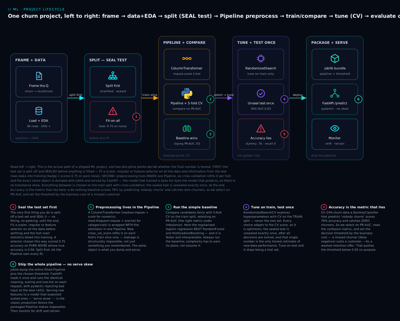
Read it left to right. The verbs in the middle are cheap; the two red discipline points — seal the test set (badge 1) and ship the whole pipeline (badge 6) — are where a project is quietly won or lost, and the amber “accuracy lies” node (badge 5) is where an imbalanced problem fools the unwary. We will touch every badge with real code and real output.
Our dataset is a synthetic-but-realistic customer table. Each row is one customer; the columns are:
| Column | Meant to be | What it carries / the issue |
|---|---|---|
customer_id |
string id | dropped before modelling — an id is not a feature |
tenure_months |
int 0–72 | months as a customer; strong (nonlinear) churn signal |
contract |
month-to-month / one-year / two-year | the dominant driver — short contracts churn |
payment_method |
4 categories | electronic-check cohort churns more |
internet_service |
fiber / dsl / no-internet | dirty: case + whitespace noise from three source systems |
paperless_billing |
yes / no | weak signal |
senior |
0 / 1 | weak signal |
add_on_services |
int 0–6 | more add-ons ⇒ stickier (protective) |
support_tickets |
int | frustration signal; 60 missing (logging gap) |
monthly_charges |
float | price sensitivity; one impossible −999 (data slip) |
total_charges |
float | arrives as text with blanks for brand-new customers (the classic bug) |
churned |
0 / 1 | the label; ~24% positive |
Two of those issues — total_charges typed as text, and internet_service spelled nine ways — are the kind that silently poison a model if you don’t catch them. We will.
Acquire and explore (EDA)
Load the data and look before you leap. The first two lines you run on any dataset are .dtypes and a class-balance check, because a wrong dtype poisons every downstream statistic and the class balance decides your entire metric strategy. (The mechanics of EDA are the subject of the data-analysis capstone; here we run it in service of a modelling decision.)
import pandas as pd
raw = pd.read_csv("data/churn.csv")
print("shape:", raw.shape, "| exact duplicate rows:", int(raw.duplicated().sum()))
print(raw.dtypes.to_string())
shape: (8012, 12) | exact duplicate rows: 12
customer_id           str
tenure_months       int64
...
support_tickets   float64
monthly_charges   float64
total_charges      object     <-- should be a number!
churned             int64
Two diagnostics fire immediately. There are 12 exact duplicate rows (a logging retry double-wrote them) — dedupe before counting anything, or every rate is inflated. And total_charges came in as object (text), not a number, because brand-new customers have a blank " " billed-nothing cell and one text value in a column forces the whole column to strings. A numeric column arriving as object is the single most common data bug there is, and .dtypes catches it in ten seconds. We dedupe (8012 → 8000 rows) and defer the dtype fix to the cleaning step.
Now the class balance — the number that dictates our metric strategy:
df = raw.drop_duplicates().reset_index(drop=True)
print("class balance:", df["churned"].value_counts(normalize=True).round(3).to_dict())
class balance: {0: 0.757, 1: 0.243}
24.3% churn. This is the whole reason accuracy is about to lie: a model that predicts “nobody churns” for every customer is right 75.7% of the time and useless. Hold that number — 0.757 — it is the accuracy our do-nothing baseline will score, and the bar accuracy dishonestly clears.
EDA’s real job here is to find the signal and confirm our suspicions about the drivers, so we cut churn by every categorical. We look only at the training data in a moment (never explore the test set), but the aggregate shape is already instructive:
for col in ["contract", "internet_service", "payment_method"]:
    r = df.groupby(col)["churned"].agg(["size", "mean"]).round(3)
    print(f"\n[{col}]\n{r.to_string()}")
[contract]
                   size   mean
month-to-month     3506  0.382
one-year           1677  0.096
two-year           1217  0.044

[internet_service]
             size   mean
dsl          2433  0.157
fiber        2817  0.373
no-internet  1150  0.105

[payment_method]
                  size   mean
electronic-check  2246  0.271
credit-card       1507  0.220
...
The signal is loud and realistic. Contract dominates: month-to-month churns at 38%, two-year at 4% — a 9× spread. Fiber customers churn far more than DSL or no-internet (a price/reliability cohort). Electronic-check payers churn most. This is where you form hypotheses; the model will confirm them quantitatively in the interpretation step. Cut by tenure and by the numeric correlations too:
print(df[["tenure_months","monthly_charges","support_tickets"]]
      .corrwith(df["churned"]).round(3).to_string())
monthly_charges    0.225
support_tickets    0.125
tenure_months     -0.125
monthly_charges correlates positively (pricey plans churn), support_tickets positively (frustration), tenure_months negatively (loyalty). But note tenure’s linear correlation looks weak (−0.125) even though it is a strong driver — because the real tenure effect is nonlinear (a churn cliff in the first six months that flattens later), and Pearson correlation only sees the straight-line part. This is a preview of a key lesson: linear correlation understates nonlinear signal, which is why we let the model — and later permutation importance — find the real importance rather than trusting a correlation table.
| EDA move | What we ran | What it told us |
|---|---|---|
| dtype audit | df.dtypes |
total_charges is text — a hidden numeric-parsing bug |
| duplicate check | df.duplicated().sum() |
12 phantom rows to drop before counting |
| class balance | value_counts(normalize=True) |
24.3% churn ⇒ accuracy will lie; select on PR-AUC |
| categorical cuts | groupby(col)["churned"].mean() |
contract, internet, payment carry the signal |
| numeric correlation | corrwith(y) |
monthly/tickets/tenure matter; tenure’s effect is nonlinear |
The output of EDA is not a chart — it is a short list of expectations to hold the model accountable to: contract, monthly charges, tenure and tickets should dominate; paperless and total_charges should barely matter. If the fitted model disagrees wildly, one of us is wrong, and that is a bug worth finding.
Split first — seal the test set (and the leakage trap)
This is the golden rule, and it is the first thing you do to the data, before any cleaning that learns a statistic and before any modelling: carve off a test set and seal it. The test set exists to answer one question — “how will this model do on customers it has never seen?” — and it can only answer honestly if nothing about it, not one median, not one scaler mean, not one category list, ever influenced training.
from sklearn.model_selection import train_test_split

X = df[FEATURES].copy()          # 10 feature columns, id and label removed
y = df["churned"].astype(int)
X_train, X_test, y_train, y_test = train_test_split(
    X, y, test_size=0.20, stratify=y, random_state=42)   # SEAL X_test/y_test now
print(f"train={X_train.shape}  test={X_test.shape}  "
      f"train churn={y_train.mean():.3f}  test churn={y_test.mean():.3f}")
train=(6400, 10) test=(1600, 10) train churn=0.243 test churn=0.243
Two arguments make the split honest. stratify=y keeps the 24.3% churn rate identical in both halves — on imbalanced data an unstratified split can hand you a test set with a wildly different positive rate, making the final score meaningless. random_state=42 makes the split reproducible, so your run matches this lesson’s exactly. From this line on, X_test and y_test are untouchable until the very end.
Why insist on stratification? Because random chance bites hardest exactly where the positives are scarce. With 24% churn and 1,600 test rows the law of large numbers mostly protects you, but drop to a 2%-positive fraud problem with a few hundred rows and an unstratified split can deal a fold with a handful of positives — or none — and a recall computed on two churners is noise, not a measurement. Stratifying costs nothing and removes that variance, so it is the default for every classification split and every cross-validation fold (StratifiedKFold, which we use throughout). The habit generalises: whenever a subgroup is both important and rare, make the split preserve its proportion rather than trusting the dice.
The leakage trap, demonstrated on pure noise
Why so strict? Because the most dangerous bug in ML is invisible: fit anything that learns from data — a scaler, an imputer, a feature selector — on the whole dataset before splitting, and information from the test rows leaks into training. Every downstream score inflates, and nothing warns you. Here is the canonical proof, on data with no signal at all:
import numpy as np
from sklearn.feature_selection import SelectKBest, f_classif
from sklearn.linear_model import LogisticRegression
from sklearn.pipeline import Pipeline
from sklearn.model_selection import cross_val_score, StratifiedKFold

rng = np.random.default_rng(0)
X_noise = rng.normal(size=(300, 5000))   # 5000 columns of PURE NOISE
y_rand  = rng.integers(0, 2, size=300)   # random labels — true accuracy is 0.50
cv = StratifiedKFold(5, shuffle=True, random_state=0)

# WRONG: pick the 20 "best" features using ALL rows (incl. the validation fold)
X_sel = SelectKBest(f_classif, k=20).fit_transform(X_noise, y_rand)
leaky = cross_val_score(LogisticRegression(max_iter=1000), X_sel, y_rand, cv=cv).mean()

# RIGHT: selection inside the Pipeline, refit on each fold's train slice only
pipe = Pipeline([("sel", SelectKBest(f_classif, k=20)),
                 ("clf", LogisticRegression(max_iter=1000))])
honest = cross_val_score(pipe, X_noise, y_rand, cv=cv).mean()
print(f"leaky  (select on ALL data): {leaky:.3f}")
print(f"honest (select in Pipeline): {honest:.3f}")
leaky  (select on ALL data): 0.750
honest (select in Pipeline): 0.537
Sit with that. The labels are coin flips — the true accuracy is 0.500. The honest pipeline reports 0.537 (chance, plus noise). The leaky version reports 0.750 — a “great” model, built on nothing, because the feature selector peeked at the validation rows’ labels when it chose which of 5000 noise columns to keep. If you have ever seen a model score suspiciously well in cross-validation and collapse in production, this is very often why.
| Leakage type | How it sneaks in | The fix |
|---|---|---|
| Preprocessing leakage | scaler/imputer/selector fit on all data before the split | fit inside a Pipeline; split first |
| Target leakage | a feature secretly built from the label (e.g. days_since_churn) |
audit every feature: could it exist before the label did? |
| Temporal leakage | shuffling a time series so the model trains on the future | split by time, not at random, for time-ordered data |
| Group leakage | the same customer/user in both train and test | GroupShuffleSplit on the entity id |
The lesson that outlasts the syntax: you do not avoid leakage by being careful — you avoid it by making it structurally impossible. That is the entire point of the Pipeline we build next. (The split-and-metrics lesson drills each leakage form; here we simply refuse to let it happen.)
Preprocess in a Pipeline — leakage-proof by construction
Our features are mixed: six numeric columns (some with holes, on wildly different scales) and four categorical columns (text). Different types need different preparation, and every preparation step learns a statistic from the data — the median to impute with, the mean/σ to scale by, the list of categories to encode. Each of those must be learned from the training slice only. The tool that guarantees this is a ColumnTransformer wrapped in a Pipeline.
First, the leakage-free cleaning that does not learn a statistic (so it can safely run on all rows): fix the text dtype, normalise the dirty category, and null the impossible value. Anything that does learn a statistic — imputing, scaling, encoding — we defer into the pipeline.
import numpy as np

def clean(raw: pd.DataFrame) -> pd.DataFrame:
    df = raw.drop_duplicates().reset_index(drop=True)
    df["total_charges"] = pd.to_numeric(df["total_charges"], errors="coerce")  # text -> NaN
    df["internet_service"] = df["internet_service"].str.strip().str.lower()    # 9 spellings -> 3
    df.loc[df["monthly_charges"] < 0, "monthly_charges"] = np.nan               # -999 slip -> NaN
    return df
After cleaning, the holes that remain are honest missing values to be imputed inside the pipeline:
NaN per feature: monthly_charges 1 total_charges 105 support_tickets 60
Each mess has a signature and a fix, and the discipline is to handle the kind of hole correctly rather than blindly fillna(0) everything:
| Data issue | How you catch it | Fix (and where it belongs) |
|---|---|---|
total_charges typed as text |
.dtypes shows object on a numeric column |
pd.to_numeric(errors="coerce") in clean() — blanks → NaN |
internet_service in 9 spellings |
value_counts() shows near-duplicate categories |
.str.strip().str.lower() in clean() — normalise before one-hot |
impossible monthly_charges = -999 |
.describe() shows a min below any real value |
domain rule → NaN in clean(), then impute in the pipeline |
| 12 duplicate rows | df.duplicated().sum() |
drop_duplicates() first — before any count |
60 missing support_tickets, 105 missing total_charges |
df.isna().sum() |
SimpleImputer inside the pipeline (fit on train only) |
The split in that last column is the whole point: clean() does only what is leakage-free — dtype fixes, category normalisation, nulling an impossible value — none of which learns a statistic from the data, so it can safely run on all rows. Anything that learns a fill value (the median for imputation) is deferred into the pipeline, where cross-validation refits it per fold. A tenure-0 customer’s total_charges is really 0, not the median; we let the imputer fill it because the alternative — a domain rule in clean() — would still be leakage-free, but keeping all imputation in one place (the pipeline) is the habit that never leaks. With only 105 such rows out of 8,000, the choice barely moves the result, and the discipline is worth more than the fractional accuracy.
Now the preprocessor. Numeric columns get median imputation (robust to the outliers we nulled) then standard scaling; categorical columns get most-frequent imputation then one-hot encoding with handle_unknown="ignore" so a category never seen in training can’t crash serving:
from sklearn.compose import ColumnTransformer
from sklearn.pipeline import Pipeline
from sklearn.impute import SimpleImputer
from sklearn.preprocessing import StandardScaler, OneHotEncoder

NUMERIC = ["tenure_months", "monthly_charges", "total_charges",
           "add_on_services", "support_tickets", "senior"]
CATEGORICAL = ["contract", "payment_method", "internet_service", "paperless_billing"]

def build_preprocessor() -> ColumnTransformer:
    numeric = Pipeline([("impute", SimpleImputer(strategy="median")),
                        ("scale", StandardScaler())])
    categorical = Pipeline([("impute", SimpleImputer(strategy="most_frequent")),
                           ("onehot", OneHotEncoder(handle_unknown="ignore"))])
    return ColumnTransformer([("num", numeric, NUMERIC),
                             ("cat", categorical, CATEGORICAL)])
| Column type | Steps | Why in this order, why in the pipeline |
|---|---|---|
| numeric | SimpleImputer(median) → StandardScaler |
impute first (a NaN has no z-score); median resists outliers; scaling helps the linear model, harms nothing |
| categorical | SimpleImputer(most_frequent) → OneHotEncoder |
fill the gap, then give each category its own 0/1 column so the model reads no fake order |
| unseen category at serve time | handle_unknown="ignore" |
encode it as all-zeros instead of raising — the API stays up |
| any column you forget to list | ColumnTransformer default remainder="drop" |
silently dropped — a real gotcha; list every column or set remainder="passthrough" |
The magic is what happens when this preprocessor rides inside a full pipeline through cross-validation: on every fold, .fit() learns the median, the mean/σ and the category list from that fold’s training rows only, then merely applies them to the held-out rows. Leakage is not something you remember to avoid — it is impossible by construction. And because the very same fitted object is what we later joblib.dump and serve, the API runs the identical transforms. This one design decision closes both discipline points on the diagram at once. (The mechanics of ColumnTransformer and each transformer are the subject of the preprocessing material in the algorithms lesson.)
Train and fairly compare — baseline, linear, forest, boosting
Now we compare candidates, each one preprocessing + estimator in a single pipeline, with 5-fold cross-validation on the training set only. We include a DummyClassifier as the honesty anchor, a LogisticRegression as the interpretable baseline, and two ensembles — RandomForestClassifier and HistGradientBoostingClassifier — because tree ensembles are the usual champions on tabular data. All three real models get class_weight="balanced" to counter the imbalance.
from sklearn.dummy import DummyClassifier
from sklearn.ensemble import RandomForestClassifier, HistGradientBoostingClassifier
from sklearn.model_selection import cross_validate, StratifiedKFold
from sklearn.metrics import make_scorer, f1_score, recall_score, precision_score

CV = StratifiedKFold(n_splits=5, shuffle=True, random_state=42)

def candidates():
    pre = build_preprocessor
    return {
        "dummy":  Pipeline([("pre", pre()), ("clf", DummyClassifier(strategy="most_frequent"))]),
        "logreg": Pipeline([("pre", pre()), ("clf", LogisticRegression(
                     solver="saga", max_iter=5000, class_weight="balanced", random_state=42))]),
        "rf":     Pipeline([("pre", pre()), ("clf", RandomForestClassifier(
                     n_estimators=400, class_weight="balanced", random_state=42, n_jobs=-1))]),
        "histgb": Pipeline([("pre", pre()), ("clf", HistGradientBoostingClassifier(
                     class_weight="balanced", random_state=42))]),
    }

scoring = {"roc_auc": "roc_auc", "pr_auc": "average_precision",
           "f1": make_scorer(f1_score, zero_division=0),
           "recall": make_scorer(recall_score, zero_division=0),
           "precision": make_scorer(precision_score, zero_division=0)}
We select on PR-AUC (average precision), the right summary metric under imbalance, and report ROC-AUC, F1, recall and precision alongside. Running cross_validate on each pipeline and averaging the folds gives the comparison table:
        roc_auc  pr_auc  pr_auc_std      f1  recall  precision
dummy    0.5000  0.2428      0.0003  0.0000  0.0000     0.0000
logreg   0.8331  0.6340      0.0151  0.5936  0.7703     0.4829
rf       0.8113  0.5955      0.0143  0.5693  0.6042     0.5385
histgb   0.8245  0.6228      0.0163  0.6034  0.7156     0.5219
Read that carefully, because it contains a lesson worth more than any single model. The regularised logistic regression won — PR-AUC 0.634, ahead of HistGradientBoosting’s 0.623 and RandomForest’s 0.596. The gradient booster, the odds-on favourite for tabular data, came second. And the DummyClassifier posts PR-AUC 0.243 (exactly the base rate) with recall and F1 of zero — it never predicts churn, which is precisely what makes its accuracy dishonest.
| Model | CV PR-AUC | Verdict |
|---|---|---|
DummyClassifier |
0.243 | the honesty floor — any real model must clear it |
LogisticRegression (elasticnet) |
0.634 | winner: best PR-AUC, fastest, and interpretable |
HistGradientBoostingClassifier |
0.623 | excellent, a whisker behind — would win on many datasets |
RandomForestClassifier |
0.596 | solid, third here |
This is the run-the-baseline lesson, and it is one of the most valuable in applied ML: complexity has to earn its place, not assume it. A one-hot logistic regression is fast to train, trivial to serve, and directly interpretable, and here it matches or beats two ensembles that are slower and opaque. Practitioners waste enormous effort reaching for gradient boosting when a regularised linear model would have tied it. Always run the simple baseline; make the fancy model prove it is worth the cost. Here it isn’t, so we take logistic regression forward — and get interpretability for free.
The four candidates span the trade-off space on purpose, and knowing why each behaves as it does is the reusable skill (the full treatment is the algorithms lesson):
| Model | How it decides | Needs scaling? | Interpretable? | Reach for it when |
|---|---|---|---|---|
DummyClassifier |
predicts the majority (or a fixed rule) | no | trivially | always — as the honesty baseline, never to ship |
LogisticRegression |
weighted sum of features → sigmoid | yes (regularised) | yes (coefficients/odds) | a strong, fast, explainable baseline; roughly linear signal |
RandomForestClassifier |
vote of many de-correlated trees | no (scale-invariant) | partly (importances) | nonlinear signal, interactions, minimal tuning |
HistGradientBoostingClassifier |
trees fit sequentially to residuals | no | partly (importances) | the usual tabular champion; squeezes out interactions |
Note the “needs scaling” column: the tree models are scale-invariant, so the StandardScaler in our pipeline neither helps nor hurts them — but it is essential for the logistic regression, whose regularisation penalises large coefficients and so is sensitive to feature scale. Because scaling lives in the shared pipeline, we get it right for the model that needs it without breaking the ones that don’t. That is a small but real benefit of one leakage-proof pipeline serving every candidate: the preprocessing is correct and identical across the comparison, so the contest is fair.
One note on modern scikit-learn: we used solver="saga" because in 1.9 the classic penalty="l1"/penalty="l2" argument is deprecated (it warns now, removed in 1.10) in favour of a unified l1_ratio (0 = ridge/L2, 1 = lasso/L1, in between = elasticnet). The saga solver is the one that supports the full l1_ratio range, which is exactly what our tuning step will search.
Cross-validate and tune the winner
Cross-validation is for choosing, not reporting. Every hyperparameter we try is scored against the CV number, so the model adapts to it and the CV score becomes optimistic for the chosen configuration — which is why the sealed test set still waits untouched. We tune the winner (logistic regression) with RandomizedSearchCV, searching regularisation strength C and the elasticnet mix l1_ratio, with CV on the training set only.
from sklearn.model_selection import RandomizedSearchCV
from scipy.stats import loguniform, uniform

space = {"clf__C": loguniform(1e-2, 1e2), "clf__l1_ratio": uniform(0, 1)}
search = RandomizedSearchCV(candidates()["logreg"], space, n_iter=40,
                            scoring="average_precision", cv=CV,
                            random_state=42, n_jobs=-1, refit=True)
search.fit(X_train, y_train)
print("best CV PR-AUC:", round(search.best_score_, 4), "| best params:", search.best_params_)
best CV PR-AUC: 0.6345 | best params: {'clf__C': 0.0629, 'clf__l1_ratio': 0.5142}
The result is instructive in its modesty: the tuned PR-AUC is 0.6345, versus 0.6340 untuned — a gain of 0.0005, statistical noise. Tuning barely helped. The default was already near-optimal; the search mostly confirmed that a moderately strong elasticnet penalty (C=0.063, half L1 / half L2) is a touch better than the default. This is honest and common: hyperparameter tuning is not a magic wand, and a well-chosen model with defaults is often 95% of the way there. The elasticnet mix does buy us one thing — L1 sparsity zeroes a few useless coefficients, which we will see in the interpretation.
| Search choice | What we used | Why |
|---|---|---|
RandomizedSearchCV vs GridSearchCV |
Randomized, n_iter=40 |
random sampling covers a continuous space (C, l1_ratio) far more efficiently than a grid |
| scoring | average_precision (PR-AUC) |
tune for the same imbalance-aware metric we selected on — never accuracy |
cv=CV |
5-fold stratified, on train | tune on train only; the test set is still sealed |
refit=True |
refit best on all of train | the returned best_estimator_ is ready to evaluate/serve |
Which search strategy to use is its own decision, and Randomized is the right default for anything but a tiny discrete grid:
| Strategy | Covers the space by | Best when | Cost |
|---|---|---|---|
GridSearchCV |
every combination on a fixed grid | few discrete params, you want exhaustive | explodes combinatorially — 4 params × 5 values = 625 fits × folds |
RandomizedSearchCV |
n_iter random draws from distributions |
continuous params (our C, l1_ratio); a fixed compute budget |
you set the budget; misses nothing systematically |
HalvingRandomSearchCV |
tournament — cheap on many, refine survivors | large spaces, expensive fits | more complex; approximate early rounds |
| Bayesian (Optuna etc.) | model of the objective guides the next draw | very expensive fits, high dimensions | an extra dependency; overkill for two params |
⚠️ The cardinal tuning sin is tuning against the test set — running the search, checking the test score, tweaking the space, checking again. Each peek bleeds the test set into your decisions until it is no longer a test set, just a slow second training set, and the final number is fiction. The search above never sees X_test. (The full CV-and-tuning treatment — nested CV, search strategies, the optimism of the CV score — is the cross-validation and tuning lesson.)
That “optimism” is worth stating precisely, because it is why the test set still matters after all this tuning:
| Number | Where it comes from | What it is for | Bias |
|---|---|---|---|
| CV score (on train) | k-fold on the training set | selecting models and hyperparameters | optimistic for the chosen config (you adapted to it) |
| Test score (once) | the sealed hold-out, unsealed at the end | reporting new-data performance | unbiased — no decision ever touched it |
The CV score selects; the test score reports. Confusing the two — quoting the CV number as your final result — is how models look better on paper than in production.
Evaluate honestly on the sealed test set
Now, and only now, we unseal the test set — once. Every decision is locked: the model is chosen, the hyperparameters are set. We predict on the 1,600 held-out customers a single time, and that number is the only honest estimate of new-data performance we will ever get from this data.
Start with the baseline and the metric that lies. A DummyClassifier(strategy="most_frequent") predicts “stays” for everyone:
DummyClassifier(most_frequent): accuracy=0.757 churn-recall=0.000 roc_auc=0.500
There it is: 75.7% accuracy, and it catches zero churners. If you reported accuracy, this do-nothing model would look like a B+. It is worthless — it never identifies a single customer to save. This is why, on imbalanced data, accuracy is the metric that lies, and why we anchor every real model against a dummy. Now our tuned logistic regression, first at the default 0.50 threshold, then at the threshold we will choose by cost:
                       accuracy  churn-recall  churn-precision   f1
logreg @ 0.50            0.748       0.807          0.488       0.609
threshold-independent:  ROC-AUC=0.8344   PR-AUC=0.6273
The model has ROC-AUC 0.834 and PR-AUC 0.627 — genuinely useful, and it clears the dummy’s PR-AUC of 0.243 by a mile. Note the model’s accuracy at 0.748 is actually a hair below the dummy’s 0.757 — because catching churners means making some false-positive calls, which costs a little accuracy. Anyone optimising accuracy would prefer the useless dummy. That is the trap, in one comparison.
Choose the decision threshold by business cost
The default 0.50 threshold is arbitrary. The right operating point comes from the cost we set when framing: a missed churner costs ~4× a wasted retention offer. We sweep the threshold on out-of-fold training predictions (never the test set) and pick the one that minimises 4·FN + 1·FP:
threshold   recall  precision    cost
   0.30       0.922      0.376  2858.0
   0.35       0.892      0.401  2741.0
   0.40       0.858      0.428  2669.0
   0.45       0.823      0.459  2609.0   <- cost-min
   0.50       0.773      0.483  2695.0
   0.55       0.725      0.515  2772.0
   0.60       0.674      0.542  2911.0
The cost-minimising threshold is 0.45, slightly below the default — we accept a few more false alarms to catch more churners, exactly as the cost ratio demands. At 0.45 on the sealed test set:
logreg @ 0.45:  accuracy=0.713   recall=0.833   precision=0.451   f1=0.585

confusion matrix [rows=true, cols=predicted]:
              pred stay   pred churn
true stay        816          395
true churn        65          324

              precision    recall  f1-score   support
        stay      0.926     0.674     0.780      1211
       churn      0.451     0.833     0.585       389
    accuracy                          0.713      1600
Read the confusion matrix, because it is the ground truth accuracy hides. Of 389 real churners, we catch 324 (recall 0.833) and miss 65. Of everyone we flag, 45% actually churn (precision 0.451) — the 395 false positives are the retention offers we “waste,” which the cost model says is worth it to save 324 customers. The dummy caught 0 of those 389; our model catches five in six. That is the deliverable, and no single number captures it — which is the whole point of looking at the matrix.
Every metric below is derived from the four cells of that matrix; knowing the formula tells you what each one can and cannot see:
| Metric | From the matrix | Measures | Blind to |
|---|---|---|---|
| Accuracy | (TP+TN) / all | overall correctness | class imbalance — the majority dominates it |
| Precision | TP / (TP+FP) | of what I flagged, how much was right | the churners I missed (FN) |
| Recall (sensitivity) | TP / (TP+FN) | of real churners, how many I caught | the false alarms I raised (FP) |
| F1 | harmonic mean of P & R | balance of precision and recall | the true negatives; the cost asymmetry |
| ROC-AUC | ranks over all thresholds | separability across every cutoff | flatters under heavy imbalance |
| PR-AUC (avg. precision) | precision vs recall, all thresholds | ranking quality on the positive class | nothing crucial here — the honest summary |
Precision and recall trade off, and neither alone is safe: a model that flags everyone has perfect recall and useless precision; one that flags only its single most-confident case has high precision and near-zero recall. That is why we summarise with PR-AUC (which integrates the whole trade-off) and then pick one operating point on the curve by cost.
One more subtlety earns its keep here: on imbalanced data, prefer PR-AUC to ROC-AUC. ROC-AUC measures how well the model ranks a random positive above a random negative, and because negatives are abundant it can look impressive even when precision is poor — our ROC-AUC of 0.834 is genuinely good, but it would stay high even if most of our flagged customers were false alarms. PR-AUC has no such blind spot: it lives entirely in the precision-recall plane, its no-skill baseline is the base rate (0.243 here, not 0.5), and it punishes a model that buys recall with a flood of false positives. When positives are rare and precision matters, PR-AUC is the honest headline and ROC-AUC is the supporting number.
| Metric | Value (test) | What it answers | Why it matters here |
|---|---|---|---|
| Accuracy | 0.713 | fraction correct overall | misleading — the dummy scores higher (0.757) while useless |
| Churn recall | 0.833 | of real churners, how many caught | the number the business cares about — missed churners are lost customers |
| Churn precision | 0.451 | of those flagged, how many churn | retention’s efficiency — how many calls are “wasted” |
| F1 (churn) | 0.585 | harmonic mean of the two | single balanced score for the positive class |
| ROC-AUC | 0.834 | ranking quality, all thresholds | threshold-independent; good but optimistic under imbalance |
| PR-AUC | 0.627 | precision/recall ranking | the honest summary under imbalance; dummy floor is 0.243 |
We handled the 24% imbalance with two complementary levers, and it is worth being clear about what each one does, because they are often confused:
| Lever | What it changes | When to use it | Caveat |
|---|---|---|---|
class_weight="balanced" |
up-weights the minority during fitting — the loss punishes missed churners more | first reach; free, built into most estimators | shifts the probabilities; pair with a threshold choice |
| Decision threshold | the cutoff on the output probability, after fitting | always — 0.50 is rarely the cost-optimal point | choose it on train/CV, never on the test set |
| Resampling (SMOTE / undersample) | rebalances the training rows before fitting | severe imbalance, or when weights aren’t supported | can distort the distribution; needs imblearn in the pipeline |
The first two are what we used: class_weight shaped the fit so the model ranks churners well (reflected in the strong CV recall), and the cost-based threshold set the operating point on those probabilities. They are not redundant — one changes the model, the other changes the decision — and together they turn a raw classifier into one tuned to the business’s actual costs.
The evaluation figures — the confusion matrix as a heatmap, the ROC curve, and the precision-recall curve with the no-skill baseline at the 0.24 base rate — are saved by a small plots.py using scikit-learn’s ConfusionMatrixDisplay, RocCurveDisplay and PrecisionRecallDisplay. The PR curve is the one to show a stakeholder on imbalanced data: ROC-AUC of 0.83 flatters the model, while the PR curve honestly shows precision falling as we chase recall. (Every metric here is defined and derived in the metrics lesson.)
Interpret — what actually drives churn
A model retention can act on is one they can understand. Because we shipped the interpretable baseline, the winning model hands us its reasoning directly: the logistic coefficients, exponentiated into odds ratios. An odds ratio above 1 raises churn odds, below 1 lowers them.
feature                                coef   odds_ratio
cat__contract_month-to-month          1.886       6.595
cat__contract_two-year               -0.774       0.461
num__monthly_charges                  0.675       1.964
num__add_on_services                 -0.435       0.647
num__tenure_months                   -0.414       0.661
num__support_tickets                  0.375       1.455
cat__internet_service_dsl            -0.363       0.696
cat__payment_method_electronic-check  0.260       1.297
cat__internet_service_fiber           0.248       1.282
...
non-zero coefficients: 15 / 18  (elasticnet L1 zeroed the rest)
This is a story a business can read. A month-to-month contract multiplies churn odds by 6.6 — the single biggest lever; move customers to annual contracts and churn drops. Each standard deviation of monthly charges nearly doubles the odds (1.96) — price sensitivity is real. Support tickets raise odds 46% — frustrated customers leave. Longer tenure and more add-on services are protective (odds ratios 0.66 and 0.65) — loyalty and stickiness. And the elasticnet penalty zeroed 3 of 18 coefficients entirely, doing automatic feature selection: it decided a few one-hot levels carried no signal and dropped them.
Translated into what retention can actually do, the coefficients become a plan:
| Driver | Odds ratio | Reading | Retention action |
|---|---|---|---|
| contract = month-to-month | 6.60 | biggest single risk factor | incentivise upgrades to 1/2-year contracts |
| monthly_charges (+1 SD) | 1.96 | high bills churn | review pricing tiers; targeted discounts |
| support_tickets | 1.46 | frustration predicts exit | proactive follow-up after tickets |
| internet_service = fiber | 1.28 | fiber cohort churns more | investigate reliability/price of fiber |
| payment = electronic-check | 1.30 | this payer segment churns | nudge to auto-pay / card on file |
| tenure_months (+1 SD) | 0.66 | loyalty protects | onboarding focus on the first 6 months |
| add_on_services | 0.65 | more add-ons = stickier | bundle add-ons early |
The odds-ratio column is a direct lever list, ranked. That is the payoff of shipping the interpretable baseline: the same object that predicts also explains, in units a non-technical stakeholder can act on.
Coefficients tell you the linear story; permutation importance confirms it model-agnostically by measuring how much the held-out ROC-AUC drops when each original feature is shuffled:
feature            importance    std
contract              0.1821   0.0100
monthly_charges       0.0762   0.0085
support_tickets       0.0378   0.0029
tenure_months         0.0326   0.0043
add_on_services       0.0298   0.0044
internet_service      0.0098   0.0020
payment_method        0.0023   0.0014
senior                0.0011   0.0004
total_charges        -0.0001   0.0003
paperless_billing    -0.0005   0.0003
The two views agree, and both match what EDA suspected: contract is by far the most important (shuffling it costs 0.18 of ROC-AUC), then monthly charges, tickets, tenure, add-ons. Crucially, total_charges and paperless_billing land at ≈0 — they carry no independent signal (total charges is just tenure × monthly, already captured). That is the model confirming our EDA hunch and, incidentally, telling us we could drop two features with no loss. Notice too that permutation importance correctly ranks tenure as a real driver even though its linear correlation looked weak — because it captures the nonlinear early-tenure cliff that correlation missed.
| Interpretation method | What it gives | Caveat |
|---|---|---|
| Coefficients / odds ratios | direction + magnitude, per feature | linear models only; reads per-SD for scaled numerics |
| Permutation importance | model-agnostic importance on held-out data | correlated features can share/mask importance |
| (for trees) impurity importance | fast, built-in feature_importances_ |
biased toward high-cardinality features; prefer permutation |
The interpretation is the bridge from “a model that predicts” to “a decision the business makes”: the top lever is contract length, and that is an action retention can take.
Package and serve — ship the whole pipeline
A model that lives in a notebook helps no one. We persist the entire fitted pipeline — preprocessing and estimator together — plus the chosen threshold, with joblib. Saving the estimator alone is the classic production bug: the API would then have to re-implement the imputation, scaling and one-hot exactly, and any drift between training and serving code is serve skew — the model receives features shaped differently than it trained on and quietly returns garbage.
import joblib, sklearn
joblib.dump({"pipeline": best, "threshold": 0.45, "features": FEATURES,
             "numeric": NUMERIC, "categorical": CATEGORICAL,
             "sklearn": sklearn.__version__},
            "models/churn_pipeline.joblib")
saved: churn_pipeline.joblib (5,555 bytes)   bundle keys:
['pipeline', 'threshold', 'features', 'numeric', 'categorical', 'sklearn']
We store the sklearn version too, because a pipeline pickled under 1.9 may warn or break when loaded under a different version — a real serving footgun. The bundle is deliberately more than the model — it is everything the API needs to score a row correctly:
| Bundle key | What it is | Why the API needs it |
|---|---|---|
pipeline |
the whole fitted Pipeline (preprocess + model) |
applies the identical transforms — no serve skew |
threshold |
the cost-chosen cutoff (0.45) | turns a probability into the churn decision |
features |
the ordered feature-column list | build the request DataFrame in the exact training order |
numeric / categorical |
the column-type lists | coerce numerics (so a missing value becomes NaN, not "None") |
sklearn |
the training library version | warn on a version mismatch at load time |
Now the service. FastAPI + pydantic give us a typed, self-validating /predict endpoint; pydantic rejects a malformed payload with a 422 before it reaches the model, so the pipeline only ever sees clean, in-domain rows.
# app/schema.py — the validated request contract
from typing import Literal, Optional
from pydantic import BaseModel, Field

class Customer(BaseModel):
    tenure_months: int = Field(ge=0, le=120)
    monthly_charges: float = Field(ge=0, le=1000)
    total_charges: Optional[float] = Field(default=None, ge=0)  # new customers: None -> NaN -> imputed
    add_on_services: int = Field(ge=0, le=6)
    support_tickets: int = Field(ge=0, le=50)
    senior: int = Field(ge=0, le=1)
    contract: Literal["month-to-month", "one-year", "two-year"]
    payment_method: Literal["electronic-check", "mailed-check", "bank-transfer", "credit-card"]
    internet_service: Literal["fiber", "dsl", "no-internet"]
    paperless_billing: Literal["yes", "no"]
Each field type is a guard, and together they are the API’s contract — a bad request dies at the door with a clear 422 and a message, instead of silently producing a wrong score:
| Field kind | Declaration | Rejects (422) |
|---|---|---|
| bounded integer | tenure_months: int = Field(ge=0, le=120) |
negatives, absurd values, non-integers, strings |
| bounded float | monthly_charges: float = Field(ge=0, le=1000) |
negative charges, out-of-range, non-numbers |
| optional | total_charges: Optional[float] = None |
accepts a missing value for a brand-new customer |
| enumerated | contract: Literal["month-to-month", ...] |
any category the model never saw (typos, new plans) |
The Literal types are the important defence: they mean the model can only ever be asked about categories it was trained on, so handle_unknown="ignore" in the encoder is a belt-and-braces backup rather than the first line. Validation at the boundary is cheaper and clearer than a model returning nonsense for garbage input.
# app/main.py — load the pipeline ONCE, serve the SAME transforms
import joblib, pandas as pd
from fastapi import FastAPI
from .schema import Customer, Prediction

_bundle = joblib.load("models/churn_pipeline.joblib")
_model, _threshold = _bundle["pipeline"], _bundle["threshold"]
app = FastAPI(title="Churn Prediction API")

@app.get("/health")
def health():
    return {"status": "ok", "sklearn": _bundle["sklearn"], "threshold": _threshold}

@app.post("/predict", response_model=Prediction)
def predict(customer: Customer) -> Prediction:
    row = pd.DataFrame([customer.model_dump()])[_bundle["features"]]
    row[_bundle["numeric"]] = row[_bundle["numeric"]].apply(pd.to_numeric, errors="coerce")
    proba = float(_model.predict_proba(row)[0, 1])       # runs the full preprocessing
    return Prediction(churn_probability=round(proba, 4),
                      churn=proba >= _threshold, threshold=_threshold,
                      risk_band="high" if proba >= 0.60 else "medium" if proba >= _threshold else "low")
Run it and hit it — the model is loaded once at import (not per request), and /predict returns a probability, the churn decision at our 0.45 threshold, and a risk band:
uvicorn app.main:app --port 8000 # docs at http://127.0.0.1:8000/docs
GET  /health   -> {"status":"ok","sklearn":"1.9.0","threshold":0.45,"n_features":10}

POST /predict  (new, pricey, month-to-month, fiber, complaining customer)
   -> {"churn_probability":0.9899,"churn":true,"threshold":0.45,"risk_band":"high"}

POST /predict  (loyal, cheap, two-year, no tickets customer)
   -> {"churn_probability":0.0072,"churn":false,"threshold":0.45,"risk_band":"low"}

POST /predict  (contract="lifetime" — not a valid category)
   -> HTTP 422 Unprocessable Entity        # pydantic rejects it at the door
The high-risk customer scores 0.99, the loyal one 0.007, and an invalid category is rejected with a 422 before the model is ever called. Because the served object is the exact pipeline that trained, there is no serve skew — a fact we don’t merely hope for, we test:
def test_no_serve_skew():
    """The API's probability must equal the pipeline called directly on the same row."""
    direct = float(_model.predict_proba(row)[0, 1])
    served = client.post("/predict", json=HIGH_RISK).json()["churn_probability"]
    assert abs(direct - served) < 1e-4
$ pytest -q
......                                                            [100%]
6 passed
| Serving pitfall | Symptom | Fix |
|---|---|---|
| saved estimator, not pipeline | API re-implements preprocessing, drifts | joblib.dump the whole Pipeline |
| model loaded per request | slow, high latency | load once at import/startup |
| no input validation | a bad payload reaches the model, returns nonsense | pydantic types + Literal + Field ranges → 422 |
| sklearn version mismatch | unpickling warns or breaks | pin versions; store the version in the bundle |
| serve skew undetected | prod predictions differ from offline | a test asserting API == direct call |
This is the MLOps heart of the project: the model, its preprocessing, and its decision threshold travel together as one artifact, validated at the boundary and verified by tests.
Monitor — a model decays the day it ships
A deployed model is not done; it is live, and the world it learned from keeps changing. Prices change, a new plan launches, a competitor appears — and the relationship the model captured drifts out from under it. The final lifecycle node, and the one juniors skip, is monitoring: watching for the signs that the model is going stale before it costs real customers.
| Watch | Signal | Response |
|---|---|---|
| Data drift | input distributions shift (mean monthly charge climbs, new category appears) | alert; investigate; likely retrain |
| Concept drift | the input→churn relationship changes (same features, different churn) | retrain on recent data; re-tune threshold |
| Performance decay | recall/precision fall once labels arrive (churn is confirmed weeks later) | retrain; roll back if severe |
| Prediction skew | the share flagged as churn drifts from the training base rate | check upstream data pipeline first (often a data bug, not the model) |
| Serve latency / errors | p99 latency, 5xx rate, 422 rate | standard service SRE — the model is also just a service |
Because churn labels arrive on a lag (you only know someone churned after they leave), production monitoring leans on the leading indicators — input drift and prediction skew — and confirms with performance metrics once labels catch up. The retraining loop closes back to the top of this lesson: new data, same sealed-test discipline, same pipeline, a fresh comparison against the incumbent, and a promotion only if the challenger honestly wins. Nothing about the discipline changes; it just runs on a schedule.
Reproducible repo and publishing to GitHub
An analysis nobody can re-run is an anecdote; a model nobody can reproduce is a liability. The final discipline is a repo where one command regenerates every number, the saved model, and the passing tests. We use a src layout, one seed, pinned versions, and linear scripts.
churn-project/
├── data/make_dataset.py      seeded synthetic generator -> data/churn.csv
├── src/churn/
│   ├── config.py             paths, SEED=42, the column contract
│   ├── data.py               load + leakage-free clean + stratified split
│   ├── features.py           the ColumnTransformer
│   ├── train.py              compare -> tune -> threshold -> evaluate -> save
│   ├── interpret.py          coefficients + permutation importance
│   └── plots.py              confusion matrix + ROC + PR figures
├── app/
│   ├── schema.py             pydantic request/response contract
│   └── main.py               FastAPI /predict + /health
├── tests/test_api.py         contract + sanity + input validation + no serve skew
├── models/                   churn_pipeline.joblib, metrics.json
├── pyproject.toml            src-layout package + pytest config
├── requirements.txt          pinned: scikit-learn==1.9.0, pandas==3.0.3, ...
├── run_all.sh                the one-command reproducer
└── README.md                 what, why, how to reproduce, the results
The run_all.sh is the whole project as one deterministic command:
#!/usr/bin/env bash
set -euo pipefail
python3.12 -m venv .venv && source .venv/bin/activate
pip install -q -r requirements.txt && pip install -q -e .   # src layout: `churn` importable
python data/make_dataset.py     # 1. seeded dataset
python -m churn.train           # 2. compare -> tune -> evaluate -> models/*.joblib
python -m churn.interpret       # 3. what drives churn
python -m churn.plots           # 4. figures
pytest -q                       # 5. tests, incl. no-serve-skew
Four concrete levers make it reproduce, each fixing a specific way ML fails to re-run:
| Lever | Do | Non-reproducible without it |
|---|---|---|
| Seed | random_state=42 on split, models, and search |
every run gives different splits, models, tuning |
| Pin | requirements.txt exact versions |
a library update silently shifts the numbers (or the API) |
| Script | linear python -m churn.train, not notebook cells |
out-of-order cells create a state nobody can recreate |
| Document | README records decisions (IQR null, 4:1 cost, JPY-style gaps) | a reader can’t tell a real change from an environment change |
Publishing to GitHub is the last step — and a deliberate, side-effectful one, so you run it yourself:
git init && git add . && git commit -m "Churn model: data to deployment"
gh repo create churn-project --public --source=. --push   # GitHub CLI
What belongs in the repo — and what emphatically does not — is a judgement worth making explicitly, because a repo full of large binaries or, worse, real data is a liability rather than an asset:
| Commit it | Leave it out (.gitignore) |
Why |
|---|---|---|
all .py source, pyproject.toml, requirements.txt |
.venv/, __pycache__/, *.egg-info/ |
code + pins reproduce the environment; artifacts don’t belong in git |
README.md, run_all.sh, tests |
data/*.csv, models/*.joblib, reports/*.png |
all regenerable from the seed — commit the recipe, not the cake |
the seeded make_dataset.py |
any real customer export | synthetic data is safe to share; real PII never goes to a public repo |
⚠️ Before you push, check what you are committing. Add a .gitignore for .venv/, __pycache__/, and large regenerable artifacts (data/*.csv, models/*.joblib) — they rebuild from the seed. And never commit secrets or real customer data; our dataset is synthetic precisely so it is safe to share. A good README leads with the result and the reproduce command, not the methodology — a reviewer should learn the answer and be able to re-run it within a minute of landing on the page.
Hands-on lab: run the whole project end to end
The project is the lab. Below is the complete, numbered sequence — assemble these files, run five commands, and reproduce every number above, the saved model, and the running API. It is fully seeded: run it twice, get identical results.
Work in a virtual environment on Python 3.12, because this stack is all third-party:
python3.12 -m venv .venv && source .venv/bin/activate   # Windows: .venv\Scripts\activate
pip install scikit-learn pandas numpy scipy matplotlib joblib fastapi uvicorn httpx pytest
python -c "import sklearn; print('sklearn', sklearn.__version__)"   # 1.9.0
1 — data/make_dataset.py: the seeded, deterministic dataset. Genuine signal (nonlinear tenure, two interactions), noise, and realistic data issues (text total_charges, dirty categories, holes, an impossible value, duplicates).
import numpy as np, pandas as pd
from pathlib import Path
SEED, N = 42, 8000

def make():
    rng = np.random.default_rng(SEED)
    tenure = rng.integers(0, 73, N)
    contract = rng.choice(["month-to-month","one-year","two-year"], N, p=[.55,.25,.20])
    payment  = rng.choice(["electronic-check","mailed-check","bank-transfer","credit-card"],
                          N, p=[.35,.20,.22,.23])
    internet = rng.choice(["fiber","dsl","none"], N, p=[.44,.38,.18])
    paperless= rng.choice(["yes","no"], N, p=[.6,.4]); senior = rng.choice([0,1], N, p=[.84,.16])
    add_ons  = rng.integers(0, 7, N); tickets = rng.poisson(0.8, N)
    base = np.where(internet=="fiber", 82, np.where(internet=="dsl", 58, 26))
    monthly = np.round(base + add_ons*4.5 + rng.normal(0, 8, N), 2).clip(15, None)
    total   = np.round(monthly * tenure * rng.uniform(.9, 1.05, N), 2)

    m2m, fiber = contract=="month-to-month", internet=="fiber"
    cw = np.select([contract=="month-to-month", contract=="one-year", contract=="two-year"],
                   [1.05, -0.35, -1.35])
    tenure_risk = np.select([tenure<6, tenure<18, tenure<40], [1.10,0.50,0.10], default=-0.60)
    ticket_risk = 0.30*tickets + 0.70*(tickets>=3)
    logit = (-2.35 + cw + tenure_risk + 0.010*(monthly-65) + 1.40*(m2m & (monthly>85))
             + ticket_risk + 1.10*(fiber & (tickets>=2)) - 0.24*add_ons + 0.35*fiber
             + 0.40*(payment=="electronic-check") + 0.20*senior + 0.10*(paperless=="yes")
             + rng.normal(0, 0.45, N))
    churned = (rng.uniform(0,1,N) < 1/(1+np.exp(-logit))).astype(int)

    df = pd.DataFrame({"customer_id":[f"C{100000+i}" for i in range(N)],
        "tenure_months":tenure, "contract":contract, "payment_method":payment,
        "internet_service":internet, "paperless_billing":paperless, "senior":senior,
        "add_on_services":add_ons, "support_tickets":tickets, "monthly_charges":monthly,
        "total_charges":total, "churned":churned})
    # --- dirty it like a real export ---
    tc = df["total_charges"].map(lambda v: f"{v:.2f}"); tc[df["tenure_months"]==0] = " "
    df["total_charges"] = tc.astype("object")                        # text + blanks
    noise = {"fiber":["fiber","Fiber","FIBER","fiber "], "dsl":["dsl","DSL"," dsl"],
             "none":["no-internet","No-Internet","no-internet "]}
    df["internet_service"] = df["internet_service"].map(lambda v: rng.choice(noise[v]))
    df.loc[rng.choice(df.index,60,replace=False), "support_tickets"] = np.nan
    df.loc[df.index[7], "monthly_charges"] = -999.0                  # impossible
    df = pd.concat([df, df.sample(12, random_state=1)], ignore_index=True)  # dupes
    return df.sample(frac=1, random_state=7).reset_index(drop=True)

if __name__ == "__main__":
    Path("data").mkdir(exist_ok=True)
    make().to_csv("data/churn.csv", index=False)
    print("wrote data/churn.csv")
2 — src/churn/config.py, data.py, features.py are exactly the config, clean/split, and build_preprocessor shown in the sections above (the column contract, the leakage-free clean, and the ColumnTransformer). 3 — src/churn/train.py assembles compare → tune → threshold → evaluate → save, printing each stage. The whole training run:
python data/make_dataset.py     # -> data/churn.csv (8012 rows, 12 dupes)
python -m churn.train           # the full pipeline
Expected output (abbreviated — this is the reproducible heart):
train=(6400, 10)  test=(1600, 10)  train churn=0.243  test churn=0.243  (test SEALED)

=== model comparison — 5-fold CV on TRAIN (select on PR-AUC) ===
        roc_auc  pr_auc     f1  recall  precision
dummy    0.5000  0.2428  0.000   0.000      0.000
logreg   0.8331  0.6340  0.594   0.770      0.483     <- winner
rf       0.8113  0.5955  0.569   0.604      0.539
histgb   0.8245  0.6228  0.603   0.716      0.522

=== tune logreg — RandomizedSearchCV (40 draws) ===
best CV PR-AUC: 0.6345 | C=0.0629  l1_ratio=0.5142

=== FINAL evaluation on the sealed TEST set (once) ===
DummyClassifier:  accuracy=0.757  churn-recall=0.000
logreg @ 0.45  :  accuracy=0.713  recall=0.833  precision=0.451  ROC-AUC=0.834  PR-AUC=0.627
confusion matrix:  [[816 395] [65 324]]     (caught 324/389 churners)
saved: churn_pipeline.joblib (5,555 bytes) + metrics.json
4 — interpret and plot:
python -m churn.interpret       # coefficients (odds ratios) + permutation importance
python -m churn.plots           # reports/evaluation.png (confusion matrix + ROC + PR)
5 — the API and its tests (app/schema.py, app/main.py, tests/test_api.py as shown):
pytest -q                       # 6 passed  (incl. no-serve-skew)
uvicorn app.main:app --port 8000 &
curl -s -X POST http://127.0.0.1:8000/predict -H "Content-Type: application/json" \
  -d '{"tenure_months":2,"monthly_charges":105,"total_charges":210,"add_on_services":0,
       "support_tickets":4,"senior":1,"contract":"month-to-month",
       "payment_method":"electronic-check","internet_service":"fiber","paperless_billing":"yes"}'
# -> {"churn_probability":0.9899,"churn":true,"threshold":0.45,"risk_band":"high"}
What just happened: one seeded sequence took a raw, messy CSV to a leakage-proof model, an honest test score, an interpretation the business can act on, a saved artifact, and a tested, running API — deterministically. Change the seed and the exact numbers move, but the conclusions hold: the logistic baseline wins, accuracy lies, contract dominates. That is how you know the finding is about the structure, not the noise. ⚠️ The scripts write data/churn.csv, models/*.joblib, and reports/*.png into the project; they are all regenerable from the seed, so .gitignore them.
Common mistakes and troubleshooting
| Symptom / mistake | Cause | Fix |
|---|---|---|
| CV score is great, production is terrible | preprocessing leakage — scaler/imputer/selector fit before the split | put every fit-step in a Pipeline; split first; the noise demo scored 0.75 on nothing |
| Model reports 96% accuracy but never catches the positive class | accuracy on imbalanced data — the majority dominates | select on PR-AUC/recall; always beat a DummyClassifier; read the confusion matrix |
| Test score keeps improving as you tune | tuning on the test set — each peek leaks | tune with CV on train only; unseal the test set exactly once, at the end |
| API predictions differ from offline / return nonsense | serve skew — saved the estimator, not the preprocessing | joblib.dump the whole Pipeline; add a test asserting API == direct call |
| “My model is 90% accurate” with no reference | no baseline — 90% may be worse than predicting the majority | always report a DummyClassifier (most_frequent / stratified) alongside |
| Model predicts the majority class for everyone | imbalance untreated | class_weight="balanced" (or resampling) and move the threshold by cost |
| Colleague gets different numbers | no seed / notebook run out of order / live data | random_state everywhere; linear scripts; pin versions; cache/seed data |
| Loading the saved model warns or crashes | sklearn version mismatch at serve time | pin versions; store sklearn.__version__ in the bundle; retrain on upgrade |
| README exists but nobody can reproduce | missing exact commands, versions, or seed | one run_all.sh; pinned requirements.txt; document every decision |
| Chose the model with the best accuracy | wrong metric for the cost — accuracy ignores which error is worse | pick the metric from the business cost (recall/PR-AUC here) before modelling |
| Tuned model does worse on test than untuned | overfitting the search — too many iterations chasing CV noise | fewer n_iter, wider regularisation, trust nested CV; here tuning barely moved 0.6340→0.6345 |
ColumnTransformer silently drops a column |
default remainder="drop" |
list every column, or set remainder="passthrough" |
OneHotEncoder crashes on an unseen category at serve |
new category not in training | handle_unknown="ignore" (encodes as all-zeros) |
Three of these reach a stakeholder most often, so dwell on them.
1. Leakage from preprocessing before the split. This is the deadliest because it raises no error and inflates every score. You scale the features “to clean the data,” then split, and the scaler’s mean already absorbed the test rows — so cross-validation and the final test are both optimistic, and the model collapses on genuinely new data. Our noise demo made it undeniable: a feature selector fit on all the data scored 0.75 on random labels. The fix is not vigilance; it is architecture. Put every step that learns from data inside a Pipeline, split before you fit anything, and leakage becomes structurally impossible. If you take one habit from this lesson, take this one.
2. Accuracy hiding poor minority recall. On 24%-churn data, “nobody churns” scores 75.7% accuracy and catches zero of the customers you built the model to save. Accuracy answers “what fraction did I get right?” — the wrong question when one class is rare and one error is expensive. The right instruments are the confusion matrix (which shows the 65 missed churners directly), recall (the business’s real KPI), and PR-AUC (the honest ranking summary, floored at the base rate). Always anchor against a DummyClassifier; if you can’t beat “predict the majority,” you have no model.
3. Forgetting to ship the preprocessing (serve skew). Training and serving must apply identical transforms, or the model sees features in a shape it never learned. The trap is saving model (the estimator) instead of pipeline (preprocessing + estimator), then re-coding the scaling and one-hot in the API “to match” — and one subtle difference (a different median, a category in a different column order) silently corrupts every prediction. Save the whole pipeline as one artifact, and test that the served prediction equals the pipeline called directly. We assert abs(direct − served) < 1e-4; that one test is worth a page of documentation.
Cheat-sheet: the end-to-end ML project checklist
Run down this list on every project; it is the lifecycle compressed into checks.
| Stage | Do | The check |
|---|---|---|
| Frame | write the business question; pick the metric from the cost of each error | can a number answer it? is a false negative or false positive worse? |
| Acquire | load; check dtypes, shape, duplicates, class balance |
any numeric column as object? how imbalanced is the label? |
| EDA | cut the label by every feature; note expected drivers (train only) | do the categories separate the classes? which features should matter? |
| Split | train_test_split(stratify=y, random_state=...) — seal the test set |
same class rate in both halves? test set untouched hereafter? |
| Preprocess | ColumnTransformer (impute→scale | impute→one-hot) inside a Pipeline |
does every fit-step live in the pipeline (no leakage)? |
| Compare | ≥3 models + a DummyClassifier, 5-fold CV on train, select on the right metric |
does the best beat the dummy? did you run a simple baseline? |
| Tune | RandomizedSearchCV on train, scoring the selection metric |
tuning on train only? did tuning actually help vs the default? |
| Evaluate | unseal test once: dummy, confusion matrix, recall/precision, PR/ROC-AUC | is accuracy hiding poor recall? did you pick the threshold by cost? |
| Interpret | coefficients/odds ratios or permutation importance | do the drivers match EDA? any zero-importance features to drop? |
| Package | joblib.dump the whole pipeline + threshold + version |
is preprocessing shipped with the model? |
| Serve | FastAPI + pydantic; load once; validate input; test no serve skew | does API == direct call? does a bad payload 422? |
| Reproduce | seed, pin, script, README, one command | does run_all.sh re-create every number and pass tests? |
| Idiom | Purpose |
|---|---|
train_test_split(X, y, stratify=y, random_state=42) |
reproducible, class-balanced split; seal the test |
ColumnTransformer([("num", num_pipe, NUM), ("cat", cat_pipe, CAT)]) |
route columns by type; leakage-safe inside a Pipeline |
Pipeline([("pre", pre), ("clf", model)]) |
preprocessing + model as one fit/predict object |
cross_validate(pipe, Xtr, ytr, cv=StratifiedKFold(5), scoring={...}) |
fair model comparison on train, multiple metrics |
DummyClassifier(strategy="most_frequent") |
the honesty baseline every model must beat |
RandomizedSearchCV(pipe, space, scoring="average_precision", cv=cv) |
efficient tuning on train, imbalance-aware metric |
average_precision_score / roc_auc_score / confusion_matrix |
PR-AUC, ROC-AUC, and the ground-truth error grid |
permutation_importance(model, Xte, yte, scoring="roc_auc") |
model-agnostic feature importance on held-out data |
joblib.dump({"pipeline": model, "threshold": t, ...}, path) |
persist the whole artifact for serving |
class_weight="balanced" + cost-based threshold |
the two levers for class imbalance |
Interview and exam questions
Q: Walk me through an end-to-end ML project.
A: Frame the business question and pick the metric from the cost of each error (here a missed churner ≫ a wasted call, so recall/PR-AUC). Acquire and check dtypes, duplicates, class balance. Split first and seal the test set (stratified). Build a leakage-proof Pipeline with a ColumnTransformer for preprocessing. Compare several models plus a DummyClassifier with cross-validation on train, selecting on the right metric. Tune the winner with RandomizedSearchCV on train only. Unseal the test set once: confusion matrix, recall/precision, PR/ROC-AUC, threshold by cost. Interpret the drivers. Package the whole pipeline with joblib, serve with FastAPI + pydantic, test for serve skew. Make it reproducible: seed, pin, script, README. The order matters — each step assumes the previous.
Q: What is data leakage, and how does a Pipeline prevent it?
A: Leakage is any way information from the test set influences training, inflating scores that then collapse in production. The commonest form is fitting a scaler/imputer/selector on all the data before splitting, so test-row statistics bleed into training — we showed a selector doing this score 0.75 on pure random noise. A Pipeline prevents it structurally: because preprocessing lives inside it, cross-validation refits every transformer on each fold’s training rows only and merely applies them to the held-out rows. You can’t forget the rule; the object enforces it.
Q: On a 24%-positive problem, why is accuracy the wrong metric, and what do you use?
A: A model that predicts the majority (“nobody churns”) scores 76% accuracy while catching zero positives — useless, but “accurate.” Accuracy is dominated by the majority class and ignores which error is costly. Use the confusion matrix, recall (the business KPI), precision, and PR-AUC (the ranking summary, floored at the base rate — 0.243 here). Always beat a DummyClassifier, and pick the metric from the cost of a false negative vs a false positive.
Q: Your model scores accuracy 0.71, below a dummy’s 0.76. Is it worse? A: No — it’s better at the job. The dummy’s 0.76 accuracy comes with zero recall; our model’s 0.71 accuracy catches 83% of churners (324 of 389). Accuracy penalises the model for the false-positive calls it makes to catch churners, which the business wants. Judge it on recall/PR-AUC and the confusion matrix, not accuracy — the whole point of the project is the churners the dummy ignores.
Q: How did you choose the decision threshold, and why not 0.50? A: 0.50 is an arbitrary default. I set the cost of a false negative at ~4× a false positive (a lost customer vs a wasted retention offer), swept the threshold on out-of-fold training predictions, and picked the cost-minimising point — 0.45 here, slightly below 0.50 so we catch more churners. Choosing on train (never the test set) keeps the test evaluation honest. The threshold is a business decision on the precision/recall dial, not a statistical constant.
Q: The gradient booster is supposed to win on tabular data — why did you ship logistic regression? A: Because on this data it won: CV PR-AUC 0.634 for the regularised logistic regression vs 0.623 for HistGradientBoosting and 0.596 for RandomForest. It’s also faster and directly interpretable. The lesson is to always run the simple baseline and make complexity prove its worth — here it couldn’t, so I took the model that ties/beats the ensembles and hands me odds ratios for free. If the booster had won by a meaningful margin, I’d have shipped it and used permutation importance for interpretation.
Q: What’s the difference between the CV score and the test score, and why keep them separate? A: The CV score (on train) is for selection — comparing models and hyperparameters. Because every choice adapts to it, it’s optimistic for the chosen configuration. The test score is a single, final estimate on data no decision ever touched. If you tune against the test set, it stops being a test set and becomes a slow training set, and the reported number is fiction. Select on CV; report on the test set, once.
Q: How do you handle class imbalance?
A: Two complementary levers. First, tell the model the classes matter differently — class_weight="balanced" (or resampling like SMOTE) so training doesn’t ignore the minority. Second, set the decision threshold by business cost rather than defaulting to 0.50. And measure with imbalance-aware metrics (PR-AUC, recall, the confusion matrix), never accuracy. Stratify every split so folds keep the class ratio.
Q: What is serve skew and how do you prevent and detect it? A: Serve skew is when the serving code preprocesses features differently than training did, so the model receives inputs in a shape it never learned. Prevent it by saving the entire fitted pipeline (preprocessing + model) as one artifact and running that exact object at serve time — never re-implementing the transforms. Detect it with a test asserting the API’s prediction equals the pipeline called directly on the same row (we assert a difference < 1e-4), plus pinning the library version in the bundle.
Q: Why persist the whole pipeline instead of just the model, and what else goes in the artifact? A: The model alone expects already-preprocessed inputs; shipping it forces the API to duplicate the imputation, scaling and one-hot exactly, and any drift is serve skew. The pipeline carries the preprocessing with the model, fit on the same data. Alongside it I store the decision threshold, the feature/column lists, and the sklearn version — so serving applies the right cutoff, builds the input frame correctly, and can warn on a version mismatch.
Q (practical): Given a fitted Pipeline and a new customer dict, return a churn decision robustly.
A: Build a one-row DataFrame with the training feature columns in order, coerce numerics (so a missing total_charges becomes NaN for the pipeline’s imputer, not a string), call pipeline.predict_proba(row)[0, 1], and compare to the saved threshold. Validate the input first with pydantic (Literal for categoricals, Field ranges for numerics) so a bad payload 422s before the model runs. Return the probability, the decision, and the threshold used.
Q (conceptual): Cross-validation says 0.63; you must present a single trustworthy number. What do you present? A: The test-set score (0.627 PR-AUC here), not the CV score. The CV number selected the model, so it’s optimistic; the test number is the only estimate untouched by any decision. I’d present it with the confusion matrix (324/389 churners caught), the recall (0.833) and precision (0.451) at the chosen threshold, and the dummy baseline (0.243) for context — and be explicit that it’s one held-out estimate, to be re-validated as new data arrives.
Key takeaways
- ML is a lifecycle, not a
.fit()call — and the order is load-bearing. Frame, acquire, split, preprocess, compare, tune, evaluate, interpret, package, serve, reproduce. Each step assumes the previous; skip “seal the test” or “pick the metric from the cost” and a confident wrong model ships. scikit-learn rarely raises on a leaky or mis-measured model; it hands you a clean, high-looking, wrong score. - Seal the test set before you fit anything, and let a
Pipelineown every fit. Preprocessing fit before the split leaks — a selector fit on all the data scored 0.75 on pure noise. Wrapping preprocessing in aPipelinemakes leakage structurally impossible: CV refits it per fold, and the same object serves. - Choose the metric from the business cost, before modelling. A missed churner costs ≫ a wasted call, so we optimise recall/PR-AUC and set the threshold below 0.50. Accuracy is the metric that lies on imbalanced data: a do-nothing dummy scored 0.757 accuracy while catching zero churners.
- Always run — and beat — a
DummyClassifier, and read the confusion matrix. A number with no baseline is meaningless; a single metric hides the truth. The matrix showed 324 of 389 churners caught at the cost of 395 false alarms — the real deliverable, which no scalar captures. - Run the simple baseline; make complexity earn its place. The regularised logistic regression (PR-AUC 0.634) beat RandomForest and HistGradientBoosting here, and it’s faster and interpretable. Tuning it barely helped (0.6340 → 0.6345) — defaults are often near-optimal.
- Tune on train with CV, unseal the test set exactly once. The CV score selects; it does not report. Tuning against the test set turns it into a second training set and makes the final number fiction.
- Interpret what drives the prediction. Odds ratios and permutation importance agreed and matched EDA: contract length dominates (6.6× odds), then charges, tickets, tenure — with
total_chargesandpaperlesscorrectly near-zero. Interpretation turns a prediction into a business action. - Ship the whole pipeline, validated and tested; then make it reproducible.
joblib.dumppreprocessing + model + threshold as one artifact; serve it behind pydantic validation; test that the API equals the direct call (no serve skew). Seed, pin, script, and README so one command re-creates every number — the difference between a model and a demo.
This capstone tied Phase 5 together: the train/test split and honest metrics sealed the test set and exposed accuracy’s lie, the algorithm families supplied the candidates we compared, and cross-validation and tuning selected and refined the winner without ever touching the test set — the same discipline that carried the data-analysis capstone from a messy CSV to a defensible finding. But the lesson that outlasts the syntax is the engineering: frame the problem by its cost, refuse to leak, measure honestly against a baseline, ship the whole pipeline, and make the whole thing re-run to the same answer. That is what separates someone who can call .fit() from someone a business can trust to put a model in production.