A machine-learning model is a function that eats a matrix of numbers and returns a number. That is the whole contract. But the data you actually have is a spreadsheet: a city column full of text, a signed_up column full of dates, a tenure column with holes in it where somebody never filled in the form, and a monthly_spend column whose values are five thousand times bigger than the logins column next to it. None of that is a matrix of clean numbers, and none of it can be handed to a model as-is.
Preprocessing is the work of turning the spreadsheet into the matrix — and it is where most of the accuracy, and almost all of the disasters, live. This lesson is about doing it correctly with scikit-learn, which for eleven years has been the library that Python data teams actually ship. By the end you will be able to scale numeric features so a distance-based model can see them, encode categorical features so a linear model isn’t poisoned by a fake ordering, fill in missing values without cheating, and — the part that separates people who get lucky from people who get it right — wire the whole thing into a single object that cannot leak test data into training, because the structure forbids it.
This is Part 1 of a three-part scikit-learn arc. Part 1 (this lesson) is preprocessing: getting the data ready. Part 2 is the algorithms themselves — the models that do the learning. Part 3 is cross-validation and hyperparameter tuning — measuring honestly and squeezing out the last few points. They build on each other, and the Pipeline you learn to build here is the object all three parts snap together around.
Every code block below was run on Python 3.12.3 with scikit-learn 1.9.0, NumPy 2.5.1, and pandas 3.0.3. The outputs are real. Set up a clean environment before you start:
python3 --version                          # Python 3.12.3
python3 -m venv .venv && source .venv/bin/activate   # Windows: .venv\Scripts\activate
pip install scikit-learn numpy pandas
python -c "import sklearn; print(sklearn.__version__)"   # 1.9.0
⚠️ Always install into a virtual environment, never the system Python — a stray pip install scikit-learn into /usr/bin/python3 is how you end up with three broken NumPy versions and an afternoon gone.
Why this matters
Here is a two-line experiment that ends more ML tutorials than any other, and it is worth internalising before you write a single transformer:
# scale the WHOLE dataset, then split into train and test, then score
X_scaled = StandardScaler().fit_transform(X)     # <- the bug is on THIS line
X_train, X_test, ... = train_test_split(X_scaled, y)
# ... you now report a beautiful accuracy that you will never see again
The model looks great in the notebook and falls over in production, and the reason is that the scaler was allowed to see the test set while learning its mean and standard deviation. Test information bled into the training data. That is data leakage, and it is the single most expensive mistake in applied machine learning because it is silent — nothing raises, nothing warns, the number just comes out too high. Later in this lesson you will watch the exact same class of mistake fabricate a 91% accuracy on a target that is pure random noise.
The fix is not “be more careful.” Careful people leak data every week. The fix is structural, and scikit-learn’s whole design exists to provide it. Three ideas carry the lesson:
First, preprocessing is part of the model, not a step before it. A StandardScaler learns the mean of each column — that mean is a parameter, learned from data, exactly like a model’s weights. If you fit it on data the model shouldn’t have seen, you have leaked, whether the “model” is a scaler or a neural network. So preprocessing must be fitted on the training set only, then applied to the test set, every single time.
Second, scikit-learn makes this composable through one uniform interface. Every object — scaler, encoder, imputer, classifier — is an estimator with the same handful of methods. Because they all look the same, you can snap them together into a Pipeline that behaves like a single estimator, and that Pipeline handles the fit-on-train-only rule for you, on every fold of cross-validation, forever. You stop having to remember.
Third, real data is mixed, and different columns need different treatment. Numbers need scaling; categories need encoding; both might have holes. A ColumnTransformer routes each column down the right branch and glues the results back together. Combined with a Pipeline, it is the pattern that every production sklearn codebase is built on, and it is where this lesson lands.
Hold one sentence for the rest of the lesson: fit on train, transform test — and put the whole chain inside a Pipeline so you physically cannot do otherwise.
The estimator API: one interface to learn them all
scikit-learn’s genius is not any single algorithm — it is a consistency. Learn the interface once and you have learned how to drive every one of the two-hundred-plus objects in the library. There are really only two roles.
A transformer changes the data. It has fit, transform, and the convenience fit_transform. StandardScaler, OneHotEncoder, SimpleImputer, PCA — all transformers.
A predictor (an estimator that predicts) makes predictions. It has fit and predict. LogisticRegression, RandomForestClassifier, KNeighborsClassifier — all predictors.
Both are estimators, and both learn from data via fit. Watch the pattern with the simplest transformer there is:
import numpy as np
from sklearn.preprocessing import StandardScaler

X = np.array([[10.0], [20.0], [30.0], [40.0], [1000.0]])
sc = StandardScaler()
print(sc.fit(X) is sc)          # => True    fit ALWAYS returns self
print(sc.mean_, sc.scale_)      # => [220.] [390.12818406]   learned state, note the _
Xt = sc.transform(X)
print(np.round(Xt.ravel(), 3))  # => [-0.538 -0.513 -0.487 -0.461  1.999]
print(np.allclose(StandardScaler().fit_transform(X), Xt))   # => True
Three conventions are on display, and they hold across the entire library:
fitreturnsself. That is what lets you writeStandardScaler().fit(X)in one line, and what makes pipelines chainable.- Learned state ends in a trailing underscore.
mean_,scale_,categories_,statistics_,coef_. If an attribute has a trailing_, it was learned from data duringfitand does not exist before you callfit. This is not decoration — it is a rule you can rely on. fit_transformisfitthentransform, and the assertion above proves it. It exists because fitting and transforming the same training data is so common that a shortcut earns its keep. But — and this is the whole game — you callfit_transformon train and plaintransformon test.
| Object kind | Learns with | Produces with | Examples | Has predict? |
|---|---|---|---|---|
| Transformer | fit(X) |
transform(X) → new X |
StandardScaler, OneHotEncoder, SimpleImputer, PCA |
No |
| Predictor | fit(X, y) |
predict(X) → y |
LogisticRegression, RandomForestClassifier, SVC |
Yes |
| Both (rare) | fit(X, y) |
transform and predict |
Pipeline, some feature selectors |
Sometimes |
| Method | On train | On test | What it does |
|---|---|---|---|
fit(X[, y]) |
✅ | ❌ never | Learn parameters (means, categories, weights). Returns self |
transform(X) |
✅ | ✅ | Apply the learned transform. Same output shape rule every time |
fit_transform(X[, y]) |
✅ | ❌ never | fit then transform, sometimes fused for speed |
predict(X) |
✅ | ✅ | Predict labels/values from a fitted predictor |
predict_proba(X) |
✅ | ✅ | Class probabilities (classifiers that support it) |
score(X, y) |
✅ | ✅ | A default metric — accuracy for classifiers, R² for regressors |
get_params() / set_params() |
— | — | Read/write hyperparameters; how grid search tunes |
The trailing-underscore convention is worth stating as its own rule, because you will read it off objects constantly when debugging — it is how you tell your settings apart from what the estimator learned:
| Naming | Example | Meaning |
|---|---|---|
| Constructor argument | StandardScaler(with_mean=False) |
A hyperparameter — your choice, set before fit |
| Trailing underscore | scaler.mean_, enc.categories_ |
Learned from data during fit; does not exist beforehand |
n_features_in_ / feature_names_in_ |
on every fitted estimator | Shape and column names seen at fit; guards mismatched transform |
| No underscore | scaler.get_params(), pipe.named_steps |
A method or public attribute, not learned state |
| Leading underscore | estimator._private |
Internal implementation; don’t rely on it |
Every estimator is also introspectable and re-configurable through the same two methods, which is exactly how Part 3’s grid search will reach in and change hyperparameters:
from sklearn.linear_model import LogisticRegression
clf = LogisticRegression(C=0.5, max_iter=500)
print({k: clf.get_params()[k] for k in ["C", "max_iter"]})   # => {'C': 0.5, 'max_iter': 500}
clf.set_params(C=2.0)
print(clf.get_params()["C"])                                 # => 2.0
That uniformity is why the rest of this lesson can move fast. Once you have seen fit/transform on a scaler, you have seen it on every encoder and imputer too. The differences are only in what they learn — a scaler learns means, an encoder learns the category list, an imputer learns the fill value — not in how you drive them.
Version note:
fit_transformis not always literallyfit().transform()internally — some estimators fuse the two for efficiency — but the result is guaranteed identical, which is all you rely on. Never callfit_transformon your test set to “save a line”; you will refit and leak. This is the mistake the Pipeline exists to prevent.
Feature scaling: why, and for which models
Numbers arrive on wildly different scales. Age is 0–100; annual income is 0–10,000,000; a rating is 1–5. To a human those are obviously different units. To a model that measures distance or sums weighted features, the biggest-numbered column simply shouts over all the others. Scaling puts every feature on comparable footing so the model can weigh them on merit, not on magnitude.
Here is the demonstration that makes it concrete and slightly shocking. We build a dataset with exactly two features: one genuinely informative feature on a small scale (think a 0–5 rating), and one feature that is pure noise but on a huge scale (think salary in rupees). The noise carries no signal at all. Then we train four models raw, and again on standardised data:
import numpy as np
from sklearn.model_selection import train_test_split
from sklearn.preprocessing import StandardScaler
from sklearn.neighbors import KNeighborsClassifier
from sklearn.svm import SVC
from sklearn.linear_model import LogisticRegression
from sklearn.ensemble import RandomForestClassifier

rng = np.random.default_rng(0)
n = 1000
y = rng.integers(0, 2, size=n)
f_info  = y + rng.normal(0, 0.5, size=n)              # informative, small scale
f_noise = rng.normal(0, 1.0, size=n) * 5000.0         # PURE NOISE, huge scale
X = np.column_stack([f_info, f_noise])

Xtr, Xte, ytr, yte = train_test_split(X, y, test_size=0.25, random_state=0)
sc = StandardScaler().fit(Xtr)                         # fit on TRAIN only
Xtr_s, Xte_s = sc.transform(Xtr), sc.transform(Xte)

print("column std (train):", np.round(Xtr.std(axis=0), 2))    # => [7.30e-01 5.19e+03]
for name, mk in [("KNeighbors (k=7)", lambda: KNeighborsClassifier(7)),
                 ("SVC (rbf)", lambda: SVC()),
                 ("LogisticRegression", lambda: LogisticRegression(max_iter=1000)),
                 ("RandomForest", lambda: RandomForestClassifier(random_state=0))]:
    raw = mk().fit(Xtr, ytr).score(Xte, yte)
    scaled = mk().fit(Xtr_s, ytr).score(Xte_s, yte)
    print(f"{name:22} raw={raw:.3f}  scaled={scaled:.3f}")
column std (train): [7.30000e-01 5.19238e+03]
KNeighbors (k=7)       raw=0.528  scaled=0.860
SVC (rbf)              raw=0.540  scaled=0.868
LogisticRegression     raw=0.872  scaled=0.872
RandomForest           raw=0.864  scaled=0.864
Read that table slowly, because every ML engineer should have it memorised.
kNN and SVM collapse to near-random (0.528, 0.540) on raw data and jump to 0.86 when scaled. Why? Both measure the distance between points. The noise feature has a standard deviation of 5192; the informative feature, 0.73. When you compute sqrt((a1-b1)² + (a2-b2)²), the noise term is thousands of times larger, so distance is entirely determined by the noise and the informative feature is invisible. Scaling shrinks both to comparable spread, the informative feature reappears, and accuracy recovers.
Random Forest is identical either way (0.864 both). A tree asks yes/no threshold questions one feature at a time — “is f_info > 0.5?” — and the answer to that question doesn’t change if you multiply the column by 5000 or add 100 to it. Trees are scale-invariant. Scaling them is harmless but pointless.
Logistic Regression barely moved (0.872 both), which is the honest, interesting case. A linear model can compensate for a large-scale feature by learning a tiny coefficient for it, so a pure-noise-huge-scale feature doesn’t wreck its accuracy the way it wrecks kNN. But that robustness is fragile: it disappears the moment regularisation enters (which penalises coefficients by size, unfairly punishing small-scale features), and it costs you convergence speed. Watch the iteration count to fit the same logistic regression on eight features with absurdly mismatched scales:
from sklearn.datasets import make_classification
# eight features forced onto absurdly mismatched unit scales
Xc, yc = make_classification(n_samples=600, n_features=8, n_informative=5, random_state=1)
Xc = Xc * np.array([1, 100, 0.01, 5000, 1, 250, 0.5, 3000.0])
Xc_tr, _, yc_tr, _ = train_test_split(Xc, yc, test_size=0.25, random_state=1)

raw    = LogisticRegression(max_iter=100000).fit(Xc_tr, yc_tr)
scaled = LogisticRegression(max_iter=100000).fit(StandardScaler().fit_transform(Xc_tr), yc_tr)
print("raw    n_iter_:", int(raw.n_iter_[0]))      # => 132
print("scaled n_iter_:", int(scaled.n_iter_[0]))   # => 9
132 iterations raw, 9 scaled — the optimiser crawls across a stretched, badly-conditioned loss surface when features are mismatched, and glides when they are balanced. On a big model that is the difference between a coffee break and a meeting.
So the rule is not “always scale.” It is scale for the models that care:
| Model family | Needs scaling? | Why |
|---|---|---|
kNN (KNeighborsClassifier/Regressor) |
✅ Critical | Pure distance — the biggest-scale feature owns the metric |
SVM (SVC, SVR, especially RBF kernel) |
✅ Critical | Kernel is distance-based; RBF gamma assumes comparable scales |
Linear + regularisation (Ridge, Lasso, ElasticNet, penalised LogisticRegression) |
✅ Yes | The L1/L2 penalty is per-coefficient; unscaled features are penalised unfairly by unit |
Neural networks / MLPClassifier |
✅ Yes | Gradient descent converges far faster on balanced inputs |
| K-Means, PCA, any distance/variance method | ✅ Yes | Clusters and principal axes follow the largest-variance feature |
| Plain linear/logistic (no penalty) | 🤔 Helps | Accuracy usually survives; convergence and interpretability improve |
| Decision Tree | ❌ No | Splits on thresholds per feature — invariant to monotonic rescaling |
| Random Forest / Gradient Boosting / XGBoost | ❌ No | Ensembles of trees — same invariance |
| Naive Bayes | ❌ No | Works on per-feature distributions, not cross-feature distance |
The four scalers, and when each
scikit-learn ships four everyday scalers. They differ in what statistics they learn and how they treat outliers. Watch all three column-scalers on the same data with one nasty outlier — [10, 12, 11, 13, 9, 1000]:
from sklearn.preprocessing import StandardScaler, MinMaxScaler, RobustScaler, Normalizer
col = np.array([[10.0], [12.0], [11.0], [13.0], [9.0], [1000.0]])
for name, tr in [("StandardScaler", StandardScaler()),
                 ("MinMaxScaler", MinMaxScaler()),
                 ("RobustScaler", RobustScaler())]:
    print(f"{name:16}", np.round(tr.fit_transform(col).ravel(), 3))
StandardScaler   [-0.45  -0.444 -0.447 -0.442 -0.453  2.236]
MinMaxScaler     [0.001  0.003  0.002  0.004  0.     1.   ]
RobustScaler     [-0.6    0.2   -0.2    0.6   -1.     395.4 ]
Look at what the outlier does to each. MinMaxScaler squashes the five normal values into a razor-thin band [0.000, 0.004] because it maps [min, max] to [0, 1] and the max is 1000 — the outlier ate the entire range, and your real data lost all resolution. StandardScaler is better but still compresses the normal points around −0.45 because the outlier inflates the standard deviation. RobustScaler keeps the normal points spread out and legible (−1.0 to 0.6) because it centres on the median and scales by the IQR (interquartile range), both of which the single outlier barely moves — the outlier flies off to 395 where it belongs, without dragging everyone else with it.
sc = StandardScaler().fit(col)
print("mean_", np.round(sc.mean_, 3), "scale_", np.round(sc.scale_, 3))  # => [175.833] [368.581]
rb = RobustScaler().fit(col)
print("center_", np.round(rb.center_, 3), "scale_", np.round(rb.scale_, 3))  # => [11.5] [2.5]
The StandardScaler learned a mean of 175.8 — a “typical” value that none of the data is anywhere near, because the outlier dragged it up. The RobustScaler learned a center of 11.5, which is the actual middle of the real data. That is the whole argument for RobustScaler in one comparison.
Normalizer is the odd one out — it scales per row, not per column:
rows = np.array([[3.0, 4.0], [1.0, 0.0], [5.0, 12.0]])
print(np.round(Normalizer(norm="l2").fit_transform(rows), 3))
# => [[0.6   0.8  ]  <- 3-4-5 triangle: 3/5, 4/5
#     [1.    0.   ]
#     [0.385 0.923]]  <- 5-12-13 triangle
Every row is rescaled to unit length. This is not a general-purpose feature scaler — it is for when the direction of a row matters more than its magnitude (text TF-IDF vectors, histogram rows). Reaching for Normalizer when you meant StandardScaler is a classic mix-up; the name misleads.
The maths behind each is worth keeping in one place — every one is a shift and a divide, differing only in which centre and which spread they learn:
| Scaler | Formula (per column) | Learned parameters |
|---|---|---|
StandardScaler |
z = (x − mean) / std |
mean_, scale_ |
MinMaxScaler |
z = (x − min) / (max − min) |
data_min_, data_max_ |
RobustScaler |
z = (x − median) / IQR |
center_, scale_ |
MaxAbsScaler |
z = x / max(|x|) |
max_abs_ |
Normalizer (L2) |
z = x / ‖x‖₂ per row |
none — stateless per sample |
| Scaler | Centres on | Scales by | Output | Outlier-robust? | Reach for it when |
|---|---|---|---|---|---|
| StandardScaler | mean | std dev | mean 0, std 1 (unbounded) | ❌ No | The default. Roughly-Gaussian features, most models |
| MinMaxScaler | min | range (max−min) | [0, 1] (bounded) |
❌ Worst | You need a bounded range (image pixels, some NNs) and have no outliers |
| RobustScaler | median | IQR (Q3−Q1) | centred, unbounded | ✅ Yes | Features have outliers you can’t remove |
| MaxAbsScaler | 0 (no shift) | max absolute value | [-1, 1] |
❌ No | Sparse data — preserves zeros |
| Normalizer | — (per row) | row norm (L1/L2) | unit-length rows | n/a | Row direction matters (TF-IDF, histograms) — not a column scaler |
Attribute (_ = learned) |
On which scaler | Meaning |
|---|---|---|
mean_, scale_, var_ |
StandardScaler | Column mean, std used to divide, variance |
data_min_, data_max_, data_range_ |
MinMaxScaler | Learned per-column extremes |
center_, scale_ |
RobustScaler | Median, and IQR used to divide |
max_abs_ |
MaxAbsScaler | Per-column maximum absolute value |
n_features_in_, feature_names_in_ |
all | Column count/names seen at fit — used to catch shape mismatches |
The n_features_in_ guard is quietly important: fit a scaler on 8 columns and transform 7, and it raises ValueError: X has 7 features, but StandardScaler is expecting 8 features rather than silently misaligning your data. That is the estimator API defending you.
Encoding categoricals: turning text into numbers without lying
Models cannot read "Mumbai". You must turn categories into numbers — but how you do it decides whether you tell the model the truth or a lie. There are two core tools and one enormous trap.
OneHotEncoder gives each category its own 0/1 column. Three colours become three columns; a row is a 1 in exactly one of them and 0 elsewhere. No ordering is implied — every category is equidistant from every other.
from sklearn.preprocessing import OneHotEncoder
X = np.array([["red"], ["green"], ["blue"], ["red"]])
ohe = OneHotEncoder(sparse_output=False)
print(ohe.fit_transform(X))
print("categories_:", ohe.categories_)                     # sorted, learned at fit
print("names:", ohe.get_feature_names_out(["colour"]))
[[0. 0. 1.]
 [0. 1. 0.]
 [1. 0. 0.]
 [0. 0. 1.]]
categories_: [array(['blue', 'green', 'red'], dtype='<U5')]
names: ['colour_blue' 'colour_green' 'colour_red']
OrdinalEncoder assigns each category an integer: 0, 1, 2, 3. That is correct only when a real order exists — S < M < L, low < medium < high — and you should pass that order explicitly so the integers mean something:
from sklearn.preprocessing import OrdinalEncoder
sizes = np.array([["S"], ["L"], ["M"], ["S"]])
oe = OrdinalEncoder(categories=[["S", "M", "L"]])          # a REAL order
print(oe.fit_transform(sizes).ravel())                     # => [0. 2. 1. 0.]   S<M<L
The poisoning trap: ordinal codes on nominal data
Now the mistake that quietly wrecks models. If you OrdinalEncoder a nominal column — one with no real order, like city names — you inject an ordering that does not exist. The encoder assigns Bengaluru=0, Chennai=1, Delhi=2, Mumbai=3, and a linear model now believes Mumbai is “three times” something and that Delhi sits exactly between Chennai and Mumbai. It fits a single straight line through arbitrary integer codes. Here is the damage, measured. Four cities whose true effect on price is deliberately non-monotonic in alphabetical order:
from sklearn.linear_model import LinearRegression
from sklearn.tree import DecisionTreeRegressor
from sklearn.metrics import r2_score

rng = np.random.default_rng(0)
cities = np.array(["Bengaluru", "Chennai", "Delhi", "Mumbai"])
true_effect = {"Bengaluru": 30.0, "Chennai": 90.0, "Delhi": 45.0, "Mumbai": 80.0}
city_col = rng.choice(cities, size=2000)
price = np.array([true_effect[c] for c in city_col]) + rng.normal(0, 5, size=2000)
X = city_col.reshape(-1, 1)
Xtr, Xte, ytr, yte = train_test_split(X, price, test_size=0.3, random_state=0)

oe  = OrdinalEncoder().fit(Xtr)
ohe = OneHotEncoder(sparse_output=False, handle_unknown="ignore").fit(Xtr)
print("ordinal codes:", {str(c): i for i, c in enumerate(oe.categories_[0])})

lin_ord  = LinearRegression().fit(oe.transform(Xtr), ytr)
lin_oh   = LinearRegression().fit(ohe.transform(Xtr), ytr)
tree_ord = DecisionTreeRegressor(random_state=0).fit(oe.transform(Xtr), ytr)

print("Linear + Ordinal  R2 =", round(r2_score(yte, lin_ord.predict(oe.transform(Xte))), 3))
print("Linear + OneHot   R2 =", round(r2_score(yte, lin_oh.predict(ohe.transform(Xte))), 3))
print("Tree   + Ordinal  R2 =", round(r2_score(yte, tree_ord.predict(oe.transform(Xte))), 3))
ordinal codes: {'Bengaluru': 0, 'Chennai': 1, 'Delhi': 2, 'Mumbai': 3}
Linear + Ordinal  R2 = 0.201   <- poisoned
Linear + OneHot   R2 = 0.957   <- fixed
Tree   + Ordinal  R2 = 0.957   <- tree copes
0.201 versus 0.957. The linear model with ordinal encoding explains 20% of the variance; with one-hot it explains 96%. Same data, same model — the encoding was the difference between a broken model and a great one. And notice the tree does fine with ordinal codes (0.957): a tree can split the integer axis repeatedly (code < 0.5, then code < 2.5, …) and effectively recover each city, so it is far more forgiving. The poison is specifically ordinal-encoding-nominal-data-into-a-linear-model. For nominal columns, one-hot; for genuinely ordered columns, ordinal.
OrdinalEncoder |
OneHotEncoder |
|
|---|---|---|
| Output per column | one integer column | one 0/1 column per category |
| Implies an order | yes — 0 < 1 < 2 < 3 |
no — categories are equidistant |
| Nominal + linear model | ❌ poisons it (R²=0.20) | ✅ correct (R²=0.96) |
| Genuinely ordered data | ✅ pass categories=[...] |
✅ works, but throws away the order |
Width on k categories |
1 | k (or k−1 with drop) |
| Tree-based model | ✅ fine (splits the integer axis) | ✅ fine |
| Unseen-category guard | handle_unknown='use_encoded_value' |
handle_unknown='ignore' |
Encoders in detail: the parameters that bite
OneHotEncoder has three parameters you will set constantly:
# drop='first' removes one column per feature — avoids perfect collinearity in linear models
ohe_drop = OneHotEncoder(sparse_output=False, drop="first").fit(X_colour)
# handle_unknown='ignore' -> an unseen test category becomes all-zeros instead of crashing
ohe_ign = OneHotEncoder(sparse_output=False, handle_unknown="ignore").fit(X_colour)
print(ohe_ign.transform([["purple"]]))     # => [[0. 0. 0.]]   survives

# the DEFAULT raises on an unseen category
try:
    OneHotEncoder(sparse_output=False).fit(X_colour).transform([["purple"]])
except ValueError as e:
    print("ValueError:", str(e).splitlines()[0])
# => ValueError: Found unknown categories ['purple'] in column 0 during transform
sparse_output(defaultTrue): one-hot matrices are mostly zeros, so sklearn returns a memory-efficient sparse matrix by default. Setsparse_output=Falsewhen you want a plain dense array to eyeball or feed to a model that wants dense input.handle_unknown='ignore': without it, a category that appears in production but never appeared in training crashes attransformtime — a genuinely common outage. With it, the unseen category encodes as all-zeros. Set this on essentially every real-world encoder.drop='first': for linear models, the columns of a full one-hot are perfectly collinear (they sum to 1), which makes coefficients unstable. Dropping one column per feature removes the redundancy. Trees and most other models don’t care; leave it off for them.
Version note: in older scikit-learn, combining
drop='first'withhandle_unknown='ignore'raised an error. On 1.9 it is allowed but warns, because the dropped category and an unknown category both encode as all-zeros — they become indistinguishable. Avoid the combination unless you’re certain that collision is acceptable; preferdrop='if_binary', which only drops for two-category features.
OneHotEncoder parameter |
Default | What it does |
|---|---|---|
sparse_output |
True |
Return a sparse matrix (memory-thrifty). False → dense ndarray |
handle_unknown |
'error' |
'ignore' → unseen category becomes all-zeros; 'infrequent_if_exist' → route to the rare bucket |
drop |
None |
'first' drops one column per feature (linear models); 'if_binary' drops only for 2-category features |
min_frequency |
None |
Categories rarer than this are folded into one “infrequent” column |
max_categories |
None |
Cap the number of output columns per feature; the rest merge |
dtype |
float64 |
Output dtype of the 0/1 values |
Both encoders let you decide what happens when a category shows up at predict time that was never in fit — and the right answer is almost never “crash the service”:
| Encoder | handle_unknown setting |
Unseen category becomes |
|---|---|---|
OneHotEncoder |
'error' (default) |
Raises ValueError — fine in a notebook, an outage in production |
OneHotEncoder |
'ignore' |
An all-zeros row — graceful degradation |
OneHotEncoder |
'infrequent_if_exist' |
Routed into the infrequent-category bucket |
OrdinalEncoder |
'error' (default) |
Raises ValueError |
OrdinalEncoder |
'use_encoded_value' + unknown_value=-1 |
The integer -1 (verified: unseen "z" → -1.0) |
The high-cardinality problem
One-hot has one failure mode: cardinality. One column with a thousand unique values becomes a thousand columns. Watch 20,000 rows of pincodes explode:
pincodes = rng.integers(560001, 560001 + 5000, size=20000).astype(str).reshape(-1, 1)
dense = OneHotEncoder(sparse_output=False).fit_transform(pincodes)
print("dense shape:", dense.shape, "=", f"{dense.size:,} cells")   # (20000, 4909) = 98,180,000 cells
sp = OneHotEncoder(sparse_output=True).fit_transform(pincodes)
print("sparse stored values:", sp.nnz)                             # => 20000
A 98-million-cell matrix, 99.98% of it zeros. Two defences. First, keep sparse_output=True so only the 20,000 actual 1s are stored. Second, fold the rare tail with min_frequency, which collapses everything below a frequency threshold into a single “infrequent” column:
# 5 common cities cover most rows; a long tail of 500 rare ones
mixed = ...   # 18000 rows of {BLR,DEL,MUM,CHN,HYD} + 2000 rows of 500 rare codes
full = OneHotEncoder(sparse_output=False).fit_transform(mixed).shape[1]     # => 496
mf = OneHotEncoder(sparse_output=False, min_frequency=100,
                   handle_unknown="infrequent_if_exist").fit(mixed)
print("without min_frequency:", full, "cols")                              # => 496 cols
print("with min_frequency=100:", mf.transform(mixed).shape[1], "cols")     # => 6 cols
print(list(mf.get_feature_names_out(["city"])))
# => ['city_BLR', 'city_CHN', 'city_DEL', 'city_HYD', 'city_MUM', 'city_infrequent_sklearn']
496 columns become 6: the five common cities, plus one bucket for the entire rare tail. For really high cardinality — user IDs, product SKUs, free-text categories — one-hot is the wrong tool entirely. Reach for target encoding (replace each category with the mean target for that category) via sklearn’s TargetEncoder, or hashing via the third-party category_encoders library’s HashingEncoder. Both keep the width fixed regardless of cardinality. Target encoding is powerful but leak-prone — it uses the target — so it must be done inside cross-validation folds, which is precisely the kind of thing a Pipeline makes safe.
| Situation | Encoder | Why |
|---|---|---|
| Nominal, low cardinality (< ~15) | OneHotEncoder |
No fake order; model reads each category cleanly |
| Genuinely ordered (S/M/L, low/med/high) | OrdinalEncoder(categories=[...]) |
The integer order carries real meaning |
| Nominal into a tree model | OrdinalEncoder is acceptable |
Trees split the integer axis repeatedly; one-hot also fine |
| Nominal into a linear model | OneHotEncoder only |
Ordinal poisons it — the 0.201-vs-0.957 result above |
| High cardinality (100s–1000s) | TargetEncoder, or category_encoders hashing |
One-hot explodes; these stay fixed-width |
| Binary category | OneHotEncoder(drop='if_binary') |
One column is enough for two values |
One-hot output is where the sparse-versus-dense decision first bites, and it is worth understanding because a wrong choice here is how notebooks get killed by the OOM reaper:
Sparse (sparse_output=True, default) |
Dense (sparse_output=False) |
|
|---|---|---|
| Stores | only the non-zero entries | every single cell |
| Memory on high cardinality | tiny (20,000 ones, above) | can be gigabytes (98M cells, above) |
Readable with print() |
no — shows (row, col) value coordinates |
yes — a plain array |
| Accepted by | most linear models, many sklearn estimators | everything |
| Convert to the other | .toarray() → dense |
already dense |
Keep sparse for wide one-hot matrices feeding a linear model; switch to dense (.toarray() or sparse_output=False) only when a downstream step demands it or you want to eyeball the values.
Missing values: imputing without cheating
Real data has holes. A model given a NaN mostly refuses to fit at all (Input contains NaN), so you must fill the holes — impute them — first. The tool is SimpleImputer, and it learns the fill value from data (so it obeys the fit-on-train rule like everything else):
from sklearn.impute import SimpleImputer
X = np.array([[1.0, 10.0], [2.0, np.nan], [np.nan, 30.0], [4.0, 10.0]])
for strat in ["mean", "median", "most_frequent"]:
    print(f"{strat:14}", SimpleImputer(strategy=strat).fit_transform(X).ravel())
print("constant=-1  ", SimpleImputer(strategy="constant", fill_value=-1).fit_transform(X).ravel())
print("learned statistics_:", SimpleImputer().fit(X).statistics_)   # => [2.333... 16.667...]
mean           [ 1. 10.  2. 16.667  2.333 30.  4. 10.]
median         [ 1. 10.  2. 10.  2. 30.  4. 10.]
most_frequent  [ 1. 10.  2. 10.  1. 30.  4. 10.]
constant=-1    [ 1. 10.  2. -1. -1. 30.  4. 10.]
The statistics_ attribute holds the learned fill for each column — [2.333, 16.667] are the column means. That value is learned on the training set and reused on test, which is the whole point: you fill test holes with the training mean, never the test mean.
For a smarter fill, KNNImputer looks at the most similar rows and borrows their values, rather than using one global constant:
from sklearn.impute import KNNImputer
Xk = np.array([[1.0, 100.0], [2.0, 200.0], [3.0, 300.0], [2.0, np.nan]])
print(KNNImputer(n_neighbors=2).fit_transform(Xk)[-1])   # => [  2. 150.]
The missing value in the last row was filled with 150 — the average of the two nearest rows’ second column (100 and 200), found by their first-column similarity. More faithful than a blanket mean, at the cost of compute.
| Strategy / imputer | Fills with | Best for |
|---|---|---|
SimpleImputer('mean') |
Column mean | Roughly-symmetric numeric features |
SimpleImputer('median') |
Column median | Skewed numeric features or ones with outliers — the safe default |
SimpleImputer('most_frequent') |
Mode | Categorical columns (mean makes no sense on text) |
SimpleImputer('constant', fill_value=…) |
A fixed value | When “missing” is itself meaningful — pair with a missingness flag |
KNNImputer |
Mean of nearest rows | Correlated features; missingness relates to other columns |
IterativeImputer |
Model prediction from other columns | Sophisticated fills; slower, experimental import |
There is a subtle best practice: sometimes the fact that a value was missing is itself predictive (a customer who skipped the income field may behave differently). SimpleImputer(add_indicator=True) appends a 0/1 column marking which values were imputed, so the model can learn from the missingness pattern too.
Choosing the imputer class (as opposed to the strategy) is a cost/faithfulness trade:
| Imputer | Fills each hole with | Cost | Import note | Use when |
|---|---|---|---|---|
SimpleImputer |
one learned constant per column | cheap | from sklearn.impute import SimpleImputer |
The default — fast and predictable |
KNNImputer |
mean of the k nearest complete rows |
moderate | same module | Features are correlated; a global mean is too crude |
IterativeImputer |
a model’s prediction from the other columns | high | needs from sklearn.experimental import enable_iterative_imputer first |
Complex inter-column dependencies justify the cost |
add_indicator=True |
(any of the above) plus a 0/1 was-missing flag | tiny | a parameter, not a class | Missingness itself carries signal |
The one iron rule for imputation is the same as for scaling: fit the imputer on the training set only. The training mean fills both train and test holes. Fitting it on all the data lets the test distribution influence the fill — a leak. Which brings us to the rule that governs this entire lesson.
The leakage rule: fit on train, transform test
Data leakage is when information from outside the training set sneaks into the model, producing scores that look wonderful and vanish in production. Every transformer in this lesson learns something from data — a mean, a category list, an IQR, a fill value — and if it learns that from data the model isn’t supposed to have seen, you have leaked.
First, see the mechanism, undeniably. Fit a scaler two ways — on train only, and on train-plus-test — and watch the same test rows get different numbers:
xtr = Xtr[["monthly_inr"]].to_numpy()          # train column
xte_all = Xte[["monthly_inr"]].to_numpy()      # test column
xte = xte_all[:4]                              # first 4 test rows, to eyeball
fit_train = StandardScaler().fit(xtr)                     # honest: train stats only
fit_all   = StandardScaler().fit(np.vstack([xtr, xte_all]))   # leaky: saw the test set
print("scaled on TRAIN only:", fit_train.transform(xte).ravel().round(4))
print("scaled on ALL data  :", fit_all.transform(xte).ravel().round(4))
scaled on TRAIN only: [ 0.0348 -1.2421 -0.2303 -0.2518]
scaled on ALL data  : [ 0.0274 -1.2349 -0.2347 -0.2559]
The numbers differ because in the leaky version the scaler’s mean and std were computed using the test rows — test information flowed into the transform the model trains on. That is a leak, by definition, however small the numbers look.
And here is the honest, important nuance most tutorials skip: for a plain scaler or imputer, the score impact is usually tiny. Means and standard deviations are stable statistics; a few extra rows barely move them, so the inflated accuracy is often a fraction of a percent. Averaged over 200 random splits, fitting StandardScaler on all the data changed a kNN’s held-out accuracy by about −0.003 — noise. If scaler leakage were always small, you might be tempted to get lazy about it.
Do not, because the same structural mistake is catastrophic with other steps. Swap the scaler for a feature-selection step — pick the 20 features most correlated with the target — and do it on all the data before cross-validating. The target here is pure random noise; the true accuracy is 50%:
from sklearn.feature_selection import SelectKBest, f_classif
rng = np.random.default_rng(1)
Xn = rng.normal(size=(100, 5000))       # pure noise
yn = rng.integers(0, 2, size=100)       # target INDEPENDENT of X -> truth = 0.5

# LEAKY: select features using ALL rows' y, THEN cross-validate
picked = SelectKBest(f_classif, k=20).fit(Xn, yn)
leaky = cross_val_score(LogisticRegression(max_iter=1000), picked.transform(Xn), yn, cv=5).mean()
# CORRECT: selection inside the pipeline, refit on each fold's training rows
safe = Pipeline([("sel", SelectKBest(f_classif, k=20)),
                 ("clf", LogisticRegression(max_iter=1000))])
honest = cross_val_score(safe, Xn, yn, cv=5).mean()
print(f"select-then-CV (leaky): {leaky:.3f}   Pipeline (honest): {honest:.3f}   truth ~0.500")
select-then-CV (leaky): 0.910 Pipeline (honest): 0.470 truth ~0.500
91% accuracy on pure noise. The leaky selection peeked at every row’s label — including the validation rows — to choose the 20 features that happened to correlate with the target by chance, and then “confirmed” them on the same rows. The Pipeline version, refitting selection on each fold’s training rows only, correctly reports ~0.47, i.e. the coin-flip it truly is. This is the number that, undetected, ships a model that “tested at 91%” and performs at chance in production.
The lesson is not “scalers are safe, selectors are dangerous.” The lesson is that you cannot reliably reason, step by step, about which preprocessing is safe to do outside the split — target encoding leaks, feature selection leaks, some imputation leaks, and the failures are silent. So you stop trying to reason about it case by case and instead make leakage impossible by construction. That is the Pipeline.
| Preprocessing step | Leaks if fit on all data? | Severity |
|---|---|---|
StandardScaler / MinMaxScaler |
Yes | Usually small on held-out score, but real |
SimpleImputer (mean/median) |
Yes | Small–moderate |
OneHotEncoder category list |
Yes | Small, but can crash if handle_unknown='error' |
Feature selection (SelectKBest, RFE) |
Yes | Catastrophic — fabricates accuracy from noise |
| Target/mean encoding | Yes | Catastrophic — the target is in the feature |
PolynomialFeatures, KBinsDiscretizer (bin edges) |
Yes | Moderate |
| Oversampling (SMOTE) before split | Yes | Severe — copies leak across the split |
Pipeline: leakage-proof by construction
A Pipeline chains transformers and a final estimator into one object that is itself an estimator — same fit, same predict, same score. You build it once, and then a single fit(X_train, y_train) runs every transformer’s fit_transform in sequence and finally the model’s fit; a single predict(X_test) runs every transformer’s transform and finally the model’s predict. The transformers are never fitted on the test data — the Pipeline simply never calls fit during predict. That is the killer feature: the fit-on-train-only rule is enforced by the object’s structure, not by your discipline.
from sklearn.pipeline import Pipeline
from sklearn.preprocessing import StandardScaler
from sklearn.linear_model import LogisticRegression

pipe = Pipeline([("scale", StandardScaler()),
                 ("clf",   LogisticRegression(max_iter=1000))])
pipe.fit(Xtr, ytr)                    # scaler.fit_transform(Xtr) -> clf.fit(...)
print(pipe.score(Xte, yte))           # scaler.transform(Xte)     -> clf.predict(...)
Two calls. No intermediate variables, no chance to accidentally fit_transform the test set, no chance to forget to scale the test set the way you scaled train. And the payoff compounds with cross-validation: hand a Pipeline to cross_val_score and it refits the entire chain on each fold’s training portion, so every fold’s scaler/imputer/encoder learns only from that fold’s training rows. Leakage across folds — the thing that gave us 91%-on-noise — is structurally impossible.
from sklearn.model_selection import cross_val_score
scores = cross_val_score(pipe, X, y, cv=5)    # 5 clean fits, no leakage, one line
You reach into a fitted Pipeline by step name, which is how you inspect learned state or how grid search tunes nested parameters (clf__C, scale__with_mean) with the double-underscore convention:
| Pipeline access | Returns |
|---|---|
pipe.named_steps["scale"] |
The fitted StandardScaler (read .mean_, etc.) |
pipe["clf"] |
The final estimator (indexing shorthand) |
pipe[:-1] |
A sub-pipeline of just the transformers |
pipe.set_params(clf__C=10) |
Set the final estimator’s C — the step__param convention |
pipe.get_feature_names_out() |
Names of the columns entering the final estimator |
make_pipeline(StandardScaler(), LogisticRegression()) |
Build one with auto-named steps (standardscaler, logisticregression) |
make_pipeline is the terser constructor when you don’t need to name steps yourself:
from sklearn.pipeline import make_pipeline
pipe = make_pipeline(StandardScaler(), LogisticRegression(max_iter=1000))
# steps auto-named: 'standardscaler', 'logisticregression'
That is the entire argument. A Pipeline is not a convenience wrapper; it is the mechanism that converts “remember to fit on train only, on every fold, forever” into “you literally cannot do otherwise.” Every real scikit-learn model should be a Pipeline.
ColumnTransformer: different preprocessing per column
A Pipeline applies its steps to all columns. But real data is mixed — numeric columns want scaling, categorical columns want one-hot, and you cannot one-hot a float or scale a string. ColumnTransformer solves this by routing each group of columns down its own sub-pipeline and horizontally stacking the results back into one matrix. It is the pattern that every production sklearn model is built around, and combined with the outer Pipeline it is where this whole lesson has been heading.
Here is the diagram of the real structure — trace it left to right. Raw mixed rows enter; a ColumnTransformer splits them by type; the numeric branch imputes then scales, the categorical branch imputes then one-hots; the two branches recombine into a single feature matrix that feeds the final estimator — and the entire thing lives inside one outer Pipeline that fits on the training split only, so no test data can leak into any transformer’s learned statistics.
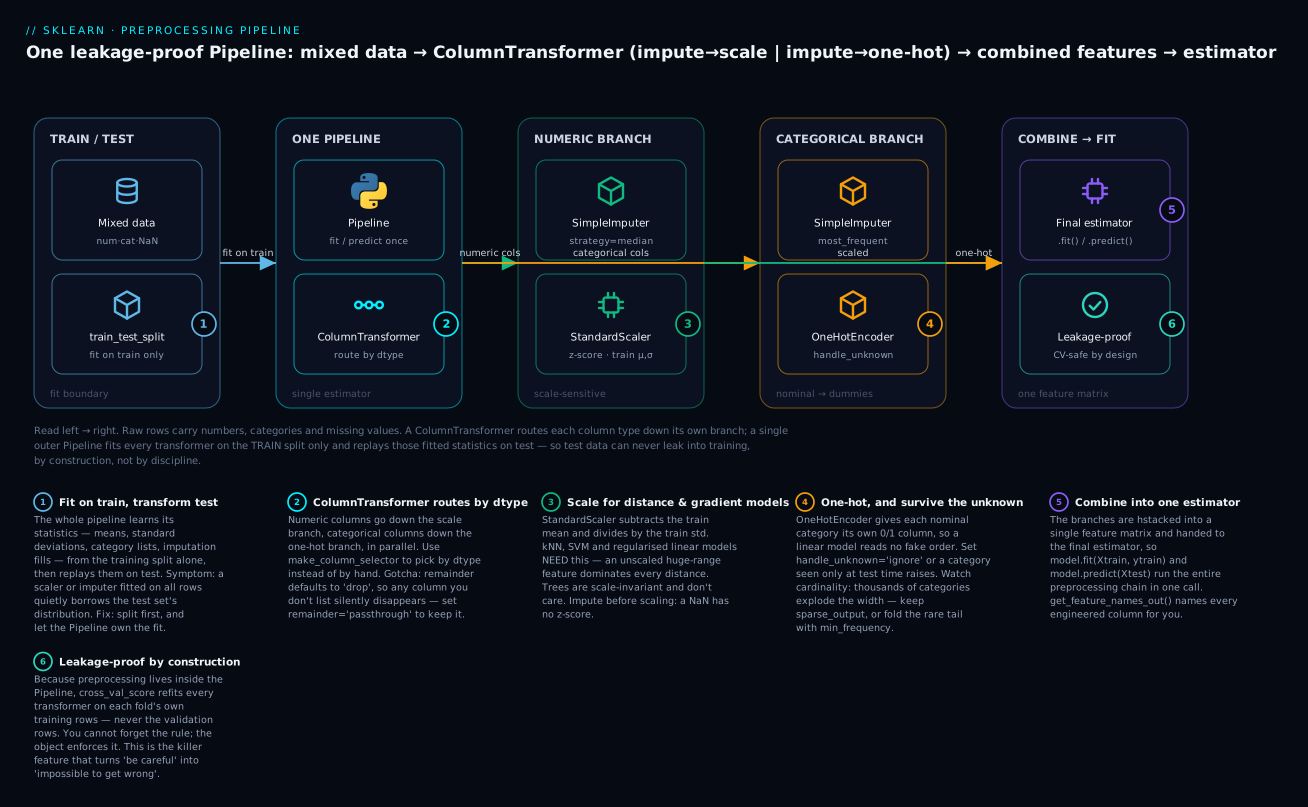
The six badges mark where beginners lose the most time. The fit-on-train boundary (1) is the rule the whole structure enforces. The ColumnTransformer routes by dtype (2) — and its remainder default silently drops any column you forget to list. The numeric branch scales (3) because kNN/SVM/regularised-linear need it and trees don’t. The categorical branch one-hots (4) with handle_unknown='ignore' so an unseen test category doesn’t crash. The branches combine into one estimator (5) so fit/predict is a single call. And the whole thing is leakage-proof (6) because preprocessing lives inside the Pipeline that cross-validation refits per fold.
Now build exactly that. Start from a realistic mixed dataset — customer churn, with numeric usage columns, categorical city/plan, and missing values sprinkled through both:
import pandas as pd
from sklearn.compose import ColumnTransformer, make_column_selector
from sklearn.impute import SimpleImputer

# X has: tenure_months, monthly_inr, logins_30d (numeric, some NaN)
#        city, plan (categorical, some None)
numeric     = ["tenure_months", "monthly_inr", "logins_30d"]
categorical = ["city", "plan"]

num_pipe = Pipeline([("impute", SimpleImputer(strategy="median")),
                     ("scale",  StandardScaler())])
cat_pipe = Pipeline([("impute", SimpleImputer(strategy="most_frequent")),
                     ("onehot", OneHotEncoder(handle_unknown="ignore"))])

pre = ColumnTransformer([("num", num_pipe, numeric),
                         ("cat", cat_pipe, categorical)])

model = Pipeline([("pre", pre), ("clf", LogisticRegression(max_iter=1000))])
model.fit(Xtr, ytr)                                   # ONE call does everything
print("test accuracy:", round(model.score(Xte, yte), 3))
print("features out:", list(model.named_steps["pre"].get_feature_names_out()))
test accuracy: 0.807
features out: ['num__tenure_months', 'num__monthly_inr', 'num__logins_30d',
 'cat__city_Bengaluru', 'cat__city_Chennai', 'cat__city_Delhi', 'cat__city_Mumbai',
 'cat__plan_enterprise', 'cat__plan_free', 'cat__plan_pro']
One fit call imputed missing numbers with the training median, scaled them, imputed missing categories with the training mode, one-hot-encoded them, stacked all ten resulting columns, and fitted the classifier — and score replayed every one of those transforms on the test set using the training statistics. The get_feature_names_out() even names each engineered column, prefixed by its branch (num__, cat__).
By default transformers return bare NumPy arrays, which lose your column names the moment they enter the pipeline — annoying when you want to inspect intermediate output. One global switch keeps DataFrames flowing all the way through:
from sklearn import set_config
set_config(transform_output="pandas")     # every transformer now returns a DataFrame
# StandardScaler().fit_transform(df) -> a DataFrame with named columns, not a bare ndarray
This makes debugging a ColumnTransformer far easier — you can .head() the output of any step and see labelled columns — at the cost of a little speed, so many teams switch it on in notebooks and off in production. Cross-validate the model and every fold is clean:
cv = cross_val_score(model, X, y, cv=5)
print(np.round(cv, 3), "mean", round(cv.mean(), 3))   # => [0.788 0.808 0.825 0.796 0.821] mean 0.807
Selecting columns by dtype, and the remainder trap
Listing columns by hand is tedious and drifts out of date. make_column_selector picks them by dtype instead:
pre_auto = ColumnTransformer([
    ("num", num_pipe, make_column_selector(dtype_include=np.number)),
    ("cat", cat_pipe, make_column_selector(dtype_include=object)),
])
# identical result: 0.807 — but the selector adapts if columns are added
Now the trap that catches everyone once. ColumnTransformer drops every column you don’t explicitly list. Its remainder parameter defaults to 'drop':
df3 = pd.DataFrame({"age": [25, 40, 33], "city": ["BLR", "DEL", "MUM"], "note": ["a", "b", "c"]})
ct = ColumnTransformer([("num", StandardScaler(), ["age"])])
print(ct.fit_transform(df3).shape)                            # => (3, 1)   city and note GONE
ct2 = ColumnTransformer([("num", StandardScaler(), ["age"])], remainder="passthrough")
print(ct2.fit_transform(df3).shape)                           # => (3, 3)   kept
The first transformer silently returned only the age column; city and note vanished with no warning. If your model mysteriously ignores half your features, check remainder. Use remainder='passthrough' to keep unlisted columns untouched, or remainder='drop' (the default) deliberately when you mean to discard them.
ColumnTransformer piece |
Purpose |
|---|---|
("name", transformer, columns) |
A named branch: apply transformer to columns |
columns as list of names |
Explicit selection (["city", "plan"]) |
make_column_selector(dtype_include=np.number) |
Select numeric columns automatically |
make_column_selector(dtype_include=object) |
Select text/categorical columns automatically |
remainder='drop' (default) |
Unlisted columns are discarded — the common surprise |
remainder='passthrough' |
Keep unlisted columns unchanged |
make_column_transformer(...) |
Terser constructor with auto-named branches |
.get_feature_names_out() |
Names of all output columns, branch-prefixed |
verbose_feature_names_out=False |
Drop the num__/cat__ prefixes if you find them noisy |
Both constructors have a terser “make” form that auto-names the parts — handy when you don’t need to reference steps by name:
| Verbose, explicit names | Terser, auto-named | What the shorthand does |
|---|---|---|
Pipeline([("sc", StandardScaler()), ("clf", LogisticRegression())]) |
make_pipeline(StandardScaler(), LogisticRegression()) |
Names steps from the lowercased class (standardscaler, logisticregression) |
ColumnTransformer([("num", T, cols)]) |
make_column_transformer((T, cols)) |
Auto-names each branch |
explicit ["tenure_months", "monthly_inr"] |
make_column_selector(dtype_include=np.number) |
Selects columns by dtype at fit time, so new columns are picked up |
Use the explicit form when you will tune nested parameters (clf__C) or inspect a step by name; use the make_ form for throwaway or obvious pipelines.
Feature engineering: helping the model see structure
Scaling and encoding make data usable; feature engineering makes it informative. The goal is to hand the model features that expose the structure you already know is there, so it doesn’t have to discover it from scratch.
PolynomialFeatures creates interactions and powers — turning [a, b] into [a, b, a², ab, b²] — which lets a linear model fit curves and cross-effects it otherwise couldn’t:
from sklearn.preprocessing import PolynomialFeatures
X = np.array([[2.0, 3.0], [4.0, 5.0]])
pf = PolynomialFeatures(degree=2, include_bias=False)
print(pf.fit_transform(X))                                  # => [[2 3 4 6 9] [4 5 16 20 25]]
print(list(pf.get_feature_names_out(["a", "b"])))           # => ['a', 'b', 'a^2', 'a b', 'b^2']

pf2 = PolynomialFeatures(degree=2, interaction_only=True, include_bias=False).fit(X)
print(list(pf2.get_feature_names_out(["a", "b"])))          # => ['a', 'b', 'a b']   no a^2, b^2
interaction_only=True keeps the cross-term ab but not the squares — useful when you suspect features interact but don’t want to model curvature. Beware degree: degree=3 on 100 features is hundreds of thousands of columns.
KBinsDiscretizer turns a continuous column into ordered bins — sometimes “young / middle / senior” is a better feature than a raw age, letting a linear model capture a non-linear age effect:
from sklearn.preprocessing import KBinsDiscretizer
ages = np.array([[19.0], [25.0], [34.0], [47.0], [63.0], [81.0]])
kb = KBinsDiscretizer(n_bins=3, encode="ordinal", strategy="quantile")
print(kb.fit_transform(ages).ravel())              # => [0. 0. 1. 1. 2. 2.]
print(np.round(kb.bin_edges_[0], 1))               # => [19.  29.5 55.  81. ]
Datetime features are almost always worth extracting by hand — a raw timestamp is nearly useless to a model, but day-of-week, hour, month, and is-weekend often carry real signal. A FunctionTransformer wraps any function so it slots into a Pipeline:
from sklearn.preprocessing import FunctionTransformer
def datetime_parts(col):
    dt = pd.to_datetime(col.iloc[:, 0])
    return pd.DataFrame({"dow": dt.dt.dayofweek, "hour": dt.dt.hour,
                         "month": dt.dt.month, "is_weekend": (dt.dt.dayofweek >= 5).astype(int)})
ft = FunctionTransformer(datetime_parts)
# "2026-07-04 23:30" -> dow=5, hour=23, month=7, is_weekend=1
| Transformer | Turns | Into | Use when |
|---|---|---|---|
PolynomialFeatures |
[a, b] |
[a, b, a², ab, b²] |
Linear model must fit curves/interactions |
KBinsDiscretizer |
continuous | ordinal bins / one-hot bins | A non-linear effect is better as buckets |
FunctionTransformer |
anything | your function’s output | Custom logic (datetime parts, logs) inside a Pipeline |
PowerTransformer |
skewed | more Gaussian | Heavy-tailed features hurt a linear/NN model |
SplineTransformer |
continuous | smooth basis functions | Flexible non-linearity without polynomial blow-up |
The two you will reach for most have a handful of parameters worth memorising:
| Transformer · parameter | Default | Effect |
|---|---|---|
PolynomialFeatures(degree=…) |
2 |
Highest power and interaction order generated |
PolynomialFeatures(include_bias=…) |
True |
True adds a constant 1 column; set False inside a Pipeline (the model has its own intercept) |
PolynomialFeatures(interaction_only=…) |
False |
True keeps a b, drops a², b² |
KBinsDiscretizer(n_bins=…) |
5 |
Number of bins per feature |
KBinsDiscretizer(encode=…) |
'onehot' |
'ordinal' → integer bins; 'onehot'/'onehot-dense' → dummies |
KBinsDiscretizer(strategy=…) |
'quantile' |
'uniform' equal-width · 'quantile' equal-count · 'kmeans' cluster-based |
The honest note that outranks all of these: domain knowledge beats brute force. A single feature you engineer because you understand the problem — “days since last login,” “price per square foot,” “is this transaction bigger than the customer’s usual” — routinely outperforms a mountain of automatic polynomial terms. PolynomialFeatures(degree=4) is not a substitute for understanding your data; it is what you try when you have run out of understanding. The best feature engineering is a conversation with someone who knows the business, not a bigger degree=.
Hands-on lab
You will build the full real-world pattern end to end: a mixed dataset, a ColumnTransformer inside a Pipeline, a one-call fit-and-score, then two demonstrations that make the leakage and encoding lessons concrete. Everything runs on the venv from the top of the lesson (scikit-learn, numpy, pandas installed). Create churn.py and build it up step by step; every output below is exact.
Step 1 — Build a realistic mixed dataset.
import numpy as np
import pandas as pd
from sklearn.model_selection import train_test_split, cross_val_score
from sklearn.compose import ColumnTransformer, make_column_selector
from sklearn.pipeline import Pipeline
from sklearn.preprocessing import StandardScaler, OneHotEncoder, OrdinalEncoder
from sklearn.impute import SimpleImputer
from sklearn.linear_model import LogisticRegression, LinearRegression
from sklearn.feature_selection import SelectKBest, f_classif

def make_customers(n=1200, seed=0):
    rng = np.random.default_rng(seed)
    city = rng.choice(["Bengaluru", "Delhi", "Mumbai", "Chennai"], size=n)
    plan = rng.choice(["free", "pro", "enterprise"], size=n, p=[0.6, 0.3, 0.1])
    tenure = rng.gamma(2.0, 12.0, size=n).round(1)
    monthly = rng.normal(800, 300, size=n).clip(50).round(2)
    logins = rng.poisson(20, size=n).astype(float)
    signal = (0.9 * (plan == "free") - 0.03 * tenure - 0.04 * logins
              + 0.0005 * monthly + rng.normal(0, 0.5, size=n))
    churn = (signal > np.quantile(signal, 0.7)).astype(int)
    df = pd.DataFrame({"city": city, "plan": plan, "tenure_months": tenure,
                       "monthly_inr": monthly, "logins_30d": logins, "churn": churn})
    df.loc[rng.choice(n, 80, replace=False), "tenure_months"] = np.nan   # holes
    df.loc[rng.choice(n, 60, replace=False), "city"] = None
    return df

df = make_customers()
print(df.head(4).to_string(index=False))
print("\nmissing per column:\n" + df.isna().sum().to_string())
X, y = df.drop(columns="churn"), df["churn"]
Xtr, Xte, ytr, yte = train_test_split(X, y, test_size=0.25, random_state=0, stratify=y)
print(f"\ntrain {Xtr.shape}  test {Xte.shape}  churn rate {y.mean():.2f}")
   city plan  tenure_months  monthly_inr  logins_30d  churn
Chennai free            6.0       584.25        27.0      0
 Mumbai  pro           16.7      1110.39        17.0      0
 Mumbai  pro           16.5      1122.58        13.0      0
  Delhi  pro            6.0      1395.84        15.0      0

missing per column:
city             60
plan              0
tenure_months    80
monthly_inr       0
logins_30d        0
churn             0

train (900, 5)  test (300, 5)  churn rate 0.30
What just happened: a mixed dataset — two text columns, three numeric, 60 missing cities and 80 missing tenures — and a stratified split so train and test share the 30% churn rate. This is the shape of every real tabular problem.
Step 2 — One ColumnTransformer + Pipeline, fit and score in one call.
numeric     = ["tenure_months", "monthly_inr", "logins_30d"]
categorical = ["city", "plan"]
num_pipe = Pipeline([("impute", SimpleImputer(strategy="median")),
                     ("scale",  StandardScaler())])
cat_pipe = Pipeline([("impute", SimpleImputer(strategy="most_frequent")),
                     ("onehot", OneHotEncoder(handle_unknown="ignore"))])
pre = ColumnTransformer([("num", num_pipe, numeric),
                         ("cat", cat_pipe, categorical)])
model = Pipeline([("pre", pre), ("clf", LogisticRegression(max_iter=1000))])

model.fit(Xtr, ytr)                                # impute+scale+encode+fit, one call
print("test accuracy      :", round(model.score(Xte, yte), 3))
print("engineered features:", model.named_steps["pre"].get_feature_names_out().shape[0])
test accuracy      : 0.807
engineered features: 10
What just happened: one fit handled missing values, scaling, and encoding for five raw columns, produced ten engineered features, and trained a classifier — and score replayed every transform on the test set with the training statistics. No leakage was possible, because you never touched the test set with a fit.
Step 3 — Prove the pipeline is cross-validation-safe.
cv = cross_val_score(model, X, y, cv=5)
print("folds:", np.round(cv, 3), " mean:", round(cv.mean(), 3))
folds: [0.788 0.808 0.825 0.796 0.821] mean: 0.807
What just happened: cross_val_score refit the entire pipeline — imputers, scaler, encoder, classifier — five times, each on a different four-fifths of the data, and scored on the held-out fifth. Every fold’s preprocessing learned only from that fold’s training rows. This is what an honest score looks like.
Step 4a — See scaler leakage as a mechanism.
xtr = Xtr[["monthly_inr"]].to_numpy()
xte = Xte[["monthly_inr"]].to_numpy()[:4]
all_test = Xte[["monthly_inr"]].to_numpy()
fit_train = StandardScaler().fit(xtr)
fit_all   = StandardScaler().fit(np.vstack([xtr, all_test]))
print("scaled on TRAIN only:", fit_train.transform(xte).ravel().round(4))
print("scaled on ALL data  :", fit_all.transform(xte).ravel().round(4))
scaled on TRAIN only: [ 0.0348 -1.2421 -0.2303 -0.2518]
scaled on ALL data  : [ 0.0274 -1.2349 -0.2347 -0.2559]
What just happened: the same four test rows got different scaled values depending on whether the scaler was allowed to see the test set during fit. The difference is small — for a plain scaler it usually is — but it is real leakage: test information changed the training inputs. The point of the next step is that the same mistake is not always small.
Step 4b — See the same mistake turn deadly.
rng = np.random.default_rng(1)
Xn = rng.normal(size=(100, 5000))       # pure noise features
yn = rng.integers(0, 2, size=100)       # target independent of X -> truth = 0.5
picked = SelectKBest(f_classif, k=20).fit(Xn, yn)         # peeks at ALL labels
leaky  = cross_val_score(LogisticRegression(max_iter=1000), picked.transform(Xn), yn, cv=5).mean()
safe   = Pipeline([("sel", SelectKBest(f_classif, k=20)),
                   ("clf", LogisticRegression(max_iter=1000))])
honest = cross_val_score(safe, Xn, yn, cv=5).mean()
print(f"select-then-CV (leaky): {leaky:.3f}   Pipeline (honest): {honest:.3f}   truth ~0.500")
select-then-CV (leaky): 0.910 Pipeline (honest): 0.470 truth ~0.500
What just happened: selecting features on the full dataset before cross-validating fabricated 91% accuracy from pure noise — the selector cherry-picked features that correlated with the labels by chance, using rows it would later be “tested” on. The Pipeline, selecting inside each fold, reported the honest ~0.47. If you take one number from this lesson, take the gap between 0.910 and 0.500.
Step 5 — OrdinalEncoder poisons a linear model; OneHot fixes it.
from sklearn.tree import DecisionTreeRegressor
from sklearn.metrics import r2_score
rng = np.random.default_rng(0)
cities = np.array(["Bengaluru", "Chennai", "Delhi", "Mumbai"])
eff = {"Bengaluru": 30.0, "Chennai": 90.0, "Delhi": 45.0, "Mumbai": 80.0}   # non-monotonic
cc = rng.choice(cities, size=2000)
price = np.array([eff[c] for c in cc]) + rng.normal(0, 5, size=2000)
Xc = cc.reshape(-1, 1)
Xc_tr, Xc_te, yc_tr, yc_te = train_test_split(Xc, price, test_size=0.3, random_state=0)
oe  = OrdinalEncoder().fit(Xc_tr)
ohe = OneHotEncoder(sparse_output=False, handle_unknown="ignore").fit(Xc_tr)
lin_o  = LinearRegression().fit(oe.transform(Xc_tr), yc_tr)
lin_h  = LinearRegression().fit(ohe.transform(Xc_tr), yc_tr)
tree_o = DecisionTreeRegressor(random_state=0).fit(oe.transform(Xc_tr), yc_tr)
print("Linear + Ordinal  R2 =", round(r2_score(yc_te, lin_o.predict(oe.transform(Xc_te))), 3))
print("Linear + OneHot   R2 =", round(r2_score(yc_te, lin_h.predict(ohe.transform(Xc_te))), 3))
print("Tree   + Ordinal  R2 =", round(r2_score(yc_te, tree_o.predict(oe.transform(Xc_te))), 3))
Linear + Ordinal  R2 = 0.201   <- poisoned
Linear + OneHot   R2 = 0.957   <- fixed
Tree   + Ordinal  R2 = 0.957   <- tree copes
What just happened: forcing a fake order (Bengaluru=0 … Mumbai=3) onto nominal cities crippled the linear model to R²=0.20, because it could only fit a single slope through arbitrary codes. One-hot encoding — a column per city — let it fit each city’s effect independently and hit R²=0.96. The tree survived the ordinal codes because it can split the integer axis repeatedly. Encoding is a modelling decision, not a formatting chore.
You now have the full pattern: a mixed dataset turned into a clean matrix by a ColumnTransformer, wrapped in a Pipeline that fits on train only, scores in one call, cross-validates without leakage, and encodes categoricals in the way each model actually needs.
Common mistakes and troubleshooting
| Symptom / traceback | Cause | Fix |
|---|---|---|
| Great CV score, terrible production score | Preprocessing fitted on all data before the split — leakage | Put every transformer in a Pipeline; let cross_val_score refit per fold |
ValueError: Found unknown categories ['X'] in column 0 during transform |
A category appeared at test/predict time that wasn’t in fit |
OneHotEncoder(handle_unknown='ignore') (or OrdinalEncoder(handle_unknown='use_encoded_value', unknown_value=-1)) |
ValueError: Input X contains NaN |
Model or scaler received missing values | Add a SimpleImputer before the scaler in the numeric branch |
| kNN/SVM accuracy near random despite good features | Forgot to scale — a huge-range feature dominates the distance | StandardScaler (or RobustScaler) before the model |
| Linear model far worse than a tree on categorical data | OrdinalEncoder on nominal columns injected a fake order |
OneHotEncoder for nominal; ordinal only for truly ordered categories |
| Half your columns seem ignored by the model | ColumnTransformer remainder='drop' silently dropped unlisted columns |
List every column, use make_column_selector, or remainder='passthrough' |
ValueError: Invalid parameter 'clff' for estimator Pipeline(...) |
Typo in a Pipeline step name when setting params | Match the step name exactly; check pipe.get_params().keys() |
NotFittedError: This StandardScaler instance is not fitted yet |
Called transform/get_feature_names_out before fit |
fit (or fit_transform) first; inside a Pipeline this is automatic |
MemoryError / process killed after one-hot |
One-hot on a high-cardinality column exploded to millions of columns | Keep sparse_output=True; use min_frequency/max_categories; or TargetEncoder |
ValueError: X has 7 features, but ... is expecting 8 features |
Transformed data has a different column count than at fit |
Feed the same columns in the same order — another reason to use a Pipeline |
| Test set scaled differently than train | Called fit_transform on test (refits!) instead of transform |
transform on test, fit_transform on train only — or let the Pipeline do it |
| Model can’t accept the encoder’s output | OneHotEncoder returned a sparse matrix; the estimator wants dense |
sparse_output=False, or use a pipeline step that accepts sparse |
dropped category and unknown look identical |
drop='first' + handle_unknown='ignore' — both encode all-zeros |
Don’t combine them; use drop='if_binary', or skip drop |
Three of these deserve extra words because they cost the most hours.
1. Leakage is silent, and small leaks lull you into big ones. Nothing raises when you fit_transform the whole dataset before splitting. The score just comes out too high, and because a scaler’s leak is often tiny, you conclude the practice is harmless — right up until the day you add a TargetEncoder or a SelectKBest and ship a model that tested at 0.91 and performs at 0.50. The only durable defence is structural: never fit a transformer outside a Pipeline, and always evaluate with cross_val_score/GridSearchCV wrapping the whole Pipeline. Then the mistake is not “usually small” — it is impossible.
2. The remainder drop is the quiet feature-eater. ColumnTransformer discards any column you don’t name, with no warning. A model that mysteriously underperforms, or a get_feature_names_out() that is shorter than you expected, is almost always this. Print the output shape after your ColumnTransformer and confirm it has the columns you think it does; reach for make_column_selector so new columns are picked up automatically, or set remainder='passthrough' when you mean to keep the rest.
3. handle_unknown is not optional in production. In a notebook, every category is in your data, so the default handle_unknown='error' never fires. Then you deploy, a customer from a city that wasn’t in the training set arrives, and transform throws ValueError: Found unknown categories — an outage caused by a value you never saw. Set handle_unknown='ignore' on every OneHotEncoder that will ever touch live data, and unknown_value=-1 on every OrdinalEncoder. Decide what “unseen category” means before it happens, not during the incident.
Cheat-sheet
| Task | Code |
|---|---|
| Standardise (z-score) | StandardScaler() → mean 0, std 1 |
Scale to [0,1] |
MinMaxScaler() |
| Scale robustly (outliers) | RobustScaler() → median & IQR |
| Unit-length rows | Normalizer() (per-sample, not per-column) |
| One-hot a nominal column | OneHotEncoder(handle_unknown='ignore') |
| One-hot for a linear model | OneHotEncoder(drop='if_binary') |
| Dense one-hot output | OneHotEncoder(sparse_output=False) |
| Encode an ordered column | OrdinalEncoder(categories=[['low','med','high']]) |
| Tame high cardinality | OneHotEncoder(min_frequency=…, max_categories=…) or TargetEncoder() |
| Fill numeric holes | SimpleImputer(strategy='median') |
| Fill categorical holes | SimpleImputer(strategy='most_frequent') |
| Smart imputation | KNNImputer(n_neighbors=5) |
| Flag imputed values | SimpleImputer(add_indicator=True) |
| Chain transformers + model | Pipeline([('pre', pre), ('clf', model)]) |
| Auto-named pipeline | make_pipeline(StandardScaler(), LogisticRegression()) |
| Per-column-type preprocessing | ColumnTransformer([('num', num_pipe, numeric), ('cat', cat_pipe, cat)]) |
| Select columns by dtype | make_column_selector(dtype_include=np.number) |
| Keep unlisted columns | ColumnTransformer(..., remainder='passthrough') |
| Fit everything, once | model.fit(X_train, y_train) |
| Score without leakage | model.score(X_test, y_test) |
| Honest cross-validation | cross_val_score(model, X, y, cv=5) |
| Interactions & powers | PolynomialFeatures(degree=2, include_bias=False) |
| Bin a continuous column | KBinsDiscretizer(n_bins=4, encode='ordinal') |
| Custom transform in a pipeline | FunctionTransformer(my_func) |
| Name the engineered columns | pre.get_feature_names_out() |
| Tune a nested param | pipe.set_params(clf__C=10) |
| DataFrame output from transformers | from sklearn import set_config; set_config(transform_output='pandas') |
| The rule | fit on train only; transform on test — or use a Pipeline so you can’t do otherwise |
Interview and exam questions
Q: What is the difference between a transformer and a predictor in scikit-learn, and what methods define each?
A: Both are estimators and both learn via fit. A transformer changes the data and has fit, transform, and fit_transform (StandardScaler, OneHotEncoder, SimpleImputer). A predictor makes predictions and has fit and predict (LogisticRegression, RandomForestClassifier). The uniformity is the whole point: because every object shares this interface, you can compose them freely into a Pipeline, which is itself an estimator. Learned state always ends in a trailing underscore (mean_, categories_), and fit always returns self.
Q: Why do some models need feature scaling and others don’t? Give an example of each. A: Models that measure distance (kNN, SVM/RBF, K-Means) or sum weighted features with a size-based penalty (regularised linear models, neural nets) need scaling, because a large-range feature dominates the distance or the penalty. In a demonstration with an informative small-scale feature next to a pure-noise huge-scale feature, kNN scored 0.53 raw and 0.86 scaled. Tree-based models (decision tree, random forest, gradient boosting) do not need scaling: they split on per-feature thresholds, and the answer to “is x > 5?” is unchanged by rescaling x — a random forest scored 0.864 both raw and scaled. Scaling a tree is harmless but pointless.
Q: When would you use StandardScaler vs MinMaxScaler vs RobustScaler?
A: StandardScaler (subtract mean, divide by std → mean 0, std 1) is the sensible default for roughly-symmetric data. MinMaxScaler (map min/max to [0,1]) when you need a bounded range and have no outliers — a single outlier squashes all real data into a sliver, because the outlier owns the max. RobustScaler (subtract median, divide by IQR) when outliers are present and can’t be removed — it centres on the median and scales by the interquartile range, both barely moved by extremes. In one test, a column [10,12,11,13,9,1000] left StandardScaler with a “typical” mean of 175.8 (near none of the data), while RobustScaler’s center was 11.5 (the real middle).
Q: Explain the difference between OneHotEncoder and OrdinalEncoder and the trap with OrdinalEncoder.
A: OneHotEncoder gives each category its own 0/1 column, implying no order — correct for nominal data. OrdinalEncoder assigns integers 0,1,2,… — correct only when a real order exists (S<M<L). The trap: ordinal-encoding a nominal column (e.g. cities → 0,1,2,3) injects a fake order, and a linear model believes it, fitting a single slope through arbitrary codes. Measured on non-monotonic city effects, a linear model scored R²=0.20 with ordinal encoding and R²=0.96 with one-hot. Trees are largely immune (they split the integer axis repeatedly), so the poison is specifically ordinal-nominal-into-a-linear-model.
Q: What is handle_unknown='ignore', and why does it matter in production?
A: By default, if OneHotEncoder.transform meets a category that wasn’t present during fit, it raises ValueError: Found unknown categories. In a notebook this never fires because all categories are in your data; in production, a new city/product/value arrives and crashes the service. handle_unknown='ignore' instead encodes the unseen category as all-zeros, so the model degrades gracefully instead of erroring. It should be set on essentially every encoder that will touch live data.
Q: Why must you fit transformers on the training set only? Describe a concrete failure. A: Because a transformer learns parameters from data (a mean, an IQR, a category list, a fill value), and if it learns them from data the model shouldn’t see, that information leaks and inflates your score. Concrete failure: selecting the 20 features most correlated with the target on the whole dataset — including future validation rows — before cross-validating, on a target that is pure noise, produced 91% accuracy where the truth is 50%. Fitting the selection inside each fold (via a Pipeline) correctly reported ~47%. Plain scaler leakage is usually small, but you can’t safely reason case by case about which steps are dangerous, so you make leakage structurally impossible.
Q: How does a Pipeline prevent data leakage, and why is that better than being careful?
A: A Pipeline is an estimator whose fit runs each step’s fit_transform on the training data and whose predict/score runs each step’s transform only — it never calls fit on the test data. Crucially, when you pass a Pipeline to cross_val_score or GridSearchCV, the entire chain is refit on each fold’s training portion, so every fold’s preprocessing learns only from that fold’s training rows. That converts “remember to fit on train only, on every fold, forever” into a structural guarantee you cannot violate. Discipline fails eventually; structure doesn’t.
Q: What does ColumnTransformer do, and what is the remainder gotcha?
A: ColumnTransformer applies different transformers to different column subsets — e.g. StandardScaler on numeric columns and OneHotEncoder on categorical — and horizontally stacks the results into one matrix. The gotcha: remainder defaults to 'drop', so any column you don’t explicitly list is silently discarded with no warning. Symptoms are a model that ignores features or a shorter-than-expected get_feature_names_out(). Fix with remainder='passthrough' to keep unlisted columns, or make_column_selector to pick columns by dtype so nothing is forgotten.
Q: How would you handle a categorical feature with 10,000 unique values?
A: Not with plain one-hot — that produces 10,000 columns (in one test, 20,000 pincode rows made a 98-million-cell matrix, 99.98% zeros). Options: keep sparse_output=True so only the non-zeros are stored; fold the rare tail with min_frequency/max_categories (which collapsed 496 columns to 6 in a demo); or switch encoding entirely to target encoding (TargetEncoder, replace each category with its mean target) or hashing (category_encoders.HashingEncoder), both fixed-width regardless of cardinality. Target encoding uses the label, so it must run inside CV folds to avoid leakage.
Q (coding): Write a leakage-free pipeline that scales numeric columns, one-hot-encodes categoricals, imputes both, and fits a classifier — and cross-validate it. A:
num = make_column_selector(dtype_include=np.number)
cat = make_column_selector(dtype_include=object)
pre = ColumnTransformer([
    ("num", Pipeline([("imp", SimpleImputer(strategy="median")),
                      ("sc",  StandardScaler())]), num),
    ("cat", Pipeline([("imp", SimpleImputer(strategy="most_frequent")),
                      ("oh",  OneHotEncoder(handle_unknown="ignore"))]), cat),
])
model = Pipeline([("pre", pre), ("clf", LogisticRegression(max_iter=1000))])
scores = cross_val_score(model, X, y, cv=5)   # every fold refits pre on its own train rows
Because preprocessing lives inside the Pipeline, cross_val_score refits it per fold and no test data leaks — this is the canonical production pattern.
Q: What does fit_transform do, and when must you never call it?
A: fit_transform(X) is fit(X) followed by transform(X), sometimes fused for speed, with a guaranteed-identical result. Call it on your training set. Never call it on your test/validation set: doing so refits the transformer on the test data, learning test statistics and leaking. On test you call plain transform. Inside a Pipeline this is handled for you — the Pipeline calls fit_transform on train during fit and transform on test during predict.
Key takeaways
- Every scikit-learn object is an estimator with one uniform interface. Transformers have
fit/transform/fit_transform; predictors havefit/predict. Learned state ends in a trailing underscore (mean_,categories_), andfitreturnsself. That consistency is what lets you compose everything into a Pipeline — learn the interface once, drive the whole library. - Scale for distance-based and gradient/regularised models; don’t bother for trees. kNN and SVM collapse to near-random on unscaled data (0.53 → 0.86 in the demo) because a large-range feature owns the distance metric; regularised linear models and neural nets converge faster and penalise fairly when scaled (132 → 9 iterations). Trees are scale-invariant. Use
StandardScalerby default,RobustScalerwhen outliers are present,MinMaxScaleronly when you need a bounded range and have no outliers. - Encode with the model in mind.
OneHotEncoderfor nominal categories — each gets its own column, no fake order.OrdinalEncoderonly for genuinely ordered categories. Ordinal-encoding nominal data into a linear model is poison: R²=0.20 vs 0.96 for one-hot on the same data. Always sethandle_unknown='ignore'for production, and defend against high cardinality withmin_frequency, sparse output, or target encoding. - Impute before you scale or encode, and learn the fill from train only.
SimpleImputer('median')for skewed numerics,'most_frequent'for categoricals,KNNImputerwhen features are correlated. A model given aNaNrefuses to fit; a fill learned from the test set leaks. - The one rule that governs everything: fit on train, transform test. Leakage — fitting any transformer on data the model shouldn’t see — produces scores that look great and evaporate in production. A plain scaler leaks little, but the same mistake with feature selection fabricated 91% accuracy from pure noise. You cannot safely reason step-by-step about what’s dangerous, so you make leakage impossible instead of unlikely.
Pipelinemakes leakage impossible by construction — this is the centrepiece. It chains transformers and a model into one estimator that never fits on test data, andcross_val_score/GridSearchCVrefit the whole chain on each fold’s training rows. Discipline fails; structure doesn’t. Every real model should be a Pipeline.ColumnTransformeris the real-world pattern: different preprocessing per column type. Scale numerics, one-hot categoricals, impute both, recombine into one matrix — all inside the outer Pipeline. Usemake_column_selectorto pick by dtype, and watchremainder, which silently drops every column you forget to list.- Feature engineering beats brute force when it comes from understanding.
PolynomialFeatures,KBinsDiscretizer, and datetime extraction expose structure a model would otherwise have to discover — but a single feature built from domain knowledge routinely outperforms a mountain of automatic polynomial terms.degree=4is what you try when you’ve run out of understanding, not a substitute for it.
This is Part 1 of the scikit-learn arc. You can now turn any messy spreadsheet into a clean, leakage-proof feature matrix and wrap it in a Pipeline that behaves like a single model. Part 2 takes that Pipeline and swaps in the algorithms — logistic regression, trees, forests, gradient boosting, SVMs — and teaches how each learns and when to reach for it. Part 3 puts the whole Pipeline inside cross-validation and hyperparameter search, so you tune the preprocessing and the model together, honestly, without ever leaking a single test row. The habit you built here — everything inside one Pipeline, fit on train only — is the foundation both of those parts stand on. For the data-wrangling that feeds this stage, revisit pandas groupby, merge and missing data and NumPy arrays, broadcasting and vectorization; for the concepts underneath the models, ML fundamentals: supervised vs unsupervised; and for the class-design instincts behind the estimator API, designing domain models with dataclasses.