There is a moment, early in everyone’s machine-learning life, that feels like triumph and is actually the trap. You train a model, you call .score(), and it prints 1.0. Perfect. Flawless. You ship it — or you would, if you didn’t already sense something is wrong. It is wrong. A model that scores 100% on the data it was trained on has, in the worst case, learned nothing except how to look up the answers it was handed. Show it one new row and it may be worse than a coin flip.
This lesson is about the rigor that separates real machine learning from copy-paste: how to split data so a score means something, how to catch the data leakage that silently inflates results until the day they collapse in production, and how to choose an evaluation metric that reflects what you actually care about — because on the imbalanced datasets you meet in the real world (fraud, disease, churn, defects), the most popular metric of all, accuracy, will look magnificent while your model catches almost nothing.
Everything below was executed on Python 3.12.3 with scikit-learn 1.9.0 (plus NumPy 2.5.1, pandas 3.0.3, and matplotlib 3.11.0); every number, confusion matrix, and traceback is copied from those runs, not paraphrased. You need one install, in a virtual environment:
python3 -m venv .venv
source .venv/bin/activate          # Windows: .venv\Scripts\activate
python -m pip install scikit-learn numpy pandas matplotlib
This lesson is the evaluation half of the ML story. It assumes you know what a model is — the ML fundamentals lesson covers supervised vs unsupervised learning and the fit/predict shape — and it leans on tools from earlier: NumPy arrays for the numbers, pandas group-and-merge for the data wrangling, and matplotlib for the ROC and precision-recall curves you’ll plot near the end. Where this lesson quotes a p-value or an R², the course’s statistics lesson on hypothesis testing and regression develops the underlying theory; here we stay hands-on and empirical.
Why this matters
A machine-learning model is a function fitted to examples. You give it inputs X and known answers y, and it adjusts itself until its predictions on those examples are good. The whole enterprise rests on one assumption: that being good on the examples you have transfers to being good on the examples you don’t — tomorrow’s transactions, next week’s patients, the rows you haven’t seen. That transfer is called generalization, and it is the only thing that matters. A model that cannot generalize is a very expensive lookup table.
The problem is that a model can become good at the training examples in two completely different ways, and from the inside they look identical. It can learn the real pattern — the genuine relationship between inputs and outputs that will hold on new data. Or it can memorize — carve out an elaborate rule for each training row that nails those specific answers and captures no transferable pattern at all. Both produce a beautiful training score. Only one produces a useful model. This is the tension at the heart of the field: overfitting (memorizing noise as if it were signal) versus underfitting (too simple to capture the real pattern), and the entire practice of evaluation exists to tell them apart.
You cannot tell them apart by looking at the training score, because memorization maximizes it. The only way to measure generalization is to hold back data the model never saw during training and score it on that. That single idea — judge the model on data it did not learn from — is the foundation everything in this lesson is built on. Get it right and your numbers become trustworthy. Get it wrong — evaluate on training data, let test information leak into training, or pick a metric blind to your class imbalance — and you will ship models that shine in the notebook and fail in the world, which is the single most common way machine-learning projects die.
The stakes are highest exactly where the data is imbalanced, which is most places worth modeling. Fraud is rare. Disease is rare. The defective part, the churning customer, the click that converts — all rare. And when one class is rare, the metric everyone reaches for first, accuracy, becomes actively misleading: a fraud detector that flags nothing is 98% accurate on data that is 2% fraud, and 98% sounds like success. This lesson will make that failure concrete, on a real dataset, and then hand you the metrics that see through it.
A model that memorizes: overfitting in twelve lines
Let’s make the trap fail in front of us before we fix it. We’ll use the Wisconsin breast-cancer dataset that ships with scikit-learn (569 samples, 30 numeric features, a benign/malignant label), split it into a part to train on and a part to judge on, and fit a decision tree — a model that, left unconstrained, will keep splitting the data into ever-smaller boxes until each training point sits in its own box. That is memorization made mechanical.
from sklearn.datasets import load_breast_cancer
from sklearn.model_selection import train_test_split
from sklearn.tree import DecisionTreeClassifier

X, y = load_breast_cancer(return_X_y=True)
Xtr, Xte, ytr, yte = train_test_split(X, y, test_size=0.25,
                                      stratify=y, random_state=42)

full = DecisionTreeClassifier(random_state=42)          # no depth limit
full.fit(Xtr, ytr)
print(f"full tree    depth={full.get_depth()}  "
      f"train={full.score(Xtr, ytr):.3f}  test={full.score(Xte, yte):.3f}")

pruned = DecisionTreeClassifier(max_depth=3, random_state=42)
pruned.fit(Xtr, ytr)
print(f"depth-3 tree depth={pruned.get_depth()}  "
      f"train={pruned.score(Xtr, ytr):.3f}  test={pruned.score(Xte, yte):.3f}")
full tree    depth=7  train=1.000  test=0.923
depth-3 tree depth=3  train=0.977  test=0.944
Read those two lines slowly, because they contain the whole lesson in miniature.
| Model | Train score | Test score | Train − test gap | Verdict |
|---|---|---|---|---|
| Full tree (unlimited depth) | 1.000 | 0.923 | 0.077 | Overfit — memorized the training set |
| Depth-3 tree (constrained) | 0.977 | 0.944 | 0.033 | Healthier — and better on new data |
The unconstrained tree achieved a perfect training score. Every single training patient classified correctly. If the training score were your evidence, you would ship the full tree and call the simpler one worse. But on the held-out quarter of the data — the patients neither model was trained on — the full tree scores 0.923 while the deliberately handicapped depth-3 tree scores 0.944. The simpler model generalizes better. The extra depth the full tree used didn’t learn more signal; it learned the noise particular to those 426 training rows, and that noise doesn’t repeat in the test set. That gap between a perfect training score and a mediocre test score is the fingerprint of overfitting, and it is invisible unless you hold data back.
This is why the first and most important thing you do to a dataset is split it.
Three sets, three jobs: train, validation, test
The clean discipline uses not two piles of data but three, each with a single, non-overlapping job. Confusing them is one of the most common mistakes in applied ML, so let’s be precise about what each is for.
| Set | Typical size | The model uses it to… | You use it to… | Touched how often |
|---|---|---|---|---|
| Training | 60–80% | Fit its parameters (learn) | — | Constantly |
| Validation | 10–20% | — | Tune: pick models, hyperparameters, threshold | Repeatedly, during development |
| Test | 10–20% | — | Estimate real-world performance, once | Exactly once, at the very end |
The training set is what the model learns from — it sees these inputs and answers and adjusts itself. The validation set is how you make decisions during development: is a random forest better than logistic regression here, should max_depth be 3 or 8, where should I put the decision threshold? You try something, score it on validation, keep what wins. The test set is the final exam. It exists to answer one question — how will this model do on data it has never influenced in any way? — and it can only answer that question honestly if it stays sealed until every other decision is locked.
Which brings us to the rule that this entire lesson orbits, the one professional ML people will repeat until it sounds like a mantra:
The golden rule: never touch the test set until the very end. Not to pick a model. Not to tune a threshold. Not to “just check.” The moment a decision is influenced by the test score, the test set has quietly become part of training, and its estimate of new-data performance is corrupted — optimistically, invisibly, and permanently.
The reason is subtle and worth internalizing. Every time you look at a score and make a choice to improve it, you are fitting something to that data — if not the model’s parameters, then your own decisions. Do that against the validation set and it’s fine; that’s the validation set’s job, and it’s why we don’t report validation scores as the final word either. But do it against the test set and you’ve spent the one clean estimate you had. A test set you tuned against is no longer a test set. This is the actual mechanism behind “it worked in the notebook and failed in production”: the notebook number had been contaminated by dozens of small peeks, each one nudging the choice toward what happened to work on those particular held-out rows.
Here is the whole discipline as one left-to-right pipeline — data splits first, the test set is sealed, all selection happens with cross-validation on the training portion, and the test set is unsealed exactly once for the final number. The red node marks the leakage trap we’ll dissect next.
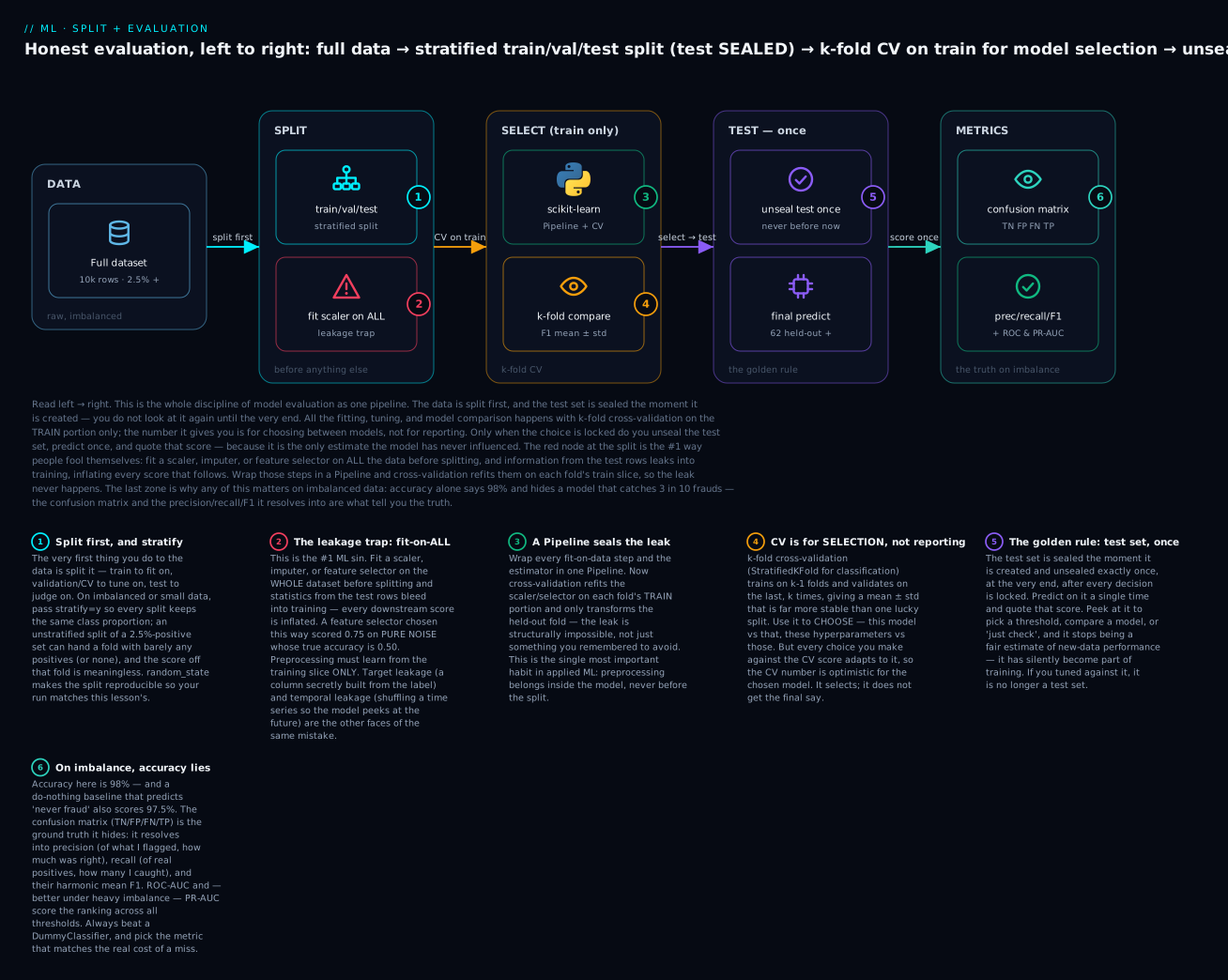
A practical note on how the three sets show up in code. You rarely make three explicit slices by hand. Instead you split once into train-plus-validation and test, seal the test set, and then get your validation signal from cross-validation on the train-plus-validation part — which reuses the same data as validation many times over, and which the middle sections of this lesson are devoted to. So in practice: train_test_split to carve off the sealed test set, then cross_val_score on what remains to make every development decision. Three jobs, two lines.
train_test_split in practice
train_test_split from sklearn.model_selection is the workhorse. It shuffles the rows and slices them into a train part and a test part. Its defaults are mostly sensible and its three most important arguments each prevent a specific, common mistake.
| Argument | Default | What it does | Why you set it |
|---|---|---|---|
test_size |
0.25 |
Fraction (or count) held out for testing | Balance: more test = steadier score, less train = weaker model |
train_size |
rest | Fraction for training | Usually left implicit as 1 − test_size |
random_state |
None |
Seed for the shuffle | Reproducibility — same seed, same split, every run |
stratify |
None |
Column to preserve class proportions on | Imbalance safety — keeps each split’s class balance equal to the whole |
shuffle |
True |
Shuffle before splitting | Turn off for time series (see leakage) |
random_state makes the split reproducible. Without it, every run reshuffles and you get a different train/test partition — so your scores wobble run to run and you can never tell whether a change helped or you just got a luckier split. Pin it (any integer) and the split is deterministic:
import numpy as np
from sklearn.datasets import make_classification
from sklearn.model_selection import train_test_split

X, y = make_classification(n_samples=300, n_features=10, n_informative=4,
                           weights=[0.90], class_sep=1.0, random_state=7)

# same seed -> byte-for-byte identical test set
_, Xte_a, _, _ = train_test_split(X, y, test_size=0.25, random_state=0)
_, Xte_b, _, _ = train_test_split(X, y, test_size=0.25, random_state=0)
_, Xte_c, _, _ = train_test_split(X, y, test_size=0.25, random_state=99)
print("seed 0 twice  -> identical:", np.array_equal(Xte_a, Xte_b))
print("seed 0 vs 99  -> identical:", np.array_equal(Xte_a, Xte_c))
seed 0 twice  -> identical: True
seed 0 vs 99  -> identical: False
stratify=y protects you on imbalanced data. A plain random split can, by chance, deal an unrepresentative hand — too few positives in the test set, or too few in the training set. On a 300-row dataset that is only ~10% positive, watch how the count of positives in the test set swings across random seeds when you don’t stratify, and how it stays pinned when you do:
for s in range(8):
    *_, y_plain = train_test_split(X, y, test_size=0.25, random_state=s)
    *_, y_strat = train_test_split(X, y, test_size=0.25, stratify=y, random_state=s)
    print(f"seed {s}: plain={int(y_plain.sum())}  stratified={int(y_strat.sum())}")
seed 0: plain=5  stratified=7
seed 1: plain=5  stratified=7
seed 2: plain=4  stratified=7
seed 3: plain=9  stratified=7
seed 4: plain=7  stratified=7
seed 5: plain=7  stratified=7
seed 6: plain=8  stratified=7
seed 7: plain=6  stratified=7
The plain split hands the test set anywhere from 4 to 9 positives — a test-set positive rate that swings from 5% to 12% purely on the luck of the shuffle, which means the same model scores differently for no real reason. Stratification pins it at 7 every time (29 positives × 0.25 ≈ 7), so the test set always mirrors the whole. For classification, stratify by the label by default; the smaller or more imbalanced the data, the more it matters.
The test-size tradeoff is a genuine tension with no universally correct answer. A bigger test set gives a steadier, more trustworthy score (more rows to average over) but leaves fewer rows to train on (a weaker model). A smaller test set trains a stronger model but reports a noisier score you can’t fully trust.
| Test size | Test score is… | Model is… | Use when |
|---|---|---|---|
| 10% | Noisier (few rows) | Strongest (most training data) | Large datasets (100k+ rows) — 10% is still plenty |
| 20–25% | Balanced | Slightly reduced | The common default for medium data |
| 40–50% | Steady | Noticeably weaker | Small datasets where you need a reliable estimate |
For anything but very large data, the better answer to “the single split is noisy” is not to enlarge the test set — it’s cross-validation, which we reach after the single biggest way splits get sabotaged.
Data leakage: the #1 ML sin
Data leakage is when information that would not be available at prediction time sneaks into training. It is the most dangerous mistake in machine learning precisely because it doesn’t feel like a mistake: your scores go up. Leakage is the reason for models that are spectacular in validation and worthless in production — the “signal” they learned was a ghost that only existed because the future, or the answer, leaked backward into the past. There are four faces of it, and every one has a fix.
| Type of leakage | What leaks | Telltale sign | Fix |
|---|---|---|---|
| Target leakage | A feature computed from (or after) the label | One feature is implausibly predictive; score near-perfect | Drop features unknown at prediction time; think about when each is available |
| Preprocessing leakage | Test-set statistics via a scaler/imputer/selector fit on all data | CV score higher than a proper Pipeline gives | Fit every preprocessing step inside a Pipeline, on train folds only |
| Temporal leakage | Future rows shuffled into training | Great random-CV score, terrible in live use | Split by time; TimeSeriesSplit, never shuffle time series |
| Group leakage | Same entity (patient, user) in both train and test | Optimistic score; fails on genuinely new entities | GroupKFold / split by group id, not by row |
Target leakage: a feature that is secretly the answer
The purest form: a column in your features that is a function of the label, or that only comes to exist because of the outcome. Imagine a fraud dataset with a column account_frozen — but accounts are only ever frozen after fraud is confirmed. At training time it looks like a brilliant predictor. In production, at the moment you need to decide whether a live transaction is fraud, that column is always “no”, because the freeze hasn’t happened yet. You trained on the answer.
from sklearn.linear_model import LogisticRegression
from sklearn.model_selection import cross_val_score, StratifiedKFold
from sklearn.pipeline import make_pipeline
from sklearn.preprocessing import StandardScaler

X, y = make_classification(n_samples=4000, n_features=10, n_informative=5,
                           weights=[0.9], random_state=0)
cv = StratifiedKFold(5, shuffle=True, random_state=0)
model = make_pipeline(StandardScaler(), LogisticRegression(max_iter=1000))

honest = cross_val_score(model, X, y, cv=cv, scoring="roc_auc").mean()

# a column secretly built from the label — the "account_frozen" trap
leak = y + np.random.default_rng(0).normal(0, 0.01, len(y))
X_leaked = np.column_stack([X, leak])
leaked = cross_val_score(model, X_leaked, y, cv=cv, scoring="roc_auc").mean()

print(f"honest ROC-AUC              = {honest:.3f}")
print(f"with 'account_frozen' column = {leaked:.3f}")
honest ROC-AUC              = 0.933
with 'account_frozen' column = 1.000
A perfect 1.000. Whenever a model is suspiciously flawless, suspect leakage before you celebrate. The fix is not code — it’s thought: for every feature, ask would I actually have this value, with this meaning, at the instant I need to predict? If the answer is no, or “only after the outcome,” it leaks.
Preprocessing leakage: fitting on all the data before you split
This one is subtle enough that careful people do it for years. You scale your features so they have mean 0 and standard deviation 1 — a completely standard step — and you do it like this:
# WRONG — the scaler learns from the whole dataset, test rows included
X_scaled = StandardScaler().fit_transform(X)      # peeks at every row
scores = cross_val_score(model, X_scaled, y, cv=cv)
The bug: StandardScaler computes its mean and standard deviation from every row you hand it — including the rows that will later become the validation/test fold. Those folds are supposed to be unseen, but their statistics have already flavored the transformation applied to the training rows. Information leaked backward. The same sin, worse, happens with an imputer (filling missing values using the global mean), a feature selector (choosing “the best” columns by looking at all the labels), or an oversampler like SMOTE run before the split.
How much does it inflate the score? That depends entirely on how much the preprocessing step learns from the data — and the range is enormous. A scaler learns just two numbers per feature, so its leak is real but tiny. A feature selector that picks 20 columns out of thousands by peeking at every label can manufacture a strong-looking model out of pure noise. Both, measured:
from sklearn.feature_selection import SelectKBest, f_classif

# DEMO 1 — feature selection on PURE NOISE (true accuracy is 0.50)
rng = np.random.default_rng(0)
Xn = rng.standard_normal((200, 10_000))     # 10k noise features, no signal
yn = rng.integers(0, 2, 200)                # random coin-flip labels

sel = SelectKBest(f_classif, k=20).fit(Xn, yn)   # peeked at ALL labels
leaked = cross_val_score(LogisticRegression(max_iter=1000),
                         sel.transform(Xn), yn, cv=cv).mean()
honest = cross_val_score(
    make_pipeline(SelectKBest(f_classif, k=20), LogisticRegression(max_iter=1000)),
    Xn, yn, cv=cv).mean()
print(f"[selection] leaked={leaked:.3f}  honest={honest:.3f}  (truth=0.50)")

# DEMO 2 — a scaler on real signal: same bug, small magnitude
Xr, yr = make_classification(n_samples=400, n_features=30, n_informative=5,
                             weights=[0.90], random_state=7)
leaked2 = cross_val_score(LogisticRegression(max_iter=1000),
                          StandardScaler().fit_transform(Xr), yr,
                          cv=cv, scoring="roc_auc").mean()
honest2 = cross_val_score(make_pipeline(StandardScaler(), LogisticRegression(max_iter=1000)),
                          Xr, yr, cv=cv, scoring="roc_auc").mean()
print(f"[scaler]    leaked={leaked2:.4f}  honest={honest2:.4f}")
[selection] leaked=0.865  honest=0.530  (truth=0.50)
[scaler]    leaked=0.8743  honest=0.8736
Sit with the first line. The labels are random coin flips; there is nothing to predict; the honest accuracy is 0.530, a whisker from the 0.50 you’d get by guessing. Yet selecting features on the whole dataset before cross-validating reports 0.865 — a model that appears to predict random noise with 87% accuracy. That entire 0.335 is hallucinated by leakage. The scaler’s leak, by contrast, is a mere 0.0007, because a scaler barely learns anything from the extra rows. Same category of bug, three-hundred-times the damage — the severity scales with how much the step adapts to the data.
| Preprocessing step | What it learns from the data | Leak severity if fit on all data |
|---|---|---|
StandardScaler |
Per-feature mean + std (2 numbers) | Tiny (here +0.0007) |
SimpleImputer(mean) |
Per-feature fill value | Small |
SelectKBest / feature selection |
Which columns, chosen against the labels | Severe (here +0.335 on noise) |
PCA |
The whole projection basis | Large |
SMOTE / resampling |
Synthetic rows from neighbours | Severe — never resample before splitting |
The fix is one habit: wrap every fit-on-data step and the estimator in a Pipeline. A scikit-learn Pipeline chains transformers and a final model into a single object with one .fit. The magic is what happens under cross-validation: on each fold, the pipeline refits the scaler, imputer, and selector on that fold’s training rows only, then merely transforms the held-out fold. The held-out data never influences the transformation — the leak is structurally impossible, not merely something you remembered to avoid.
from sklearn.pipeline import make_pipeline
# preprocessing lives INSIDE the model — refit per fold, no peeking
safe = make_pipeline(StandardScaler(),
                     SelectKBest(f_classif, k=20),
                     LogisticRegression(max_iter=1000))
cross_val_score(safe, X, y, cv=cv)     # honest by construction
This is why the course’s preprocessing material insists that scaling, imputing, and encoding belong inside the model rather than in a data-prep step you run once up front. A Pipeline (and its multi-column sibling ColumnTransformer) isn’t a convenience — it’s the mechanism that makes cross-validation honest.
Temporal and group leakage
Two more faces, each with a one-line demonstration of the damage and a named fix.
Temporal leakage is shuffling a time series. If your rows have a time order and the future looks even a little like the recent past, a random split lets the model train on rows from after the rows it’s tested on — it literally peeks at the future. The honest evaluation trains only on the past and tests on the future, which is what TimeSeriesSplit does.
from sklearn.linear_model import LinearRegression
from sklearn.model_selection import KFold, TimeSeriesSplit
rng = np.random.default_rng(1); n = 500
t = np.arange(n)
Xt = np.column_stack([t, rng.standard_normal(n)])
yt = 0.05 * t + rng.normal(0, 1, n)                 # value drifts up over time

wrong = cross_val_score(LinearRegression(), Xt, yt,
                        cv=KFold(5, shuffle=True, random_state=0), scoring="r2").mean()
right = cross_val_score(LinearRegression(), Xt, yt,
                        cv=TimeSeriesSplit(5), scoring="r2").mean()
print(f"shuffled KFold R2  = {wrong:.3f}   (peeks at the future)")
print(f"TimeSeriesSplit R2 = {right:.3f}   (past -> future only)")
shuffled KFold R2  = 0.978   (peeks at the future)
TimeSeriesSplit R2 = 0.541   (past -> future only)
The shuffled score, 0.978, is a fantasy; the honest score for predicting the genuine future is 0.541. Ship on the strength of the 0.978 and you have promised almost double the accuracy you can deliver.
Group leakage is having the same underlying entity — the same patient across multiple visits, the same user across sessions — in both train and test. The model can memorize the entity rather than learn the pattern, then fail on entities it has genuinely never seen. The fix is to split by the group id (GroupKFold, or a grouped train_test_split) so every row from a given patient lands entirely on one side of the split.
All four demonstrations in one place — the honest number, the inflated number, and the gap the leak invented, every one executed above:
| Leakage demo | Honest score | Leaked score | Gap the leak invented |
|---|---|---|---|
| Feature selection on pure noise | 0.530 | 0.865 | +0.335 (on data with zero signal) |
Target column (account_frozen) |
0.933 | 1.000 | +0.067 (to a suspicious perfect) |
| Scaler fit on all data | 0.8736 | 0.8743 | +0.0007 (small — a scaler learns little) |
| Shuffled time series (R²) | 0.541 | 0.978 | +0.437 (promised nearly double) |
The lesson of the table: the size of the leak tracks how much the leaked step learned from the peeked data, but the direction is always the same — up. That is what makes leakage so dangerous and so worth this much of your attention.
Cross-validation: stop trusting one split
A single train/test split has an obvious weakness we’ve been circling: the score depends on which rows happened to land in the test set. On a modest dataset that luck-of-the-draw can be substantial. Cross-validation replaces one arbitrary split with several systematic ones and reports the average, which is both more stable and more honest — and it’s the engine of all model selection.
First, feel the problem. Here is the same model and the same data, scored across ten different split seeds:
X, y = make_classification(n_samples=2000, n_features=20, n_informative=6,
                           weights=[0.90], flip_y=0.02, class_sep=0.8, random_state=7)
model = make_pipeline(StandardScaler(), LogisticRegression(max_iter=1000))

for s in range(10):
    Xtr, Xte, ytr, yte = train_test_split(X, y, test_size=0.25,
                                          stratify=y, random_state=s)
    model.fit(Xtr, ytr)
    print(f"{model.score(Xte, yte):.3f}", end="  ")
0.896 0.888 0.894 0.892 0.894 0.890 0.890 0.890 0.894 0.898
That’s a spread of 0.010 for changing nothing but the seed. Which of those is the score? None of them. The honest answer is the distribution, and that’s what cross-validation gives you.
k-fold cross-validation splits the data into k equal folds, then trains k times: each time, one fold is held out for validation and the other k−1 are used for training. Every row is validated on exactly once. You get k scores — a mean and a spread — instead of one lucky number.
from sklearn.model_selection import cross_val_score, StratifiedKFold
cv = StratifiedKFold(n_splits=5, shuffle=True, random_state=0)
scores = cross_val_score(model, X, y, cv=cv, scoring="roc_auc")
print("per-fold ROC-AUC:", " ".join(f"{v:.3f}" for v in scores))
print(f"mean = {scores.mean():.3f}  std = {scores.std():.3f}")
per-fold ROC-AUC: 0.703 0.619 0.628 0.606 0.633
mean = 0.638  std = 0.034
Now you report 0.638 ± 0.034, which says far more than any single split could: not just “how good” but “how sure.” The standard deviation is itself information — a large spread warns you the model’s performance is unstable across subsets, often a sign of too little data or an over-flexible model.
Use StratifiedKFold for classification, not plain KFold. Just as with train_test_split, stratification keeps each fold’s class balance equal to the whole; plain KFold lets it drift, and a fold that’s light on positives yields a misleading score. The drift, measured on the same data (true positive rate 0.111):
from sklearn.model_selection import KFold
plain = KFold(5, shuffle=True, random_state=0)
strat = StratifiedKFold(5, shuffle=True, random_state=0)
print("KFold          :", [f"{y[te].mean():.3f}" for _, te in plain.split(X, y)])
print("StratifiedKFold:", [f"{y[te].mean():.3f}" for _, te in strat.split(X, y)])
KFold          : ['0.117', '0.085', '0.122', '0.105', '0.125']
StratifiedKFold: ['0.110', '0.110', '0.110', '0.113', '0.113']
Here are the cross-validation splitters you’ll actually reach for, matched to the leakage types above — the splitter is the anti-leakage tool:
| Splitter | Use when | Guards against |
|---|---|---|
KFold |
Plain regression, balanced classes | — (baseline) |
StratifiedKFold |
Classification (default choice) | Class-balance drift across folds |
GroupKFold |
Repeated entities (patient, user, device) | Group leakage |
TimeSeriesSplit |
Ordered/time-series data | Temporal leakage (never shuffles) |
RepeatedStratifiedKFold |
Small data, need a tighter estimate | Single-CV noise (repeats with new seeds) |
For several metrics at once — and to peek at the train-vs-validation gap that diagnoses overfitting — use cross_validate, which returns a dict:
from sklearn.model_selection import cross_validate
res = cross_validate(model, X, y, cv=cv,
                     scoring=["accuracy", "precision", "recall", "f1",
                              "roc_auc", "average_precision"],
                     return_train_score=True)
for k in ["test_accuracy", "test_precision", "test_recall", "test_f1",
          "test_roc_auc", "test_average_precision"]:
    print(f"{k:<24} {res[k].mean():.3f} ± {res[k].std():.3f}")
test_accuracy            0.893 ± 0.002
test_precision           0.800 ± 0.400
test_recall              0.036 ± 0.023
test_f1                  0.068 ± 0.043
test_roc_auc             0.638 ± 0.034
test_average_precision   0.371 ± 0.048
Look what one call exposes: accuracy 0.893, recall 0.036. The model is 89% accurate and catches under 4% of the positive class — a preview of the “accuracy lies” section, surfaced automatically by asking for more than one metric. (The precision 0.800 ± 0.400 is loud too: in some folds the model predicts no positives at all, so precision is undefined there and gets set to 0 — pass zero_division=0 to silence the warning and read it as “sometimes flags nothing.”)
One rule that trips up even experienced people: cross-validation is for model selection, not for the final reported number. You use CV to choose — this model over that, max_depth=5 over max_depth=8, this feature set over that one. But every choice you make to maximize the CV score adapts to that score, so the CV number for the model you finally pick is optimistic, for the same reason the test set must stay sealed. The clean pattern is: cross-validate on the training data to select and tune, then score the chosen model once on the sealed test set for the number you actually quote. When tuning is heavy (a big hyperparameter search), the rigorous version is nested cross-validation — an inner CV to tune, an outer CV to estimate — which the course’s model-selection and tuning material develops; here the sealed test set plays the role of that outer, honest judge.
Overfitting vs underfitting: reading the gap
Armed with a train score and a validation score, you can diagnose why a model underperforms — and the two diseases have opposite cures, so getting the diagnosis right matters. The tell is the gap between training and validation performance.
| Signature | Train score | Validation score | Gap | Diagnosis | Cure |
|---|---|---|---|---|---|
| Both low, close together | Low | Low | Small | Underfitting (high bias) | More capacity: richer model, more features, less regularization |
| Train high, validation much lower | High | Low | Large | Overfitting (high variance) | Less capacity: simpler model, regularization, more data |
| Train high, validation close behind | High | High | Small | Good fit | Ship it; small gains left |
A learning curve makes this visual by plotting train and validation score as the training set grows. Its shape is diagnostic. We can read the endpoints straight from learning_curve on three decision trees of deliberately different complexity, scored by F1 on the imbalanced 2000-row set:
from sklearn.model_selection import learning_curve
from sklearn.tree import DecisionTreeClassifier
for name, est in [
    ("underfit (depth-1)", DecisionTreeClassifier(max_depth=1, random_state=0)),
    ("overfit  (full)   ", DecisionTreeClassifier(random_state=0)),
    ("good     (depth-5)", DecisionTreeClassifier(max_depth=5, random_state=0)),
]:
    _, tr, va = learning_curve(est, X, y, cv=cv, scoring="f1",
                               train_sizes=np.linspace(0.1, 1.0, 5), random_state=0)
    print(f"{name}: train_f1={tr.mean(1)[-1]:.3f}  val_f1={va.mean(1)[-1]:.3f}  "
          f"gap={tr.mean(1)[-1] - va.mean(1)[-1]:+.3f}")
underfit (depth-1): train_f1=0.451  val_f1=0.445  gap=+0.005
overfit  (full)   : train_f1=1.000  val_f1=0.523  gap=+0.477
good     (depth-5): train_f1=0.736  val_f1=0.621  gap=+0.116
Three textbook signatures in one run. The depth-1 stump underfits: train and validation are both low (~0.45) and glued together — the model is too simple to capture the pattern, so more data won’t help and you need a richer model. The full tree overfits: a perfect 1.000 on train, 0.523 on validation, a chasm of 0.477 — it memorized, and the cure is less flexibility or more data. The depth-5 tree sits in the healthy middle: strong on train, close behind on validation, a modest gap. Notice the cures point in opposite directions — this is exactly why you must diagnose before you treat. Throwing a bigger model at underfitting-that-you-mistook-for-overfitting, or vice versa, makes it worse.
Two rules of thumb the learning curve encodes: if train and validation are both poor, you have a bias problem (underfitting) and more data won’t rescue you — change the model. If train is great and validation lags far behind, you have a variance problem (overfitting) and more data genuinely helps, because it’s harder to memorize a bigger set.
Regression metrics: MAE, MSE, RMSE, R²
When the target is a number — a price, a temperature, a delay in minutes — you measure error as distance between prediction and truth. Four metrics dominate, and they disagree in ways you must understand to pick correctly.
from sklearn.datasets import make_regression
from sklearn.metrics import (mean_absolute_error, mean_squared_error,
                             root_mean_squared_error, r2_score)
Xr, yr = make_regression(n_samples=1000, n_features=8, n_informative=5,
                         noise=15.0, random_state=42)
Xtr, Xte, ytr, yte = train_test_split(Xr, yr, test_size=0.25, random_state=42)
pred = LinearRegression().fit(Xtr, ytr).predict(Xte)

print(f"MAE  = {mean_absolute_error(yte, pred):.3f}")
print(f"MSE  = {mean_squared_error(yte, pred):.3f}")
print(f"RMSE = {root_mean_squared_error(yte, pred):.3f}")
print(f"R2   = {r2_score(yte, pred):.3f}")
MAE  = 12.399
MSE  = 231.789
RMSE = 15.225
R2   = 0.985
| Metric | Formula (per prediction, then averaged) | Units | Reads as | Watch out |
|---|---|---|---|---|
| MAE | mean of |error| | Same as y |
“Average miss is 12.4 units” | Treats all errors equally; robust to outliers |
| MSE | mean of error² | y squared |
Optimization target | Squared units are uninterpretable; outlier-heavy |
| RMSE | √MSE | Same as y |
“Typical miss ~15.2 units” | Interpretable and outlier-sensitive |
| R² | 1 − (model error² / mean-baseline error²) | Unitless (≤ 1) | “Explains 98.5% of variance” | Can go negative — worse than predicting the mean |
MAE (mean absolute error) is the plain-English one: on average the prediction is off by 12.4. Every error counts in proportion to its size. MSE (mean squared error) squares each error before averaging, so it’s what most models actually minimize — but its units are y squared (rupees-squared, minutes-squared), which no one can interpret. RMSE takes the square root of MSE to return to the original units, giving you MSE’s mathematical niceness with MAE’s readability. R² is different in kind: it’s a unitless ratio comparing your model’s squared error to the error of the dumbest reasonable baseline — always predicting the mean of y. R² = 0.985 means the model explains 98.5% of the target’s variance.
The crucial behavioral difference between RMSE and MAE is outlier sensitivity, and it’s the fact that decides which you report. Because RMSE squares errors before averaging, one badly-wrong prediction dominates it, while MAE barely notices. Take the model above and make a single prediction wildly wrong:
pred_bad = pred.copy(); yte_bad = yte.astype(float).copy()
yte_bad[0] = pred_bad[0] + 500.0                 # one 500-unit miss
print(f"MAE : {mean_absolute_error(yte, pred):.3f} -> {mean_absolute_error(yte_bad, pred_bad):.3f}")
print(f"RMSE: {root_mean_squared_error(yte, pred):.3f} -> {root_mean_squared_error(yte_bad, pred_bad):.3f}")
MAE : 12.399 -> 14.331
RMSE: 15.225 -> 35.081
One outlier moved MAE by 1.9 and RMSE by 19.9 — a ten-times-larger jolt. That’s not a flaw in either metric; it’s a choice. If a few huge errors are much worse than many small ones — a delivery ETA that’s occasionally off by two hours is unacceptable even if it’s usually perfect — report RMSE, because it punishes those catastrophes. If all errors are equally bad and you don’t want a handful of outliers to dominate your headline number, report MAE.
Two version and interpretation notes. First, on scikit-learn 1.6+ (we’re on 1.9.0), compute RMSE with the dedicated root_mean_squared_error; the old mean_squared_error(..., squared=False) was removed, and calling it now raises TypeError: got an unexpected keyword argument 'squared'. Second, R² below zero is not a bug — it means your model does worse than predicting the mean of the training target, which a DummyRegressor does by definition:
from sklearn.dummy import DummyRegressor
dumb = DummyRegressor(strategy="mean").fit(Xtr, ytr)
print(f"DummyRegressor R2 = {r2_score(yte, dumb.predict(Xte)):.3f}")   # ~0 by construction
DummyRegressor R2 = -0.001
A model that can’t beat that baseline has negative R² and no reason to exist — which is the perfect segue to why every evaluation needs a baseline, and why on classification the baseline is so devastating.
Classification metrics: why accuracy lies
Now the heart of the lesson. When the target is a class — fraud or legit, sick or well — the tempting metric is accuracy: the fraction of predictions that are correct. It is also, on imbalanced data, a liar. Here’s the proof, built on our canonical dataset: 10,000 transactions, 2.5% fraud, a realistic imbalance with real (if subtle) signal.
X, y = make_classification(n_samples=10_000, n_features=20, n_informative=6,
                           n_redundant=4, weights=[0.98], flip_y=0.01,
                           class_sep=1.5, random_state=42)
Xtr, Xte, ytr, yte = train_test_split(X, y, test_size=0.25, stratify=y, random_state=42)
clf = make_pipeline(StandardScaler(), LogisticRegression(max_iter=1000)).fit(Xtr, ytr)
pred = clf.predict(Xte)

from sklearn.metrics import accuracy_score, precision_score, recall_score, f1_score
print(f"accuracy  = {accuracy_score(yte, pred):.3f}")
print(f"precision = {precision_score(yte, pred, zero_division=0):.3f}")
print(f"recall    = {recall_score(yte, pred):.3f}")
print(f"f1        = {f1_score(yte, pred):.3f}")
accuracy  = 0.982
precision = 1.000
recall    = 0.290
f1        = 0.450
98.2% accurate. In a report, that number sings. And it is worthless, because a model that flags nothing — that predicts “legit” for every single transaction — scores nearly the same:
from sklearn.dummy import DummyClassifier
dummy = DummyClassifier(strategy="most_frequent").fit(Xtr, ytr)
print(f"Dummy(most_frequent): accuracy={accuracy_score(yte, dummy.predict(Xte)):.3f}  "
      f"recall={recall_score(yte, dummy.predict(Xte), zero_division=0):.3f}")
Dummy(most_frequent): accuracy=0.975 recall=0.000
The do-nothing baseline is 97.5% accurate and catches zero fraud. Our real model’s 98.2% is a rounding error above a model that has given up. Accuracy rewards predicting the majority class, and when the majority is 97.5% of the data, predicting it blindly is “97.5% accurate.” That is the accuracy lie in one line, and it is why accuracy is meaningless without the class balance beside it.
The confusion matrix
To see what’s really happening, break predictions into four buckets — the confusion matrix. For binary classification with “fraud” as the positive class:
from sklearn.metrics import confusion_matrix
tn, fp, fn, tp = confusion_matrix(yte, pred).ravel()
print(f"TN={tn}  FP={fp}  FN={fn}  TP={tp}")
TN=2438 FP=0 FN=44 TP=18
| Predicted legit | Predicted fraud | |
|---|---|---|
| Actually legit | TN = 2438 (correct) | FP = 0 (false alarm) |
| Actually fraud | FN = 44 (missed fraud) | TP = 18 (caught) |
Now the truth accuracy hid is unmissable. Of 62 real fraud cases, the model caught 18 and missed 44. It never once cried wolf (FP = 0), but it slept through 71% of the actual crimes. Every classification metric that matters is just a ratio of these four cells:
| Metric | From the matrix | Question it answers | When it’s what you care about |
|---|---|---|---|
| Accuracy | (TP+TN) / all | What fraction did I get right? | Balanced classes only |
| Precision | TP / (TP+FP) | Of what I flagged, how much was right? | False alarms are costly (spam filter) |
| Recall (sensitivity, TPR) | TP / (TP+FN) | Of real positives, how many did I catch? | Misses are costly (cancer, fraud) |
| F1 | harmonic mean of P and R | Balance of the two | You need both, one number |
| Specificity (TNR) | TN / (TN+FP) | Of real negatives, how many did I clear? | Cost of false alarms on the majority |
Our model’s precision is 1.000 — everything it flagged was truly fraud — but its recall is 0.290 — it caught fewer than a third of the fraud. Precision and recall measure different failures, and improving one usually costs the other.
classification_report prints all of this per class, and reading it correctly is a skill in itself — the row that matters on imbalanced data is almost never the one your eye is drawn to:
| Report row / column | What it is | Where the trap is |
|---|---|---|
precision / recall / f1-score columns |
Per-class metrics | Read the minority class row, not the majority’s flattering numbers |
support column |
How many true rows of that class | Tiny support = a metric computed from few cases, high variance |
accuracy row |
Overall correct fraction | The number that lies under imbalance — ignore it alone |
macro avg row |
Unweighted class mean | Drops when a rare class does badly — the honesty check |
weighted avg row |
Support-weighted mean | Tracks accuracy; the comforting-but-misleading summary |
Precision vs recall: the tradeoff and its business cost
The reason you can’t just “maximize both” is that they pull against each other. Flag more transactions and you’ll catch more fraud (recall up) but be wrong more often (precision down). Flag fewer and you’ll be right more often (precision up) but miss more (recall down). The F1 score, their harmonic mean, is one number that stays low unless both are decent — it punishes lopsidedness, which is why it’s the default single-number summary on imbalanced data.
Which one you weight is not a math question — it’s a business question about the relative cost of the two kinds of mistake:
| Domain | A false positive (FP) means… | A false negative (FN) means… | Optimize for |
|---|---|---|---|
| Cancer screening | An extra test, some anxiety | A missed tumor | Recall (catch every case) |
| Spam filter | A real email buried in spam | A spam in the inbox | Precision (never lose real mail) |
| Fraud detection | A declined legit card, annoyed customer | Fraud paid out | Balance — lean recall |
| Job-résumé screen | A weak candidate advances | A strong candidate rejected | Depends whose cost you own |
Ask, for your problem, “is a false positive or a false negative worse?” — and let the answer choose the metric. A cancer screen that optimizes precision (never a false alarm) by missing real tumors is a catastrophe; there, recall is nearly everything. A spam filter that optimizes recall by dumping real mail into the spam folder is infuriating; there, precision wins.
The decision threshold: 0.5 is a default, not a law
Here is the lever most beginners never realize they can pull. Classifiers don’t emit a class — they emit a probability, and a threshold turns it into a class. .predict() is just .predict_proba() with a hidden >= 0.5. To tune the threshold or compute an AUC you need the underlying scores, and how you get them depends on the estimator:
| Method | Returns | Use for | Notes |
|---|---|---|---|
clf.predict(X) |
Hard class labels | Final predictions at the default threshold | Baked-in 0.5 cutoff — no control |
clf.predict_proba(X)[:, 1] |
Calibrated-ish probabilities in [0, 1] | Threshold tuning, PR/ROC curves | Column 1 = positive class; most classifiers have it |
clf.decision_function(X) |
Raw scores (any range, 0 = boundary) | ROC/PR when no predict_proba (e.g. SVC) |
Threshold on 0, not 0.5; monotonic with proba |
The default threshold is 0.5, but nothing is sacred about it. Our model has a recall of only 0.290 at 0.5 because fraud is rare, so few transactions clear a 50% fraud probability. Lower the threshold and you trade precision for recall — deliberately, to match your cost structure:
proba = clf.predict_proba(Xte)[:, 1]
for t in (0.50, 0.30, 0.20, 0.10, 0.05):
    p = (proba >= t).astype(int)
    print(f"threshold {t:.2f}: flagged={int(p.sum()):>3}  "
          f"precision={precision_score(yte, p, zero_division=0):.3f}  "
          f"recall={recall_score(yte, p):.3f}  f1={f1_score(yte, p):.3f}")
threshold 0.50: flagged= 18  precision=1.000  recall=0.290  f1=0.450
threshold 0.30: flagged= 33  precision=0.758  recall=0.403  f1=0.526
threshold 0.20: flagged= 49  precision=0.633  recall=0.500  f1=0.559
threshold 0.10: flagged= 97  precision=0.381  recall=0.597  f1=0.465
threshold 0.05: flagged=198  precision=0.202  recall=0.645  f1=0.308
The whole tradeoff, laid out as a dial. At 0.5 the model is a perfectionist: 18 flags, all correct, most fraud missed. Drop to 0.20 and it flags 49, catches half the fraud, is right two times in three — and F1 peaks at 0.559. Drop to 0.05 and it catches 65% of fraud but two-thirds of its alarms are false. There is no “right” row — there’s the row that matches what a miss versus a false alarm actually costs you. Picking the threshold is a first-class modeling decision, and it belongs on the validation data, never the test set.
ROC and PR curves: scoring across all thresholds
Since the threshold is a choice, you often want to judge a model independent of it — how good is its underlying ranking of risk? Two curves sweep every threshold at once, and each collapses to a single area-under-curve number.
The ROC curve plots true-positive rate (recall) against false-positive rate as the threshold varies; its area, ROC-AUC, is the probability the model ranks a random positive above a random negative. 0.5 is random, 1.0 is perfect. The precision-recall curve plots precision against recall; its area is the average precision (PR-AUC). The two tell importantly different stories under imbalance:
from sklearn.metrics import roc_auc_score, average_precision_score
print(f"ROC-AUC = {roc_auc_score(yte, proba):.3f}")
print(f"PR-AUC  = {average_precision_score(yte, proba):.3f}   (baseline = {yte.mean():.3f})")
ROC-AUC = 0.843
PR-AUC  = 0.538   (baseline = 0.025)
Plotted side by side (headless, saved to a file — the matplotlib lesson covers the Agg backend and savefig):
import matplotlib
matplotlib.use("Agg")
import matplotlib.pyplot as plt
from sklearn.metrics import roc_curve, precision_recall_curve
fpr, tpr, _ = roc_curve(yte, proba)
prec, rec, _ = precision_recall_curve(yte, proba)
fig, (a, b) = plt.subplots(1, 2, figsize=(11, 4.5), layout="constrained")
a.plot(fpr, tpr, color="tab:blue", label=f"AUC={roc_auc_score(yte, proba):.3f}")
a.plot([0, 1], [0, 1], "--", color="gray")
a.set_title("ROC"); a.set_xlabel("FPR"); a.set_ylabel("TPR (recall)"); a.legend()
b.plot(rec, prec, color="tab:red", label=f"AP={average_precision_score(yte, proba):.3f}")
b.axhline(yte.mean(), ls="--", color="gray")   # the no-skill baseline
b.set_title("Precision-Recall"); b.set_xlabel("recall"); b.set_ylabel("precision"); b.legend()
fig.savefig("curves.png", dpi=130, bbox_inches="tight")
The ROC curve hugs the top-left corner and reports a healthy 0.843 — the model ranks fraud above legit 84% of the time. But the PR curve tells the sobering truth: precision starts at 1.0 for the few highest-risk cases and then collapses as you chase recall, because the positives are so rare that casting a wider net drags in floods of false alarms. That collapse is exactly what ROC-AUC hides and PR-AUC exposes.
| ROC-AUC | PR-AUC (average precision) | |
|---|---|---|
| Plots | Recall vs false-positive rate | Precision vs recall |
| No-skill baseline | Always 0.5 | The positive rate (here 0.025) |
| Under heavy imbalance | Can look great while precision is awful | Reflects the real pain — the honest view |
| Use when | Classes roughly balanced; you care about ranking | Imbalanced; the positive class is the focus |
The rule: on imbalanced problems, trust PR-AUC over ROC-AUC. ROC-AUC’s false-positive rate is diluted by the enormous negative class, so it stays flattering; PR-AUC’s precision feels every false alarm. Our PR-AUC of 0.538 against a no-skill baseline of 0.025 says the model has real skill — 21 times the baseline — even though its default-threshold recall looked dismal. Two views of one model; the imbalanced one demands the honest view.
Multi-class: macro, micro, weighted
With more than two classes, precision/recall/F1 are computed per class and then averaged — and the averaging scheme changes the story, especially when classes are imbalanced. On a 3-class dataset (test-set support 520 / 152 / 78):
from sklearn.metrics import f1_score
# a 3-class imbalanced problem: 70% / 20% / 10%
Xm, ym = make_classification(n_samples=3000, n_features=20, n_informative=8,
                             n_classes=3, weights=[0.7, 0.2, 0.1], random_state=1)
Xmtr, Xmte, ymtr, ymte = train_test_split(Xm, ym, test_size=0.25,
                                          stratify=ym, random_state=1)
mp = make_pipeline(StandardScaler(),
                   LogisticRegression(max_iter=1000)).fit(Xmtr, ymtr).predict(Xmte)
for avg in ("macro", "micro", "weighted"):
    print(f"{avg:<9} F1 = {f1_score(ymte, mp, average=avg):.3f}")
macro     F1 = 0.550
micro     F1 = 0.752
weighted  F1 = 0.723
| Averaging | How | Effect | Use when |
|---|---|---|---|
| macro | Unweighted mean of per-class scores | Every class counts equally — rare classes matter | You care about minority classes |
| micro | Pool all TP/FP/FN, then compute | Dominated by frequent classes (= accuracy for single-label) | You care about overall correct count |
| weighted | Mean weighted by class support | Compromise; frequent classes weigh more | A single headline number reflecting prevalence |
The gap between them is the diagnosis. Macro F1 (0.550) is much lower than micro (0.752) because the rare third class is being predicted poorly — its recall was 0.167 — and macro, treating every class equally, drags the average down to expose it. Micro and weighted, dominated by the easy majority class, paper over it. If your minority classes are what you care about, read the macro average (or better, the full per-class classification_report), never the flattering micro number alone.
Baselines and choosing the metric that matches the cost
Two disciplines tie the whole lesson together, and both are about honesty.
Always beat a baseline, or you have nothing. A metric in isolation is meaningless — 98% accuracy, 0.638 ROC-AUC, R² of 0.985 — until you compare it to the dumbest model that could produce a number. scikit-learn’s DummyClassifier and DummyRegressor exist precisely to be that yardstick:
| Baseline | Strategy | Predicts | The bar it sets |
|---|---|---|---|
DummyClassifier(strategy="most_frequent") |
Majority class | Always the biggest class | Accuracy = the majority’s share (0.975 here) |
DummyClassifier(strategy="stratified") |
Random by class rates | Random respecting balance | A random-guessing floor |
DummyClassifier(strategy="prior") |
Majority (default) | Most frequent class | Same accuracy bar as most_frequent |
DummyRegressor(strategy="mean") |
Mean of y_train |
The training average | R² = 0 (the definition of R²’s zero) |
If your fraud model can’t beat most_frequent’s 97.5% accuracy — and by accuracy alone it barely does — then accuracy was never the right lens, and the dummy just proved it. The dummy is a lie detector for your metric choice as much as your model.
Choose the metric that matches the cost. This is the judgment the whole lesson has been building toward. The metric is not a technical default; it’s an encoding of what you actually care about, and choosing it wrong optimizes for the wrong thing:
| Situation | Reach for | Not |
|---|---|---|
| Regression, outliers are catastrophic | RMSE | MAE |
| Regression, all errors equally bad | MAE | RMSE |
| Balanced classification | Accuracy, ROC-AUC | — |
| Imbalanced, positive class is the point | PR-AUC, recall, F1 | Accuracy, ROC-AUC |
| Misses are the expensive error | Recall (+ threshold tuned low) | Precision |
| False alarms are the expensive error | Precision | Recall |
| Need one number, both errors matter | F1 (macro, if multi-class) | Accuracy |
| Ranking quality, threshold-free | ROC-AUC (balanced) / PR-AUC (imbalanced) | — |
Once you’ve chosen, you rarely compute the metric by hand — you pass its name to cross_val_score, cross_validate, or a hyperparameter search via scoring=, and scikit-learn wires it in. The names are worth memorizing because of one gotcha: everything is phrased so that higher is better, which means error metrics are negated.
scoring= string |
Metric | Note |
|---|---|---|
"accuracy" |
Accuracy | Balanced data only |
"f1" / "f1_macro" |
F1 (binary / macro-averaged) | _macro exposes rare classes |
"precision" / "recall" |
Precision / recall | Add _macro/_weighted for multi-class |
"roc_auc" |
ROC-AUC | Uses predict_proba/decision_function |
"average_precision" |
PR-AUC | The imbalanced-data choice |
"neg_root_mean_squared_error" |
−RMSE | Negated — higher (less negative) is better |
"neg_mean_absolute_error" |
−MAE | Also negated |
"r2" |
R² | Already “higher is better” |
The neg_ prefix catches everyone once: cross_val_score(..., scoring="neg_root_mean_squared_error") returns values like -15.2, and you flip the sign to read the RMSE. It exists so that “maximize the score” is always the right instruction, whatever the metric.
Hands-on lab
Put it all together. This is one self-contained script, evaluate.py — copy it whole, run it, and read the story it prints. It builds an imbalanced “fraud” problem, exposes the accuracy lie against a Dummy baseline, prints the confusion matrix and full report, sweeps the threshold, saves ROC/PR curves, and demonstrates leakage collapsing on pure noise. Every line of output below is from an actual run on scikit-learn 1.9.0.
Set up once:
python3 -m venv .venv
source .venv/bin/activate          # Windows: .venv\Scripts\activate
python -m pip install scikit-learn numpy pandas matplotlib
Step 1 — an imbalanced dataset, split once, stratified
import numpy as np, matplotlib
matplotlib.use("Agg")                       # headless: save, don't show
import matplotlib.pyplot as plt
from sklearn.datasets import make_classification
from sklearn.dummy import DummyClassifier
from sklearn.feature_selection import SelectKBest, f_classif
from sklearn.linear_model import LogisticRegression
from sklearn.model_selection import train_test_split, cross_val_score, StratifiedKFold
from sklearn.pipeline import make_pipeline
from sklearn.preprocessing import StandardScaler
from sklearn.metrics import (accuracy_score, precision_score, recall_score, f1_score,
                             confusion_matrix, classification_report, roc_auc_score,
                             average_precision_score, roc_curve, precision_recall_curve)

X, y = make_classification(n_samples=10_000, n_features=20, n_informative=6,
                           n_redundant=4, weights=[0.98], flip_y=0.01,
                           class_sep=1.5, random_state=42)
X_tr, X_te, y_tr, y_te = train_test_split(X, y, test_size=0.25,
                                          stratify=y, random_state=42)
print(f"[1] train={len(y_tr)} ({int(y_tr.sum())} fraud)  "
      f"test={len(y_te)} ({int(y_te.sum())} fraud = {y_te.mean():.1%})")
[1] train=7500 (188 fraud) test=2500 (62 fraud = 2.5%)
What just happened: one stratified split. The test set holds exactly 2.5% fraud — the same rate as the whole — and it’s sealed from here until Step 7.
Step 2 — fit a model; accuracy looks great
clf = make_pipeline(StandardScaler(), LogisticRegression(max_iter=1000)).fit(X_tr, y_tr)
proba = clf.predict_proba(X_te)[:, 1]
pred = clf.predict(X_te)                                  # default threshold 0.5
print(f"[2] accuracy={accuracy_score(y_te, pred):.3f}  "
      f"precision={precision_score(y_te, pred, zero_division=0):.3f}  "
      f"recall={recall_score(y_te, pred):.3f}  f1={f1_score(y_te, pred):.3f}")
[2] accuracy=0.982 precision=1.000 recall=0.290 f1=0.450
What just happened: the model is 98% accurate — and catches 29% of fraud. The scaler lives inside the pipeline, so no leakage. Hold the triumphant accuracy in mind for the next step.
Step 3 — the Dummy baseline that does nothing
dummy = DummyClassifier(strategy="most_frequent").fit(X_tr, y_tr)
print(f"[3] Dummy accuracy={accuracy_score(y_te, dummy.predict(X_te)):.3f}  "
      f"recall={recall_score(y_te, dummy.predict(X_te), zero_division=0):.3f}")
[3] Dummy accuracy=0.975 recall=0.000
What just happened: a model that predicts “legit” for everyone scores 97.5% and catches zero fraud. Our real model’s 98.2% is barely above it — the accuracy lie, exposed by a two-line baseline.
Step 4 — confusion matrix and full report
tn, fp, fn, tp = confusion_matrix(y_te, pred).ravel()
print(f"[4] TN={tn} FP={fp} FN={fn} TP={tp} (caught {tp}/{tp+fn} fraud, missed {fn})")
print(classification_report(y_te, pred, target_names=["legit", "fraud"],
                            digits=3, zero_division=0))
[4] TN=2438 FP=0 FN=44 TP=18 (caught 18/62 fraud, missed 44)
              precision    recall  f1-score   support

       legit      0.982     1.000     0.991      2438
       fraud      1.000     0.290     0.450        62

    accuracy                          0.982      2500
   macro avg      0.991     0.645     0.721      2500
weighted avg      0.983     0.982     0.978      2500
What just happened: the report is the honesty layer. The fraud row — recall 0.290 — is the truth; the weighted avg (0.982) is the comforting lie. Note how macro F1 (0.721) sits well below weighted (0.978), flagging the class imbalance automatically.
Step 5 — threshold-independent scores
print(f"[5] ROC-AUC={roc_auc_score(y_te, proba):.3f}  "
      f"PR-AUC={average_precision_score(y_te, proba):.3f}  "
      f"(PR baseline={y_te.mean():.3f})")
[5] ROC-AUC=0.843 PR-AUC=0.538 (PR baseline=0.025)
What just happened: PR-AUC of 0.538 against a 0.025 no-skill baseline says the model has genuine ranking skill the default-threshold recall hid. This is the number to track on imbalanced data.
Step 6 — sweep the decision threshold
print("[6] thr  flagged  prec  recall   f1")
for t in (0.50, 0.30, 0.20, 0.10, 0.05):
    p = (proba >= t).astype(int)
    print(f"    {t:.2f}   {int(p.sum()):>4}   {precision_score(y_te, p, zero_division=0):.3f} "
          f" {recall_score(y_te, p):.3f}  {f1_score(y_te, p):.3f}")
[6] thr  flagged  prec  recall   f1
    0.50     18   1.000  0.290  0.450
    0.30     33   0.758  0.403  0.526
    0.20     49   0.633  0.500  0.559
    0.10     97   0.381  0.597  0.465
    0.05    198   0.202  0.645  0.308
What just happened: the recall/precision dial, in one table. F1 peaks near threshold 0.20. If a missed fraud costs far more than a false alarm, you’d pick 0.10 or lower — a decision you make on validation data, not this test set.
Step 7 — ROC and PR curves, saved headless
fpr, tpr, _ = roc_curve(y_te, proba)
prec, rec, _ = precision_recall_curve(y_te, proba)
fig, (a, b) = plt.subplots(1, 2, figsize=(11, 4.5), layout="constrained")
a.plot(fpr, tpr, color="tab:blue", label=f"AUC={roc_auc_score(y_te, proba):.3f}")
a.plot([0, 1], [0, 1], "--", color="gray")
a.set_title("ROC"); a.set_xlabel("FPR"); a.set_ylabel("TPR"); a.legend()
b.plot(rec, prec, color="tab:red", label=f"AP={average_precision_score(y_te, proba):.3f}")
b.axhline(y_te.mean(), ls="--", color="gray")
b.set_title("Precision-Recall"); b.set_xlabel("recall"); b.set_ylabel("precision"); b.legend()
fig.savefig("curves.png", dpi=130, bbox_inches="tight")
print("[7] wrote curves.png")
[7] wrote curves.png
What just happened: the ROC curve arcs impressively toward the top-left (AUC 0.843), while the PR curve slumps from precision 1.0 toward the 0.025 baseline as recall climbs — the visual proof of why PR is the honest curve under imbalance.
Step 8 — a leakage trap, then the Pipeline fix
cv = StratifiedKFold(5, shuffle=True, random_state=0)
rng = np.random.default_rng(0)
Xnoise = rng.standard_normal((300, 5000))    # pure noise, zero signal
ynoise = rng.integers(0, 2, 300)             # random labels

picked = SelectKBest(f_classif, k=20).fit(Xnoise, ynoise)          # peeked at all y
leaked = cross_val_score(LogisticRegression(max_iter=1000),
                         picked.transform(Xnoise), ynoise, cv=cv).mean()
honest = cross_val_score(
    make_pipeline(SelectKBest(f_classif, k=20), LogisticRegression(max_iter=1000)),
    Xnoise, ynoise, cv=cv).mean()
print(f"[8] leaked={leaked:.3f}  honest={honest:.3f}  "
      f"(truth 0.50 — leak invented {leaked - honest:+.3f})")
[8] leaked=0.750 honest=0.537 (truth 0.50 — leak invented +0.213)
What just happened: on data with no signal at all, selecting features before the split reports 75% accuracy; doing it inside a pipeline reports the honest ~0.5. The 0.213 gap is pure leakage — the single most important thing to internalize in this whole lesson.
⚠️ Note the difference between selecting features inside the pipeline and before it. The only structural change between
leakedandhonestis whereSelectKBestlives. That placement is the entire bug — and the entire fix.
Common mistakes and troubleshooting
| Symptom / message | Cause | Fix |
|---|---|---|
| Train score ~1.0, test score much lower | Overfitting — the model memorized | Simpler model, regularization, more data; check the train/val gap |
| Model scored on the data it trained on | Evaluating on the training set | Always score on held-out data (train_test_split, CV) |
| CV score great, production terrible; one feature dominates | Target leakage | Remove features unknown at prediction time; audit when each is available |
| Pipeline-less CV beats the Pipeline version | Preprocessing leakage — scaler/selector fit on all data | Put every preprocessing step inside a Pipeline |
UndefinedMetricWarning: Precision is ill-defined ... no predicted samples |
Model predicted zero positives in a fold | Pass zero_division=0; it means “flagged nothing” — often a threshold problem |
TypeError: got an unexpected keyword argument 'squared' |
mean_squared_error(squared=False) removed in sklearn 1.6+ |
Use root_mean_squared_error(y, yhat) |
| 98% accuracy but the model is useless | Accuracy on imbalanced data | Report precision/recall/F1/PR-AUC; compare to a DummyClassifier |
| Time-series model amazing in CV, bad live | Temporal leakage — shuffled the future in | TimeSeriesSplit, shuffle=False; never random-split ordered data |
| Score changes every run | No random_state on split/model/CV |
Pin random_state everywhere for reproducibility |
| Great score, fails on new users/patients | Group leakage — same entity in train and test | GroupKFold / split by group id |
| Tuned hyperparameters against the test set | Using the test set for model selection | Select with CV on train; touch test once at the very end |
ValueError: The least populated class ... has only 1 member |
Stratifying with a class too rare to split | Merge/drop the ultra-rare class, or gather more of it |
| Negative R² | Model worse than predicting the mean | It genuinely underperforms the DummyRegressor baseline — rethink |
cross_val_score on a leaked pipeline still looks honest-ish |
Leakage happened before CV (fit-transform up front) | Leakage must be inside the estimator passed to CV, or CV can’t catch it |
Three of these are worth a longer look, because they cause the most damage in practice.
Leakage is invisible in the direction that fools you — up. Every other bug makes your score worse, so you notice and fix it. Leakage makes it better, so you celebrate and ship. The only defense is suspicion: when a result is surprisingly good, when one feature is doing all the work, when the CV number is higher than a colleague’s careful pipeline — treat it as guilty until proven innocent. The cross_val_score-on-a-leaked-pipeline row is the sneakiest version: if you fit_transform your scaler or selector on all the data and then pass the transformed array to cross_val_score, the CV is honest about a model that was already contaminated — the machinery ran correctly on poisoned inputs. CV can only protect you if the leaky step is inside the estimator it refits per fold. This is the whole reason Pipeline exists.
Accuracy without class balance is a number with no meaning. Never report accuracy on a classification problem without stating the positive rate beside it, and never only accuracy on imbalanced data. The reflex to build is: the moment you see class imbalance, reach past accuracy for the confusion matrix, the classification_report, and PR-AUC — and always run a DummyClassifier so you know the floor. If your model can’t clearly beat “predict the majority,” accuracy was measuring the imbalance, not your model.
The test set is a consumable — you get to spend it once. Treat every look at the test score as spending irreplaceable money. Pick your model, tune your hyperparameters, and choose your threshold entirely on cross-validation over the training data; unseal the test set only for the final number you report, and then don’t go back and “improve” things based on what you saw, because the moment you do, that number is spent and the next one is a fiction. If you find yourself running the test evaluation repeatedly during development, you’ve turned your test set into a validation set and you no longer have an honest estimate of anything.
Cheat-sheet
| Task | Code |
|---|---|
| Split (stratified, reproducible) | train_test_split(X, y, test_size=0.25, stratify=y, random_state=42) |
| Leak-proof model | make_pipeline(StandardScaler(), LogisticRegression()) |
| k-fold CV (classification) | cross_val_score(pipe, X, y, cv=StratifiedKFold(5, shuffle=True, random_state=0)) |
| CV, many metrics + train scores | cross_validate(pipe, X, y, cv=cv, scoring=[...], return_train_score=True) |
| Time-series CV | cross_val_score(model, X, y, cv=TimeSeriesSplit(5)) |
| Grouped CV | cross_val_score(model, X, y, groups=g, cv=GroupKFold(5)) |
| Regression metrics | mean_absolute_error, root_mean_squared_error, r2_score |
| RMSE (sklearn 1.6+) | root_mean_squared_error(y, yhat) — not mean_squared_error(..., squared=False) |
| Accuracy / precision / recall / F1 | accuracy_score, precision_score, recall_score, f1_score(y, p, zero_division=0) |
| Confusion matrix (unpack) | tn, fp, fn, tp = confusion_matrix(y, p).ravel() |
| Full per-class report | classification_report(y, p, digits=3, zero_division=0) |
| Multi-class F1 (expose rare class) | f1_score(y, p, average="macro") |
| Probabilities (for thresholds/AUC) | proba = clf.predict_proba(X)[:, 1] |
| Apply a custom threshold | pred = (proba >= 0.2).astype(int) |
| ROC-AUC / PR-AUC | roc_auc_score(y, proba) · average_precision_score(y, proba) |
| ROC / PR curve points | roc_curve(y, proba) · precision_recall_curve(y, proba) |
| Baseline (classification) | DummyClassifier(strategy="most_frequent") |
| Baseline (regression) | DummyRegressor(strategy="mean") |
| Choose scoring by name | scoring="f1" / "roc_auc" / "average_precision" / "neg_root_mean_squared_error" |
Interview and exam questions
Q: Why can’t you judge a model on the data it was trained on? A: Because a model can achieve a perfect training score by memorizing rather than learning a transferable pattern — an unconstrained decision tree hit 1.000 on train and 0.923 on test in this lesson, worse than a simpler tree. Training score measures fit to seen data; generalization — the only thing that matters — can only be measured on data the model never learned from.
Q: What is the golden rule of the test set, and why does it exist? A: Never touch the test set until the very end — not for model selection, threshold tuning, or a quick check. Every decision influenced by the test score fits something (your choices, if not the model’s parameters) to that data, so the test set silently becomes part of training and its estimate of new-data performance turns optimistic. A test set you tuned against is no longer a test set.
Q: A colleague’s fraud model reports 99.3% accuracy. Are you impressed?
A: Not yet — I’d ask the positive rate. If fraud is under 1%, a DummyClassifier predicting “never fraud” also scores ~99%. Accuracy rewards predicting the majority. I’d want the confusion matrix, recall on the fraud class, F1, and PR-AUC compared against the dummy baseline. Accuracy on imbalanced data is close to meaningless.
Q: Explain precision vs recall, and give a case where each dominates. A: Precision = TP/(TP+FP) — of what you flagged, how much was right (false-alarm cost). Recall = TP/(TP+FN) — of real positives, how many you caught (miss cost). Cancer screening optimizes recall: missing a tumor is catastrophic, an extra test is cheap. A spam filter optimizes precision: burying a real email is worse than letting one spam through. F1, their harmonic mean, balances the two.
Q: What is data leakage, and what’s the most common subtle form?
A: Leakage is information available at training time but not at prediction time bleeding into the model, inflating scores that then collapse in production. The subtlest common form is preprocessing leakage: fitting a scaler, imputer, or feature selector on the whole dataset before splitting, so test-set statistics flavor the training transform. The fix is to wrap preprocessing in a Pipeline so CV refits it per fold on training rows only.
Q: You fit StandardScaler on all data, then train_test_split, then train. What’s wrong and how bad is it?
A: The scaler learned its mean/std from the test rows too — leakage. Severity depends on how much the step learns: a scaler leaks tiny amounts (here +0.0007 ROC-AUC), but a feature selector fit this way scored 0.865 on pure noise whose true accuracy is 0.50. The fix is identical regardless: put the scaler inside a Pipeline.
Q: Why cross-validate instead of using a single train/test split?
A: A single split’s score depends on which rows landed where — the same model varied across ten seeds here. k-fold CV trains k times on different folds and reports mean ± std, a more stable and honest estimate that also quantifies uncertainty. For classification use StratifiedKFold to keep each fold’s class balance representative.
Q: If cross-validation gives a good score, can you report it as the model’s performance? A: No — CV is for selection, not final reporting. Every choice you make to maximize the CV score adapts to it, so the CV number for the chosen model is optimistic. Select and tune with CV on the training data, then report a single evaluation on the sealed test set. For heavy tuning, nested CV (inner loop tunes, outer loop estimates) is the rigorous version.
Q: When do you report RMSE vs MAE? A: Both are in the target’s units. RMSE squares errors before averaging, so it punishes large misses — one 500-unit outlier moved RMSE by ~20 but MAE by ~2 here. Report RMSE when big errors are disproportionately bad (an occasionally very wrong ETA); report MAE when all errors are equally bad and you don’t want outliers to dominate the headline.
Q: What does a negative R² mean?
A: The model does worse than predicting the mean of the training target. R² compares your squared error to that mean-only baseline (which a DummyRegressor implements and which scores R² ≈ 0 by definition). Negative R² means your model underperforms the dumbest baseline and has no reason to exist.
Q (coding): Given probabilities and true labels, find the threshold that maximizes F1. A:
import numpy as np
from sklearn.metrics import precision_recall_curve
prec, rec, thr = precision_recall_curve(y_true, proba)
f1 = 2 * prec * rec / (prec + rec + 1e-12)
best_t = thr[np.argmax(f1[:-1])]     # thr is one shorter than prec/rec
precision_recall_curve returns precision/recall at every threshold; compute F1 pointwise and pick the arg-max. (Choose the threshold on validation data, never on the test set.)
Q (coding): Cross-validate a scaled logistic regression on imbalanced data without leakage, reporting F1. A:
from sklearn.model_selection import cross_val_score, StratifiedKFold
from sklearn.pipeline import make_pipeline
from sklearn.preprocessing import StandardScaler
from sklearn.linear_model import LogisticRegression
pipe = make_pipeline(StandardScaler(), LogisticRegression(max_iter=1000))
cv = StratifiedKFold(5, shuffle=True, random_state=0)
scores = cross_val_score(pipe, X, y, cv=cv, scoring="f1")
print(f"{scores.mean():.3f} ± {scores.std():.3f}")
The Pipeline refits the scaler per fold (no leakage); StratifiedKFold keeps class balance; scoring="f1" suits imbalance better than accuracy.
Q: What’s the difference between ROC-AUC and PR-AUC, and which for imbalanced data? A: ROC-AUC plots recall vs false-positive rate; its no-skill baseline is always 0.5. PR-AUC (average precision) plots precision vs recall; its baseline is the positive rate. Under heavy imbalance the huge negative class dilutes the false-positive rate, so ROC-AUC stays flattering while precision quietly collapses — PR-AUC feels every false alarm. Prefer PR-AUC when the positive class is rare and the point.
Key takeaways
- Judge a model only on data it never learned from. A perfect training score often means memorization, not learning — split the data, seal a test set, and let the held-out score be your evidence. This one idea underpins everything else.
- The golden rule: the test set is unsealed once, at the very end. Select models, tune hyperparameters, and choose thresholds with cross-validation on the training data. Any decision made against the test score corrupts it into a validation set and destroys your only honest estimate.
- Data leakage is the #1 ML sin because it inflates scores. Target leakage (a feature built from the label), preprocessing leakage (fitting on all data before splitting), temporal leakage (shuffling a time series), and group leakage (the same entity on both sides) all make the notebook shine and production fail. Wrap preprocessing in a
Pipeline, split by time and by group, and be suspicious of any result that’s too good. - Stratify classification splits, and cross-validate for stability.
stratify=yandStratifiedKFoldkeep class balance representative;cross_val_scorereplaces one lucky number with a trustworthy mean ± std. Match the splitter to the leakage risk:TimeSeriesSplit,GroupKFold,StratifiedKFold. - Read the train-vs-validation gap. Both low = underfitting (add capacity); train high and validation far below = overfitting (simplify, regularize, add data). The two cures point in opposite directions, so diagnose before you treat.
- Regression: RMSE when big misses hurt, MAE when they don’t, R² for variance explained. Use
root_mean_squared_error(thesquared=Falseargument was removed); a negative R² means you lost to the mean-predictingDummyRegressor. - On imbalanced data, accuracy lies. A do-nothing baseline scored 97.5% here while catching zero fraud. Reach for the confusion matrix, precision/recall/F1, and PR-AUC; tune the decision threshold (0.5 is a default, not a law) to trade precision for recall according to which error costs more.
- Always beat a baseline, and choose the metric that matches the cost. A
DummyClassifier/DummyRegressorsets the floor and doubles as a lie detector for your metric choice. The right metric is an encoding of what a false positive and a false negative actually cost you — pick it deliberately, and everything else in this lesson is in service of measuring it honestly.