Your manager asks you to write is_spam(email) -> bool. Easy, you think. You write if "viagra" in text. Then if link_count > 20. Then a rule for lookalike domains, then one for the Unicode homoglyphs the spammers switched to the moment your first rule shipped. Six weeks later is_spam is 4,000 lines of if, it still misses half the spam, and every fix breaks two old rules. You cannot win, because you do not actually know the rule — “spam” is a fuzzy, adversarial, ever-shifting pattern that lives in a hundred thousand examples, not in your head.
That is the exact moment machine learning is for. Instead of writing the function, you learn it: hand an algorithm 100,000 emails already labeled spam/not-spam, and it finds the function that best separates them — a function far too complicated for you to have written by hand.
But hold that enthusiasm, because the same week another ticket asks you to “flag any order over ₹50,000 for manual review.” Do not reach for ML. That is amount > 50_000 — one line, exact, instant, explainable to an auditor, and correct on inputs you have never seen. Training a model to approximate a threshold you already know is slower, needs data you shouldn’t need, gives approximate answers to an exact question, and turns a one-line rule into an unexplainable black box. Knowing which of these two situations you are in is the first real skill in ML, and this lesson is built around it. Everything below was executed on CPython 3.12 with scikit-learn 1.9, so if you run the code you will get the numbers on the page.
Why this matters
Here is the one-sentence definition that survives contact with reality: machine learning is the practice of learning a function from data instead of programming it by hand. Classical programming is rules in, answers out — you write the logic, the computer applies it. Machine learning inverts the middle step: data and answers in, rules out — you show the computer example inputs paired with the right outputs, and it produces the function. You then apply that learned function to new inputs.
That inversion is powerful exactly when the rules are unknown or too complex to hand-code: recognizing a face, transcribing speech, ranking search results, detecting fraud that adapts to your last filter, predicting which customer churns. Nobody can write the pixel-by-pixel rule for “cat,” but everybody can collect labeled cat photos. When the rule is learnable-from-examples but not writable-by-hand, ML wins.
And it is a genuinely bad idea when the opposite is true. If you can state the rule — tax brackets, leap years, shipping thresholds, a Luhn checksum, sorting — write the rule. A hand-written rule is exact, testable, instant, explainable, needs zero training data, and never drifts. An ML model for the same job is approximate, needs a labeled dataset, can be wrong on inputs it never saw, and cannot tell you why. The most expensive ML mistakes in industry are not bad models; they are ML deployed where a WHERE clause would have done the job better.
The other thing nobody tells beginners up front: ML is not reasoning, and it is not magic. A trained model is a compressed summary of correlations in the data it was shown. It pattern-matches; it does not think, understand, or know cause from coincidence. It will happily learn that patients photographed with a ruler have more cancer (because the ones the doctor suspected got measured) and confidently “diagnose” rulers. Everything good and everything dangerous about ML flows from that single fact — it learns whatever pattern predicts the label in your data, including the patterns you did not want it to learn.
You need one library beyond the scientific stack. Set up a virtual environment — never pip install into the system Python:
python3 -m venv .venv
source .venv/bin/activate          # Windows: .venv\Scripts\activate
pip install scikit-learn numpy pandas matplotlib
python -c "import sklearn; print('scikit-learn', sklearn.__version__)"
# => scikit-learn 1.9.0   (any recent 1.x is fine)
This lesson is the mental model for the whole ML phase. It assumes you are comfortable with vectorised arrays and DataFrames — if .reshape, .mean(axis=1) and columnar data are not yet reflex, read NumPy: Arrays, Broadcasting & Vectorization and Pandas: Series, DataFrames & Indexing first — and it leans on the statistics you have already met in Descriptive Statistics & Distributions (skew, the normal curve, sampling). We will name metrics like accuracy and R² but treat them lightly; a dedicated metrics-and-validation lesson owns them properly.
Rules vs learning: the honest dividing line
Before a single model, internalise the fork, because it is the decision you will get wrong most often. The question is never “is ML cool here?” — it is “do I know the rule?”
# Task A: "is this user old enough to sign up?"  -> you KNOW the rule
def can_sign_up(age: int) -> bool:
    return age >= 18                      # exact, instant, explainable, zero data

# Task B: "is this 400x400 photo a cat?"  -> nobody can WRITE the rule
# You cannot enumerate the pixel logic. But you can COLLECT labeled photos
# and let a model learn the function. THIS is where ML earns its keep.
can_sign_up should never be a model. It is correct on every input forever, a reviewer can read it, and it needs no GPU. A cat classifier can never be a hand-written function — so you learn it. Same programming language, opposite tools, and the only thing that decided it was whether the rule was knowable.
| Question | Prefer a hand-written rule | Prefer machine learning |
|---|---|---|
| Do you know the rule? | Yes — you can state it | No — it lives in examples |
| Precision required | Exact / auditable (tax, eligibility) | Approximate is acceptable |
| Explainability | Must justify every decision | A score is enough (or you add explainability tooling) |
| Training data | You have none and shouldn’t need it | You have many labeled examples |
| Input space | Small, enumerable | Huge, messy, high-dimensional (pixels, text, audio) |
| Drift | Rule is stable | Pattern shifts over time (fraud, spam, tastes) |
| Cost of being wrong occasionally | High and unacceptable | Tolerable, and you can measure the rate |
| Examples | Leap year, shipping fee, Luhn check, sort | Spam, faces, churn, recommendations, translation |
⚠️ The “don’t use ML for this” trap is real and common. Teams reach for a classifier to reproduce a threshold they already know, or a regression to compute something arithmetic, because ML is fashionable. The result is slower, less accurate, unexplainable, and needs a data pipeline to maintain — strictly worse than the if statement it replaced. Reach for ML when the rule is genuinely unknown, and feel no shame writing the rule when you know it.
Features and labels: X and y
All of supervised ML speaks one vocabulary, and it is worth pinning down exactly because every library, tutorial, and error message assumes it.
- A feature is one measured input variable — a column. The bundle of all features is the feature matrix, conventionally uppercase
X, shaped(n_samples, n_features): one row per example, one column per feature. - A label (or target) is the answer you want to predict — conventionally lowercase
y, shaped(n_samples,): one value per example. - A sample (or instance, observation) is one row — one email, one house, one patient.
The uppercase/lowercase convention is not decoration: X is a 2-D matrix, y is a 1-D vector, and scikit-learn will reject the wrong shape with a specific error you will meet later. Here is the vocabulary made concrete on a house-price problem:
| Term | Symbol | Shape | House-price example |
|---|---|---|---|
| Feature matrix | X |
(n_samples, n_features) |
[[850, 2], [1200, 3], …] — sqft, bedrooms |
| One feature | a column of X |
(n_samples,) |
the “sqft” column |
| Label / target | y |
(n_samples,) |
[52.0, 68.5, …] — price in ₹ lakh |
| One sample | a row of X (+ its y) |
(n_features,) |
one house and its price |
| Prediction | ŷ (“y-hat”) |
(n_samples,) |
the model’s estimated prices |
One reality beginners hit fast: X is almost always numeric. Most models do arithmetic on features, so a category like "country" or a date or a block of text cannot go in raw — it must be turned into numbers first (one-hot encoding for categories, timestamps split into day/hour, text into token counts or embeddings). That translation is feature engineering, and on real problems it is where most of the accuracy is won or lost. The toy examples here start from clean numeric arrays so the ML ideas stand alone, but remember that in practice, getting messy real-world data into a good X is the bulk of the job — a later lesson owns it properly.
The whole supervised game is: learn a function f such that f(X) ≈ y, then apply f to new rows whose y you do not know. Unsupervised learning uses X only — there is no y — and asks about structure inside X instead.
The taxonomy: the map of ML
“Machine learning” is an umbrella over several genuinely different problems. The first split is whether your data carries labels; everything else hangs off that.
Supervised learning has labels — every training row comes with its answer y. It splits by the type of answer:
- Regression predicts a continuous number: price, latency, temperature, demand. The output is anywhere on a scale.
- Classification predicts a discrete class: spam/not, which of three wine cultivars, digit 0–9. The output is one of a fixed set of categories.
Unsupervised learning has no labels — just X. You cannot predict an answer nobody gave you, so instead you find structure:
- Clustering groups similar rows (customer segments, related documents).
- Dimensionality reduction compresses many features into a few that keep most of the information (for visualization, speed, or denoising).
- Anomaly detection flags the rows that do not fit the rest (fraud, defects, intrusions).
Each has its own workhorses and its own “what did I even get” question, since there is no y to score against:
| Unsupervised task | Goal | Typical algorithm (sklearn) | You give it | You get back | How you judge it |
|---|---|---|---|---|---|
| Clustering | Group similar rows | KMeans, DBSCAN, AgglomerativeClustering |
X, often k |
a cluster id per row | inertia / silhouette; do the groups mean something? |
| Dimensionality reduction | Compress features, keep signal | PCA, TruncatedSVD, TSNE |
X, target dims |
a smaller X |
variance retained; does a plot separate? |
| Anomaly detection | Flag the odd rows | IsolationForest, LocalOutlierFactor |
X |
normal/outlier flag | precision on known anomalies (if any) |
Those two families are 90% of the applied ML you will meet, but the map is bigger, and it is worth knowing the rest exists so you place new terms correctly:
| Paradigm | Has labels? | Learns to… | Real example | Where you meet it |
|---|---|---|---|---|
| Supervised — regression | Yes, continuous y |
Predict a number | Forecast house price, ETA | Most business ML |
| Supervised — classification | Yes, discrete y |
Predict a class | Spam filter, disease screen | Most business ML |
| Unsupervised — clustering | No | Group similar rows | Customer segmentation | Exploration, segmentation |
| Unsupervised — dim. reduction | No | Compress features | PCA before plotting/modeling | Preprocessing, visualization |
| Unsupervised — anomaly detection | No | Flag the odd rows | Fraud, fault detection | Monitoring, security |
| Semi-supervised | A few labels + lots without | Spread labels through structure | Label 1% of images, exploit the rest | When labels are expensive |
| Reinforcement | No labels; rewards from acting | Choose actions to maximise reward | Game AI, robotics, ad bidding | Sequential decision problems |
| Self-supervised | Labels invented from the data | Predict hidden parts of the input | “Next word” over raw text | How LLMs are pre-trained |
That last row is how large language models relate to this map. An LLM is trained by self-supervision: nobody hand-labels the text; the “label” for each position is simply the next token, which the raw text already contains. That converts an ocean of unlabeled text into a supervised next-word prediction task with effectively free labels — the same fit-a-function-to-(input, answer) idea you will run in three lines below, just at a scale of trillions of tokens and billions of parameters. It is not a different kind of magic; it is this chapter’s mechanics, scaled and self-labeled.
| Supervised sub-type | Target y |
Output looks like | Metrics (preview) | Toy examples in this lesson |
|---|---|---|---|---|
| Regression | Continuous number | 52.7, 18.3 |
RMSE, MAE, R² | house price, diabetes progression |
| Classification | Discrete class | "spam", 0/1/2 |
accuracy, precision/recall, F1 | pass/fail, wine cultivar |
Your first three models: fit and predict
scikit-learn’s genius is a single, uniform API across hundreds of algorithms. You will use exactly three verbs:
| Method | Who has it | What it does | Supervised call | Unsupervised call |
|---|---|---|---|---|
.fit(...) |
every estimator | Learn from data | .fit(X, y) |
.fit(X) |
.predict(X) |
models | Apply the learned function to new rows | .predict(X_new) |
.predict(X_new) (e.g. cluster id) |
.transform(X) |
transformers | Produce a transformed X (scaling, PCA) |
— | .transform(X_new) |
.fit_transform(X) |
transformers | fit then transform in one call |
— | common for preprocessing |
.predict_proba(X) |
most classifiers | Class probabilities, not just the label | classification only | — |
.score(X, y) |
models | A quick default metric (R² or accuracy) | needs the true y |
— |
Learn those and you can drive a linear model, a random forest, or KMeans with the same muscle memory. Let us fit one of each on tiny, hand-checkable data.
Regression: predict a number
LinearRegression fits the straight line (or hyperplane) that minimises squared error. On six houses — feature = size in hundreds of square feet, target = price in ₹ lakh:
import numpy as np
from sklearn.linear_model import LinearRegression

# X MUST be 2-D: one row per house, one column per feature.
X = np.array([[5], [7], [8], [10], [12], [15]])   # size (hundreds of sqft)  shape (6, 1)
y = np.array([25, 34, 38, 47, 56, 70])            # price (₹ lakh) — continuous target

model = LinearRegression()
model.fit(X, y)                                    # LEARN the line from data

print("slope  (coef_)     =", model.coef_)         # => [4.48854962]
print("intercept_         =", round(model.intercept_, 4))   # => 2.3588
print("predict 1100 sqft  =", model.predict([[11]]))        # => [51.73282443]
print("R^2 on train       =", round(model.score(X, y), 4))  # => 0.9997
The model learned price ≈ 4.4885 × size + 2.3588. Ask it about an 1100-sqft house it never saw ([[11]]) and it answers ₹51.73 lakh. The R² of 0.9997 says the line explains 99.97% of the variance in this (deliberately clean) toy data — real data is never this tidy, as the diabetes example will show. Note the shape discipline: X is (6, 1), a matrix with one feature, not a flat list.
Two scikit-learn conventions are visible here and worth committing to memory. Anything a model learns from data ends in a trailing underscore — coef_, intercept_ — while things you set do not (like n_neighbors). And attributes recorded at fit time let you sanity-check what the model saw:
| Attribute / method | What it is | Value here |
|---|---|---|
.coef_ |
learned weights (one per feature) | [4.4885] |
.intercept_ |
learned bias term | 2.3588 |
.n_features_in_ |
how many features fit saw |
1 |
.predict(X_new) |
apply the learned function | [51.73] for 1100 sqft |
.score(X, y) |
default metric (R² for regressors) | 0.9997 |
trailing _ rule |
present ⇒ learned from data; absent ⇒ a setting you chose | — |
Classification: predict a class
LogisticRegression — despite the name, a classifier — learns a boundary between classes. Two features (say two exam scores), label 0 = fail, 1 = pass:
from sklearn.linear_model import LogisticRegression

Xc = np.array([[1, 1], [2, 1], [1, 2], [2, 2],      # low scores  -> fail
               [6, 5], [7, 5], [6, 6], [8, 7]])      # high scores -> pass
yc = np.array([0, 0, 0, 0, 1, 1, 1, 1])              # discrete labels

clf = LogisticRegression()
clf.fit(Xc, yc)

print("predict      =", clf.predict([[2, 2], [7, 6]]))          # => [0 1]
print("predict_proba=\n", np.round(clf.predict_proba([[2, 2], [7, 6]]), 4))
# => [[0.9265 0.0735]
#     [0.0211 0.9789]]
print("classes_     =", clf.classes_)                            # => [0 1]
print("accuracy     =", round(clf.score(Xc, yc), 4))            # => 1.0
Geometrically, the classifier learned a decision boundary — a line through the two-dimensional feature space with “fail” on one side and “pass” on the other, and predict just asks which side a point falls on. So predict returns the hard label — [0, 1], the first is a fail, the second a pass. predict_proba gives the confidence: for [2, 2] the model is 92.65% sure it is class 0; for [7, 6] it is 97.89% sure it is class 1 — points far from the boundary get confident probabilities, points near it get uncertain ones. That probability is often more useful than the label — it lets you set your own threshold (flag anything above 30% risk, say) instead of accepting the default 50% cutoff. classes_ records the label order the probability columns follow.
| Call | Returns | Shape | Use it when |
|---|---|---|---|
clf.predict(X) |
hard class label per row | (n,) |
you need a decision |
clf.predict_proba(X) |
probability per class | (n, n_classes) |
you need confidence / a custom threshold |
clf.classes_ |
the class labels, in column order | (n_classes,) |
reading predict_proba columns |
clf.score(X, y) |
accuracy (fraction correct) | scalar | a quick check (not enough alone!) |
Clustering: find groups with no labels
KMeans is unsupervised — you give it only X and how many clusters to find; it discovers the groups. Its algorithm is a simple loop worth picturing: drop k centroids at random, then repeat two steps until nothing moves — assign each point to its nearest centroid, then move each centroid to the average of its assigned points. Each pass makes the clusters tighter (lowers inertia); it stops when the assignments stabilise. Two obvious blobs:
from sklearn.cluster import KMeans

Xk = np.array([[1, 1], [1.5, 2], [1, 1.5],          # blob near (1,1)
               [8, 8], [8.5, 9], [9, 8]])            # blob near (8.5,8)

km = KMeans(n_clusters=2, n_init=10, random_state=0)
km.fit(Xk)                                            # NO y — unsupervised!

print("labels_        =", km.labels_)                        # => [1 1 1 0 0 0]
print("cluster_centers_=\n", np.round(km.cluster_centers_, 3))
# => [[8.5   8.333]
#     [1.167 1.5  ]]
print("predict new    =", km.predict([[0, 0], [9, 9]]))      # => [1 0]
print("inertia_       =", round(km.inertia_, 4))            # => 1.8333
KMeans found the two blobs and assigned each point a cluster id in labels_. The cluster_centers_ are the learned centroids — (1.167, 1.5) and (8.5, 8.333). A brand-new point near the origin ([0, 0]) is assigned to cluster 1 (the low blob); one at [9, 9] to cluster 0. inertia_ is the total within-cluster squared distance — lower is tighter, and it is the number you use to choose k, as the lab will show.
| KMeans attribute | Meaning | Value here |
|---|---|---|
.labels_ |
cluster id assigned to each training row | [1 1 1 0 0 0] |
.cluster_centers_ |
the learned centroid of each cluster | [[8.5, 8.33], [1.17, 1.5]] |
.inertia_ |
total within-cluster squared distance (lower = tighter) | 1.8333 |
.n_iter_ |
iterations until the centroids stopped moving | 2 |
.predict(X_new) |
assign new rows to the nearest existing centroid | [1 0] |
n_clusters (a setting) |
how many clusters to find — you must choose it | 2 |
⚠️ The cluster ids are arbitrary labels, not meanings. KMeans calling the low blob “cluster 1” is a coin-flip of initialization; a different random_state might call it “cluster 0.” Clusters have no inherent identity or order — you interpret what each one is after the fact by inspecting its members. Always pass n_init=10 (the modern default runs multiple initializations and keeps the best) and a random_state for reproducibility.
What .fit() actually does: loss and optimization
.fit() looks like magic, but the machinery under every model is the same two-part recipe, and understanding it demystifies the whole field. (1) Define a loss function — a single number that measures how wrong the model currently is on the training data. (2) Search for the parameters that make that number as small as possible. “Learning” is just minimizing a loss.
For LinearRegression, the loss is the sum of squared errors: add up (actual − predicted)² over every training row. fit finds the exact slope and intercept that minimise it. We can prove it found the minimum by nudging the learned slope and watching the loss get worse in both directions:
import numpy as np
from sklearn.linear_model import LinearRegression

X = np.array([[5], [7], [8], [10], [12], [15]])
y = np.array([25, 34, 38, 47, 56, 70])
m = LinearRegression().fit(X, y)

def sse(slope, intercept):                     # the loss: sum of squared errors
    return float(np.sum((y - (slope * X.ravel() + intercept))**2))

print("SSE at fitted slope 4.489 :", round(sse(m.coef_[0],       m.intercept_), 3))  # => 0.366
print("SSE at slope 3.989        :", round(sse(m.coef_[0] - 0.5, m.intercept_), 3))  # => 152.116
print("SSE at slope 4.989        :", round(sse(m.coef_[0] + 0.5, m.intercept_), 3))  # => 152.116
The loss at the fitted slope is 0.366; move the slope half a unit either way and it jumps to 152 — the fitted parameters sit at the bottom of a bowl-shaped loss surface, which is exactly what “best fit” means. LinearRegression finds that bottom with a closed-form equation. Most models cannot solve it in one shot, so they use gradient descent: start somewhere, compute which direction reduces the loss, take a small step, repeat until the loss stops falling. That is how logistic regression, SVMs, and every neural network learn — the loss differs, the “roll downhill” idea does not.
Each task type gets a loss suited to it:
| Model / task | Loss it minimizes | Plain meaning | How it’s solved |
|---|---|---|---|
| Linear regression | Mean squared error (MSE) | average squared miss | closed form (or gradient descent) |
| Logistic regression / classification | Log-loss (cross-entropy) | penalises confident wrong answers | gradient descent |
| KMeans (clustering) | Inertia | total distance of points to their centroid | iterative (Lloyd’s algorithm) |
| SVM | Hinge loss + margin | widen the gap between classes | quadratic optimization |
| Decision tree | Gini / entropy per split | make each split as “pure” as possible | greedy splitting |
| Neural network | Task loss (MSE, cross-entropy…) | same idea, many parameters | gradient descent + backprop |
This is why the shared vocabulary matters: whatever the algorithm, “training” means “minimise a loss on the training data.” And it is the seed of the central danger — minimising the loss on training data is not the goal. A flexible enough model can drive the training loss to zero by memorizing, which is exactly the failure the next section is about. Low training loss is necessary but nowhere near sufficient.
The central problem: generalization
Every model above scored well on the data it was trained on. That number is almost worthless. The entire point of ML is to work on data you have not seen — the training data is just the means. A model that aces the training set and flops on new data has learned nothing useful; it has memorized. This is the deepest idea in the field, and it has a name: generalization.
The threat to generalization is that your data is signal plus noise. The signal is the real, repeatable relationship you want to capture. The noise is the random junk specific to this sample — measurement error, luck, one-off events — that will not repeat. A good model learns the signal and ignores the noise. The two ways to fail are equal and opposite:
- Underfitting — the model is too simple to capture the signal. It is wrong on the training data and on new data. A straight line through a curve.
- Overfitting — the model is so flexible it captures the noise as if it were signal. It is nearly perfect on training data and terrible on new data, because the noise it memorized does not recur. A wiggly curve threading every training point exactly.
Why does flexibility cause memorization? A model has some number of free parameters it can tune, and the training data imposes some number of constraints. When the parameters vastly outnumber the constraints — a degree-15 polynomial (16 coefficients) fit to 18 points — the model has enough freedom to bend through every single training point exactly, noise and all, and still have slack left over. It uses that slack to contort wildly in the gaps between points, where nothing pins it down. A simpler model cannot do this: with only two parameters, a straight line is forced to compromise across all the points, which happens to be a decent way to ignore noise. Constraint is what produces generalization; unconstrained flexibility is what produces memorization. This is also why more data fights overfitting — every extra training point is another constraint, leaving the model less room to wiggle.
Demonstrating it: a polynomial that overfits
Nothing teaches this like watching it happen. We generate 30 points from a smooth cosine signal plus noise, hold out 40% as a test set the model never trains on, and fit polynomials of increasing degree. Degree controls flexibility: degree 1 is a line, degree 15 can wiggle through almost anything.
import numpy as np
from sklearn.pipeline import make_pipeline
from sklearn.preprocessing import PolynomialFeatures
from sklearn.linear_model import LinearRegression
from sklearn.model_selection import train_test_split
from sklearn.metrics import mean_squared_error

rng = np.random.default_rng(1)                       # reproducible

def true_signal(x):
    return np.cos(1.5 * np.pi * x)                   # the REAL relationship

x = np.sort(rng.uniform(0, 1, size=30))
y = true_signal(x) + rng.normal(0, 0.12, size=30)    # signal + noise = what we observe
X = x.reshape(-1, 1)

# Hold out 40% the model will NEVER see during training:
X_tr, X_te, y_tr, y_te = train_test_split(X, y, test_size=0.4, random_state=1)
print(f"n_train={X_tr.shape[0]}  n_test={X_te.shape[0]}")   # => n_train=18  n_test=12

for deg in (1, 3, 15):
    m = make_pipeline(PolynomialFeatures(deg), LinearRegression())
    m.fit(X_tr, y_tr)
    tr = np.sqrt(mean_squared_error(y_tr, m.predict(X_tr)))   # error on TRAIN
    te = np.sqrt(mean_squared_error(y_te, m.predict(X_te)))   # error on HELD-OUT
    print(f"degree {deg:>2}: train RMSE={tr:.4f}  test RMSE={te:.4f}")
# => degree  1: train RMSE=0.4610  test RMSE=0.5353
# => degree  3: train RMSE=0.1197  test RMSE=0.1905
# => degree 15: train RMSE=0.0851  test RMSE=1.5005
Read those three lines slowly, because they are the whole lesson:
- Degree 1 underfits. Train error
0.46and test error0.54are both high — a straight line cannot bend to a cosine, so it is wrong everywhere. Adding data would not help; the model lacks the capacity. - Degree 3 is right. Train
0.12, test0.19— both low and close together. It captured the signal’s shape without chasing the noise. - Degree 15 overfits catastrophically. Train error
0.085is the lowest of the three — it threads the training points beautifully — but test error is 1.50, eight times worse than degree 3. It memorized the noise in the 18 training points, which tells it nothing about the 12 it never saw.
The signature of overfitting is right there: train error keeps falling while test error climbs. Watch it happen across every degree from 1 to 15:
for deg in range(1, 16):
    m = make_pipeline(PolynomialFeatures(deg), LinearRegression()).fit(X_tr, y_tr)
    tr = np.sqrt(mean_squared_error(y_tr, m.predict(X_tr)))
    te = np.sqrt(mean_squared_error(y_te, m.predict(X_te)))
    print(f"deg {deg:>2}: train {tr:.4f}   test {te:.4f}")
| Degree | Train RMSE | Test RMSE | Verdict |
|---|---|---|---|
| 1 | 0.4610 | 0.5353 | underfit — both high |
| 2 | 0.1900 | 0.2316 | improving |
| 3 | 0.1197 | 0.1905 | just right (test minimum region) |
| 4 | 0.0929 | 0.2422 | starting to overfit |
| 5 | 0.0901 | 0.2863 | test rising |
| 6 | 0.0897 | 0.2324 | noisy |
| 7 | 0.0864 | 0.7506 | test blowing up |
| 10 | 0.0859 | 0.9014 | overfit |
| 13 | 0.0854 | 1.1922 | badly overfit |
| 15 | 0.0851 | 1.5005 | catastrophic |
The train column falls monotonically — more flexibility always fits the training data better, all the way to memorization. The test column is a U: it falls as the model gains just enough capacity to catch the signal, bottoms out around degree 3, then rises as the model starts memorizing noise. The bottom of that U is the model you want. You can only see the U because you held out a test set; on the training error alone, degree 15 looks best, and you would ship a disaster.
The picture makes it visceral — the left panel shows the three fits over the data, the right panel plots both error curves:
import matplotlib
matplotlib.use("Agg")                    # headless — no display needed
import matplotlib.pyplot as plt
# ... (full plotting code in the lab) ...
fig.savefig("overfit.png", dpi=110)
On the left, the degree-1 line (blue) slices straight through the curved data, the degree-3 curve (green) traces the true cosine cleanly, and the degree-15 curve (red) convulses — threading every training dot but flinging off to ±2 in the gaps between them, which is exactly where the test points live. On the right, the blue train-error line slides down forever while the red test-error line dives then rockets up: the generalization gap made visible.
The bias–variance tradeoff
The U-curve has a name in theory: the bias–variance tradeoff. Any model’s expected error on new data decomposes into three parts:
- Bias — error from wrong assumptions / too little flexibility. A high-bias model (degree 1) is consistently wrong; it underfits. Bias is the systematic miss.
- Variance — error from over-sensitivity to the particular training sample. A high-variance model (degree 15) swings wildly if you change a few training points; it overfits. Variance is the instability.
- Irreducible error — the noise floor. No model beats it, because the target genuinely has randomness in it.
Simple models: high bias, low variance (steady but wrong). Complex models: low bias, high variance (flexible but unstable). Total error is roughly bias² + variance + noise, and as you crank up complexity, bias falls while variance rises — so total error traces that U, minimised at the sweet spot where they balance. That is the same U you just measured; the theory and the experiment are one picture.
| High bias (underfit) | Sweet spot | High variance (overfit) | |
|---|---|---|---|
| Model complexity | too low | just right | too high |
| Train error | high | low | very low |
| Test error | high | low | high |
| Train vs test gap | small | small | large |
| Fix | more complex model, better features | — | simpler model, more data, regularization |
| Our polynomial | degree 1 | degree 3 | degree 15 |
The whole picture — the fork into supervised and unsupervised, the shared fit→predict→evaluate loop, and the generalization gap marked at the end — is worth holding in one image:
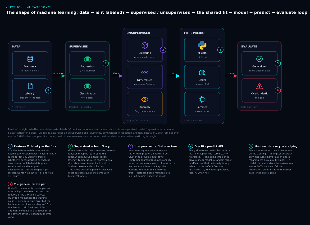
The badges trace the ideas to carry out of this lesson: whether a label y exists is the fork that decides everything (1); supervised learning maps X→y as regression or classification (2); unsupervised learning finds structure in X alone (3); every model shares the one fit/predict API (4); you must score on held-out data or you are only measuring memorization (5); and the gap between train and test error is where underfitting and overfitting live (6).
⚠️ Why you MUST hold out data — and a leakage preview. The test set is sacred: it stands in for “the future,” data the model has never seen. Score on the training set instead and every model looks brilliant, because you are grading the exam with the answer key it studied. Worse is data leakage — when information about the answer sneaks into the features. If you accidentally include a column that is the target in disguise, the model gets a near-perfect score that evaporates in production:
from sklearn.datasets import load_diabetes
X_ok, y = load_diabetes(return_X_y=True)
X_leak = np.column_stack([X_ok, y + rng.normal(0, 1, y.size)])   # a "feature" that IS the target
# ... train/test split, LinearRegression.fit ...
# test R^2 WITH the leaked feature : 0.9998   <- too good to be true
# test R^2 without it              : 0.3594   <- the honest number
A score that looks too good is a symptom to investigate, not celebrate. The full discipline of splitting, cross-validation, and leak-proofing belongs to the metrics-and-validation lesson; for now, the rule is absolute: hold out data, and be suspicious of near-perfect scores.
You score that held-out data with a metric, and the metric depends on the task. You have already seen R² and accuracy; here is the preview map so the names in later lessons land in place — but note the loud warning attached to accuracy, which the lab demonstrates:
| Task | Metric | Range | Reads as | Caveat |
|---|---|---|---|---|
| Regression | RMSE / MAE | 0 → ∞ (lower better) | typical error, in target units | RMSE punishes big misses harder |
| Regression | R² | ≤ 1 (higher better) | fraction of variance explained | can go negative (worse than the mean) |
| Classification | Accuracy | 0 → 1 | fraction correct | ⚠️ lies on imbalanced classes |
| Classification | Precision / Recall | 0 → 1 | of flagged, how many right / of real, how many caught | trade off against each other |
| Classification | F1 | 0 → 1 | harmonic mean of precision & recall | better than accuracy when imbalanced |
| Clustering | Silhouette | −1 → 1 | how well-separated the clusters are | no labels needed |
The model-family map
You have driven a linear model, a logistic classifier, and KMeans. There are dozens more, but they cluster into a handful of families with shared instincts. You do not need the details yet — later lessons take these one at a time — but you should recognise the map so new algorithm names land in the right slot.
| Family | Idea in one line | Examples (sklearn) | Strengths | Watch out for |
|---|---|---|---|---|
| Linear | Fit a weighted sum of features | LinearRegression, LogisticRegression, Ridge, Lasso |
Fast, interpretable, strong baseline | Only linear relationships (unless you add features) |
| Tree-based | Ask yes/no questions, split the data | DecisionTreeClassifier, DecisionTreeRegressor |
Handles non-linearity, no scaling needed, readable | A single deep tree overfits badly |
| Ensembles | Combine many weak models | RandomForest…, GradientBoosting…, HistGradientBoosting… |
Top accuracy on tabular data | Slower, less interpretable |
| Distance-based | Predict from the nearest examples | KNeighborsClassifier, KMeans |
Simple, no training phase (kNN) | Must scale features; slow at prediction; curse of dimensionality |
| Kernel / SVM | Separate classes with a max-margin boundary | SVC, SVR |
Powerful in medium dimensions | Scaling-sensitive; slow on large data |
| Neural networks | Layers of learned non-linear transforms | MLPClassifier; PyTorch/TensorFlow for deep nets |
State of the art on images, text, audio | Hungry for data and compute; opaque |
| Naive Bayes | Probabilities under a “features independent” assumption | GaussianNB, MultinomialNB |
Very fast, great text baseline | The independence assumption is usually false |
One axis the table hides is cost: families differ enormously in how training time and prediction latency scale with the data. A lazy kNN trains instantly but then scans every stored row on each prediction — an O(n) query cost that balloons on big data — while a linear model is the opposite (slow-ish to train, near-instant to predict). Reasoning about that scaling is exactly the Big-O skill from Algorithms: Search, Sort & Complexity, now applied to model choice.
The professional move early on: start with the simplest thing that could work — a linear model or a single tree — as a baseline, then only add complexity if it measurably beats that baseline on held-out data. A random forest that barely edges out LinearRegression is rarely worth the loss of interpretability.
There is a theorem behind this humility, the “no free lunch” result: no single algorithm is best across all possible problems. Which family wins is an empirical question you answer by trying them and comparing on held-out data, not by allegiance. That said, strong priors exist and save time: for tabular data (rows and columns, like most business datasets) gradient-boosted trees — HistGradientBoosting, or libraries like XGBoost and LightGBM — are the usual winners, with a random forest close behind. For images, audio, and text, neural networks dominate and nothing else is close. For a fast, explainable baseline you can defend to a stakeholder, a linear or logistic model is hard to beat. Match the family to the data shape first, then let the held-out score settle the rest.
The end-to-end ML workflow
A model is maybe 10% of a real ML project. The other 90% is the pipeline around it, and beginners who jump straight to fit skip the steps that actually determine success. The honest workflow:
| # | Stage | What you actually do | Where it goes wrong |
|---|---|---|---|
| 1 | Frame the problem | Is this even ML? Regression or classification? What’s the metric of success? | Using ML where a rule fits; optimising the wrong metric |
| 2 | Get & understand data | Collect, inspect, check quality, plot distributions | Non-representative or biased data; too little of it |
| 3 | Clean & engineer features | Handle missing values, encode categories, scale, build features | Leakage; scaling after splitting; garbage features |
| 4 | Split | Hold out a test set (and a validation set / CV) before touching it | Peeking at the test set; splitting after preprocessing |
| 5 | Choose & train a model | Baseline first, then candidates; .fit(X_train, y_train) |
Jumping to complex models; no baseline |
| 6 | Evaluate | Score on held-out data with the right metric; compare to baseline | Evaluating on train; accuracy on imbalanced data |
| 7 | Tune | Adjust hyperparameters via cross-validation | Tuning on the test set (it’s no longer held-out) |
| 8 | Deploy | Ship the model behind an API; version it and the data | Training/serving skew; unversioned models |
| 9 | Monitor | Watch live performance; data drifts, models rot | Assuming a model stays good forever |
Two stages deserve emphasis because they are where beginners bleed. Splitting comes before preprocessing decisions that learn from data — if you scale or select features using the whole dataset and then split, information from the test set has leaked into training. And monitoring is not optional: the world changes, so the pattern your model learned drifts out of date. This has a name — concept drift — and it is not rare. A demand-forecasting model trained on 2019 data was worthless in April 2020; a fraud model degrades the moment fraudsters adapt to it; a recommender trained on last year’s catalogue slowly stops recommending anything people currently want. The model does not announce its own decay — its accuracy just quietly slides while it keeps returning confident predictions. A model that was excellent at launch can silently rot, and the only way you find out is by tracking live performance against fresh labels and alerting when it drops.
Because the split is where so much rides, know its knobs — train_test_split is the one function you will call in every supervised project:
| Parameter | Does | Sensible default |
|---|---|---|
test_size |
fraction (or count) held out for testing | 0.2–0.25 |
random_state |
seeds the shuffle so the split is reproducible | any fixed int (0, 42) |
stratify=y |
keep each class’s proportion equal in train and test | always set for classification |
shuffle |
shuffle before splitting (default True) |
leave True — except for time series |
| return order | X_train, X_test, y_train, y_test |
memorise this order |
⚠️ For time-series data, do not shuffle — you must train on the past and test on the future, or you leak tomorrow into today. Use TimeSeriesSplit instead; a random split on time-ordered data is a classic silent leak.
Data quality dominates: garbage in, garbage out
Here is the least glamorous and most important truth in the field: better data beats a fancier model, almost always. A modest model on clean, representative, well-labeled data will crush a state-of-the-art architecture on biased, mislabeled, or unrepresentative data. Kaggle grandmasters and industry teams spend the majority of their time on data, not models — because that is where the wins are.
The model can only learn what is in the data, faithfully including the mistakes:
| Data problem | What the model learns instead | Symptom | Fix |
|---|---|---|---|
| Mislabeled examples | The wrong answer, confidently | Ceiling on accuracy you can’t break | Audit & relabel; measure label quality |
| Non-representative sample | Patterns of the wrong population | Great offline, fails on real users | Sample to match production reality |
| Missing values, done wrong | Artifacts of your imputation | Weird importance on “was-missing” | Impute deliberately; add missingness flags |
| Imbalanced classes | “Always predict the majority” | High accuracy, catches no positives | Resample, reweight, change the metric |
| Leaked target | The answer via a proxy feature | Suspiciously perfect scores | Audit features; split before engineering |
| Too few examples | The noise, not the signal | High variance, overfits | Get more data; simpler model; regularize |
| Historical bias | Society’s past discrimination | Unfair predictions on protected groups | Audit for bias; curate data; fairness constraints |
⚠️ A model trained on biased data encodes and amplifies that bias, wearing the mask of objectivity. If your hiring data reflects decades of biased human decisions, a model learns to reproduce them — and now the discrimination comes with a veneer of mathematical neutrality that is harder to challenge. ML does not launder bias out of data; it bakes it in. This is not a corner case; it is a first-order responsibility of anyone who ships models.
The honest limits of ML
To use ML well you must be clear-eyed about what it is not, because the hype systematically oversells it. A trained model is a compressed summary of correlations in its training data — a very sophisticated one, but that is the whole of it. From that single fact every limit follows.
- It pattern-matches; it does not reason. A model has no model of the world, no understanding, no common sense. It learns “inputs like these tended to have labels like those” and interpolates. It cannot notice that its answer is absurd, because it has no notion of absurd.
- It learns correlation, never causation. It will exploit any signal that predicts the label — including the ones you did not want. The classic cautionary tale: a model trained to spot cancer in X-rays learned to detect the ruler radiologists place next to suspected tumours, because suspicious scans got measured. It “worked” in testing and would have been useless (and dangerous) in the clinic. High accuracy is not understanding.
- It only knows its training distribution. Ask a model about inputs unlike anything it trained on and it does not say “I don’t know” — it confidently extrapolates nonsense. The degree-15 polynomial flinging off to ±2 between training points is this failure in miniature.
- It inherits and amplifies the data’s bias, as above, with a false air of neutrality.
- It is opaque by default. A random forest or neural net cannot, unaided, tell you why it decided what it did. Explainability is a whole separate discipline you bolt on; it does not come free.
- It rots. The world drifts away from the training data (new fraud patterns, new slang, a changed market), and a model that was excellent silently degrades. Yesterday’s fit is not tomorrow’s.
| People assume ML… | Reality |
|---|---|
| understands the problem | matches patterns in past data, nothing more |
| finds causes | finds correlations — including spurious ones |
| is objective / neutral | reflects the biases baked into its training data |
| works on any input | only trustworthy within its training distribution |
| can explain itself | opaque unless you add explainability tooling |
| stays good once trained | drifts and rots as the world changes |
| replaces domain expertise | needs it more than ever — to frame, check, and catch it |
None of this means ML is not extraordinarily useful — it is, for exactly the problems in this lesson’s opening. It means you deploy it as a fallible statistical tool with measured error rates and human oversight, not an oracle. The engineers who get burned are the ones who forgot it was correlation all the way down.
Hands-on lab
Run the full arc on scikit-learn’s built-in datasets — no downloads, they ship with the library — then reproduce the overfitting curve yourself and save the figure headless. Everything is seeded; your numbers will match the comments.
scikit-learn bundles small “toy” datasets (loaded with load_*) and synthetic-data generators (make_*) precisely so you can practise without hunting for data. The ones worth knowing:
| Loader | Task | Shape | Classes / target | Use for |
|---|---|---|---|---|
load_diabetes() |
regression | 442 × 10 | continuous 25–346 | a realistic (hard) regression |
load_iris() |
classification | 150 × 4 | 3 balanced (50 each) | the classic first classifier |
load_wine() |
classification | 178 × 13 | 3 (59/71/48) | near-separable, easy win |
load_breast_cancer() |
classification | 569 × 30 | 2 (binary) | binary, mildly imbalanced |
make_blobs(...) |
clustering | you choose | you choose the centers | clean clustering demos |
make_classification(...) |
classification | you choose | you choose | stress-testing / imbalance |
Setup (once):
python3 -m venv .venv && source .venv/bin/activate    # Windows: .venv\Scripts\activate
pip install scikit-learn numpy pandas matplotlib
Put each step in ml_lab.py and run with python ml_lab.py.
Step 1 — regression on the diabetes dataset (and a baseline).
import numpy as np
from sklearn.datasets import load_diabetes
from sklearn.linear_model import LinearRegression
from sklearn.dummy import DummyRegressor
from sklearn.model_selection import train_test_split
from sklearn.metrics import mean_absolute_error, r2_score

dia = load_diabetes()
print("X shape:", dia.data.shape)                 # => X shape: (442, 10)
print("features:", dia.feature_names)             # age, sex, bmi, bp, s1..s6
X_tr, X_te, y_tr, y_te = train_test_split(dia.data, dia.target, test_size=0.25, random_state=0)

reg = LinearRegression().fit(X_tr, y_tr)
pred = reg.predict(X_te)
print("test R^2 :", round(r2_score(y_te, pred), 4))                 # => 0.3594
print("test MAE :", round(mean_absolute_error(y_te, pred), 2))      # => 45.12

baseline = DummyRegressor(strategy="mean").fit(X_tr, y_tr)          # always predict the mean
print("baseline MAE:", round(mean_absolute_error(y_te, baseline.predict(X_te)), 2))  # => 58.31
What just happened: a real regression. R²=0.36 is modest — real medical data is hard, and that honesty is the point; ML is not magic. But the model’s MAE (45.1) clearly beats the dumb “predict the mean” baseline (58.3), so it has learned something real. Always compute the baseline — a model that cannot beat it is worthless, however sophisticated.
Step 2 — classification on the wine dataset.
from sklearn.datasets import load_wine
from sklearn.ensemble import RandomForestClassifier
from sklearn.metrics import accuracy_score, confusion_matrix

wine = load_wine()
print("X shape:", wine.data.shape, "classes:", wine.target_names.tolist())
# => X shape: (178, 13) classes: ['class_0', 'class_1', 'class_2']
print("class counts:", np.bincount(wine.target).tolist())          # => [59, 71, 48]

X_tr, X_te, y_tr, y_te = train_test_split(
    wine.data, wine.target, test_size=0.25, random_state=0, stratify=wine.target)
clf = RandomForestClassifier(n_estimators=100, random_state=0).fit(X_tr, y_tr)

print("train accuracy:", round(clf.score(X_tr, y_tr), 4))          # => 1.0
print("test  accuracy:", round(accuracy_score(y_te, clf.predict(X_te)), 4))  # => 1.0
print("confusion matrix:\n", confusion_matrix(y_te, clf.predict(X_te)))
# => [[15  0  0]
#     [ 0 18  0]
#     [ 0  0 12]]
What just happened: a 3-class classifier. Wine is nearly separable, so the forest hits 100% on the held-out set — the confusion matrix is perfectly diagonal (every true class predicted correctly, zero off-diagonal mistakes). Note stratify=wine.target, which keeps the class proportions identical in train and test — essential when classes are uneven. Do not expect 100% on real problems; wine is a gentle teaching set.
Step 3 — clustering on blobs, and choosing k (elbow + silhouette).
from sklearn.datasets import make_blobs
from sklearn.cluster import KMeans
from sklearn.metrics import silhouette_score

X, _ = make_blobs(n_samples=300, centers=3, cluster_std=1.0, random_state=42)
# We deliberately IGNORE the true labels (the _) — clustering is unsupervised.

for k in range(2, 7):
    km = KMeans(n_clusters=k, n_init=10, random_state=0).fit(X)
    sil = silhouette_score(X, km.labels_)          # needs >= 2 clusters
    print(f"k={k}: inertia={km.inertia_:8.1f}  silhouette={sil:.3f}")
# => k=2: inertia=  5763.5  silhouette=0.705
# => k=3: inertia=   566.9  silhouette=0.848   <- inertia elbow AND silhouette peak
# => k=4: inertia=   496.8  silhouette=0.660
# => k=5: inertia=   426.3  silhouette=0.492
# => k=6: inertia=   361.1  silhouette=0.331
What just happened: two independent ways to choose k agree on 3. Inertia (total within-cluster distance) always falls as k rises — with k=n every point is its own cluster and inertia hits zero, which is useless as a target — so you look for the elbow, the sharp bend where the drop flattens (here the plunge to k=3 then the flattening after). The silhouette score (−1 to 1, higher = better-separated clusters) needs no such eyeballing: it peaks cleanly at k=3 (0.848). We built three blobs, so both are right. Choosing k is the hard part of KMeans:
| Method | What it measures | Best k is where… |
On our blobs |
|---|---|---|---|
| Elbow (inertia) | within-cluster tightness | the curve bends / flattens | k=3 (bend) |
| Silhouette | separation vs cohesion, per point | the score is highest | k=3 (0.848) |
| Domain knowledge | what the clusters are for | the business says so | “we want 3 tiers” |
Step 4 — demonstrate overfitting yourself and save the figure.
import matplotlib
matplotlib.use("Agg")                              # headless: render without a screen
import matplotlib.pyplot as plt
from sklearn.pipeline import make_pipeline
from sklearn.preprocessing import PolynomialFeatures
from sklearn.model_selection import train_test_split
from sklearn.metrics import mean_squared_error

rng = np.random.default_rng(1)
x = np.sort(rng.uniform(0, 1, size=30))
y = np.cos(1.5 * np.pi * x) + rng.normal(0, 0.12, size=30)
X = x.reshape(-1, 1)
X_tr, X_te, y_tr, y_te = train_test_split(X, y, test_size=0.4, random_state=1)

degrees = range(1, 16)
train_err, test_err = [], []
for d in degrees:
    m = make_pipeline(PolynomialFeatures(d), LinearRegression()).fit(X_tr, y_tr)
    train_err.append(np.sqrt(mean_squared_error(y_tr, m.predict(X_tr))))
    test_err.append(np.sqrt(mean_squared_error(y_te, m.predict(X_te))))

best = list(degrees)[int(np.argmin(test_err))]
print("lowest test RMSE at degree", best)          # => lowest test RMSE at degree 3

plt.figure(figsize=(7, 4.5))
plt.plot(list(degrees), train_err, "o-", label="train RMSE")
plt.plot(list(degrees), test_err, "s-", label="test RMSE (held-out)")
plt.axvline(best, ls=":", color="green", label=f"best (deg {best})")
plt.yscale("log"); plt.xlabel("polynomial degree"); plt.ylabel("RMSE (log)")
plt.title("Train falls forever; test is a U — the generalization gap")
plt.legend(); plt.tight_layout()
plt.savefig("overfit.png", dpi=110)
print("saved -> overfit.png")
What just happened: you generated the U-curve on your own machine. Open overfit.png: the train line slides down monotonically while the test line dips to a minimum at degree 3 and then climbs steeply. That divergence is overfitting, and you can only see it because you held out a test set. ⚠️ matplotlib.use("Agg") before importing pyplot is what lets this run on a headless server (no display); plotting itself is covered in Matplotlib: Plotting Basics.
Step 5 — the imbalanced-accuracy trap (a preview of why accuracy lies).
from sklearn.dummy import DummyClassifier
from sklearn.metrics import accuracy_score, balanced_accuracy_score, f1_score

y_imb = np.zeros(1000, dtype=int); y_imb[:50] = 1     # 5% positive (fraud-like)
rng.shuffle(y_imb)
Xz = np.zeros((1000, 1))
dummy = DummyClassifier(strategy="most_frequent").fit(Xz, y_imb)
pred = dummy.predict(Xz)
print("accuracy         :", round(accuracy_score(y_imb, pred), 4))          # => 0.95
print("balanced accuracy:", round(balanced_accuracy_score(y_imb, pred), 4)) # => 0.5
print("F1 (positive)    :", round(f1_score(y_imb, pred), 4))                # => 0.0
What just happened: a model that always predicts “not fraud” scores 95% accuracy on data that is 95% negative — while catching zero actual fraud (F1 = 0, balanced accuracy = 0.5, no better than a coin). Accuracy is a liar on imbalanced data. Which metric to trust, and why, is the heart of the metrics lesson; the lesson here is that a single number is never enough.
Common mistakes and troubleshooting
| Symptom / mistake | Cause | Fix |
|---|---|---|
| Chose ML for a task with a known rule | ML fashion over judgement | If you can state the rule, write the rule — it’s exact, fast, explainable |
ValueError: Expected 2D array, got 1D array instead |
Passed a flat list/1-D array as X |
X must be 2-D: X.reshape(-1, 1) for one feature, reshape(1, -1) for one sample |
| 100% train accuracy, poor test accuracy | Overfitting — model memorized noise | Simpler model, more data, regularization; trust the held-out score |
| Both train and test accuracy poor | Underfitting — model too simple | More complex model / better features; more capacity |
| “Amazing” accuracy you can’t reproduce live | Evaluated on the training data | Always score on a held-out test set — training score is meaningless |
| Model looks great but nobody knows if it’s good | No baseline to compare against | Compare to DummyClassifier/DummyRegressor; beat it or it’s worthless |
| 95% accuracy, catches none of the rare class | Imbalanced classes fool accuracy | Use balanced accuracy / precision-recall / F1; resample or reweight |
| Test score suspiciously near-perfect | Data leakage — a feature encodes the target | Audit features; split before preprocessing; drop target-derived columns |
| High variance, wildly different each run | Too little data for the model’s complexity | Get more data, simplify the model, add regularization |
| Great in dev, fails on real users | Non-representative training data | Sample to match production; check for distribution shift |
| Clusters make no sense / one feature dominates | Clustering without scaling | StandardScaler before any distance-based method (KMeans, kNN, SVM) |
| “X causes Y because they correlate” | Confused correlation with causation | Correlation is a hint, never proof; ML finds patterns, not causes |
NotFittedError on .predict |
Called .predict before .fit |
Fit first: model.fit(X, y) then model.predict(X_new) |
Found input variables with inconsistent numbers of samples: [n, m] |
X and y have different lengths |
len(X) == len(y) — one label per row |
The three that do the most silent damage, in prose:
Evaluating on the training set is the original sin, because it always looks like success. Every model, no matter how bad, scores better on data it trained on than on new data — often perfectly, if it is flexible enough to memorize. So the training score is not a measure of quality; it is a measure of memorization capacity. Beginners fit a model, print .score(X_train, y_train), see 0.99, and ship. Then production accuracy is 0.7 and nobody understands why. The habit that saves you: the first number you look at is always the held-out score, and you never, ever tune against the test set (the moment you make decisions based on it, it stops being held-out and you need a fresh one).
Overfitting and underfitting look identical from inside the model — you need the two-number diagnosis. A single accuracy figure cannot tell you which failure you have; you must compare train vs test. Both high → underfitting (add capacity). Train low, test high → overfitting (remove capacity or add data). Train and test both low and close → you are done. Print both numbers, always, and read the gap — the gap between them is the single most informative diagnostic in applied ML, and it is one subtraction.
Forgetting to scale before distance-based methods silently corrupts the result. KMeans, kNN, and SVM measure distances between rows, and distance is dominated by whichever feature has the biggest units. Cluster on {age: 0–100, income: 0–100000} without scaling and the algorithm effectively ignores age — income’s thousands drown age’s tens in the Euclidean distance. We can measure the damage: cluster data whose true structure lives in a small-scale feature while a large-scale noise feature sits alongside, and score against the true labels with the Adjusted Rand Index (1.0 = perfect, 0 = random):
# true groups live in a small-range feature; a huge-range NOISE feature sits beside it
# ARI raw (unscaled) : -0.0034   <- recovers NOTHING; the noise feature hijacks distance
# ARI scaled         :  1.0000   <- StandardScaler first restores the real structure
Unscaled, the clustering recovers nothing (ARI ≈ 0); scaling first recovers the true groups perfectly (ARI = 1.0). The fix is one line — StandardScaler().fit_transform(X) before you cluster — and forgetting it is one of the most common reasons “my clusters look random.”
Cheat-sheet
| Task | Code | Note |
|---|---|---|
| Feature matrix / labels | X (2-D, n×d), y (1-D, n) |
uppercase X, lowercase y |
| Fix 1-D X | X.reshape(-1, 1) |
one feature per column |
| Train/test split | train_test_split(X, y, test_size=0.25, random_state=0) |
hold out before touching |
| Stratified split | train_test_split(..., stratify=y) |
keep class balance |
| Fit a model | model.fit(X_train, y_train) |
learn from data |
| Predict | model.predict(X_new) |
apply the function |
| Class probabilities | clf.predict_proba(X) |
confidence, not just label |
| Cluster (no labels) | KMeans(n_clusters=k, n_init=10, random_state=0).fit(X) |
.labels_, .cluster_centers_, .inertia_ |
| Linear regression | LinearRegression() |
.coef_, .intercept_ |
| Logistic (classifier!) | LogisticRegression() |
despite the name, classification |
| Random forest | RandomForestClassifier(n_estimators=100, random_state=0) |
strong tabular baseline |
| Scale features | StandardScaler().fit_transform(X) |
before kNN / KMeans / SVM |
| Regression metrics | r2_score, mean_absolute_error, mean_squared_error |
R², MAE, MSE |
| Classification metrics | accuracy_score, f1_score, confusion_matrix |
accuracy lies on imbalance |
| Baseline | DummyRegressor(strategy="mean") / DummyClassifier(strategy="most_frequent") |
beat it or it’s worthless |
| Built-in datasets | load_diabetes(), load_wine(), load_iris(), make_blobs() |
no download |
| Overfit signature | train ↓, test ↑ | compare the two numbers |
| Reproducible RNG | np.random.default_rng(seed) |
seed everything |
| Headless plot | matplotlib.use("Agg") before import pyplot |
save, don’t show |
Interview and exam questions
Q: In one sentence, what is machine learning, and how does it differ from ordinary programming? A: Machine learning learns a function from example data instead of having it programmed by hand — ordinary programming is “rules in, answers out” (you write the logic), while ML is “data and answers in, rules out” (the algorithm infers the logic from labeled examples). It is the right tool precisely when the rule is unknown or too complex to write by hand, like recognizing faces or detecting spam.
Q: Give a task where you should NOT use machine learning, and say why.
A: Anything with a known, exact rule — computing tax, checking age >= 18, validating a credit-card number with the Luhn checksum, deciding free shipping over a threshold. A hand-written rule is exact, instant, explainable, needs no training data, and never drifts; an ML model for the same job is approximate, needs data, can fail on unseen inputs, and is a black box. Using ML there is strictly worse than an if statement.
Q: Explain supervised vs unsupervised learning, and the two kinds of supervised.
A: Supervised learning has labeled data — every training row includes the answer y — and learns to predict it; it splits into regression (continuous target: price, latency) and classification (discrete target: spam/not, which class). Unsupervised learning has no labels, only X, and finds structure instead: clustering (group similar rows), dimensionality reduction (compress features), and anomaly detection (flag outliers).
Q: What are X and y, and what shapes does scikit-learn expect?
A: X is the feature matrix — 2-D, shape (n_samples, n_features), one row per example and one column per feature. y is the target vector — 1-D, shape (n_samples,), one label per row. Passing a 1-D array as X raises ValueError: Expected 2D array, got 1D array instead; the fix is X.reshape(-1, 1) for a single feature.
Q: What is overfitting, what is underfitting, and how do you tell them apart? A: Underfitting is a model too simple to capture the signal — it has high error on both training and test data. Overfitting is a model so flexible it memorizes the training noise — very low training error but high test error. You distinguish them by comparing the two numbers: both high → underfit; train low and test high → overfit; both low and close → just right. The gap between train and test error is the diagnostic.
Q: Why must you evaluate on held-out data? What goes wrong if you don’t? A: Because the goal is generalization to unseen data, and a model always scores better — often perfectly — on data it trained on, since it can memorize. Evaluating on the training set measures memorization, not quality, so every model looks great and you ship one that fails in production. You hold out a test set that stands in for “the future” and never make decisions based on it (or it stops being held-out).
Q: Describe the bias–variance tradeoff and how it relates to the U-shaped test-error curve. A: Expected error on new data decomposes into bias (error from too-simple assumptions — underfitting), variance (error from over-sensitivity to the training sample — overfitting), and irreducible noise. Simple models have high bias and low variance; complex models the reverse. As complexity rises, bias falls and variance grows, so total error traces a U — minimised at the sweet spot. In the polynomial demo, degree 1 was high-bias (underfit), degree 15 high-variance (overfit), and degree 3 sat at the bottom of the U.
Q: A classifier reports 97% accuracy on a dataset that is 97% one class. Is it good?
A: Almost certainly not — a model that blindly predicts the majority class scores 97% while catching none of the rare class. Accuracy is misleading on imbalanced data. Look at balanced accuracy, precision, recall, or F1 on the minority class, and compare to a DummyClassifier(strategy="most_frequent") baseline; if it doesn’t beat that, it has learned nothing useful.
Q: What is data leakage and how does it show up? A: Leakage is when information about the target sneaks into the features — for example a column derived from the label, or preprocessing (scaling, feature selection) done on the whole dataset before splitting. It shows up as a suspiciously high, “too good to be true” score that collapses in production, because the model was quietly given the answer. Prevent it by splitting before any data-dependent preprocessing and auditing features for target-derived columns.
Q: Why must you scale features before KMeans or kNN, but not (usually) before a decision tree?
A: KMeans, kNN, and SVM measure distances between rows, and distance is dominated by the feature with the largest units — an unscaled large-range feature drowns out small-range ones. Scaling (e.g. StandardScaler) puts features on comparable footing. Trees split one feature at a time on thresholds, so they are invariant to feature scale and don’t need it. Skipping scaling before distance methods can make clustering recover essentially nothing (ARI ≈ 0 vs 1.0 scaled).
Q (coding): Fit a model, and report train and test scores to diagnose over/underfitting. A:
from sklearn.model_selection import train_test_split
X_tr, X_te, y_tr, y_te = train_test_split(X, y, test_size=0.25, random_state=0)
model.fit(X_tr, y_tr)
train_score = model.score(X_tr, y_tr)
test_score  = model.score(X_te, y_te)
print(f"train={train_score:.3f}  test={test_score:.3f}  gap={train_score-test_score:.3f}")
# both low  -> underfit ; train high & test low -> overfit ; both high & close -> good
The gap is the headline: a large positive gap means overfitting, both-low means underfitting.
Q: Why is “better data beats a better model” usually true? A: A model can only learn what’s in the data — it faithfully reproduces mislabeled rows, unrepresentative samples, and historical bias. A modest model on clean, representative, correctly labeled data outperforms a sophisticated one on flawed data, and no architecture fixes garbage inputs (garbage in, garbage out). That’s why practitioners spend most of their time on data collection, cleaning, and labeling, not model selection.
Q: Is a strong correlation or a high-accuracy model evidence that one thing causes another?
A: No. ML is correlation-based pattern-matching; it learns what predicts the label, not what causes it. A model can predict drownings from ice-cream sales (summer drives both) without any causal link. Predictive power is not causal proof — establishing causation needs controlled experiments or careful causal inference, not a good .score().
Key takeaways
- ML learns a function from data instead of hand-coding rules — use it when the rule is unknown or too complex to write; if you can state the rule (tax, eligibility, thresholds), write the rule, because it’s exact, fast, and explainable.
- The vocabulary is
X(2-D feature matrix,n×d) andy(1-D labels,n). Supervised learning mapsX→y(regression for a number, classification for a class); unsupervised learning finds structure inXalone (clustering, dimensionality reduction, anomaly detection). - scikit-learn is one uniform API:
.fit(X, y)to learn,.predict(X_new)to apply,.predict_probafor confidence — the same three lines drive a linear model, a forest, or KMeans. - Generalization is the whole game. A model must work on data it never saw, so you must hold out a test set. Training-set scores measure memorization and are meaningless as a quality signal.
- Overfitting (train low, test high) vs underfitting (both high) is diagnosed by comparing two numbers. The bias–variance tradeoff traces a U-shaped test-error curve; you want the bottom — degree 3, not degree 1 or 15.
- Always beat a baseline (
DummyRegressor/DummyClassifier), and never trust accuracy alone on imbalanced data — 95% accuracy can catch zero of the rare class. - Scale features before distance-based methods (KMeans, kNN, SVM) or a big-unit feature hijacks the result; audit for data leakage when a score looks too good.
- Data quality dominates modeling — better data beats a fancier model — and ML is honest but limited: it pattern-matches from correlations, needs representative data, encodes whatever bias the data carries, and does not reason or know cause from coincidence.