There is a moment, a few weeks after you write a good analysis, when someone asks for it again. Not the code — the answer. “What did last month’s cloud spend look like, broken down by service?” And you realise the notebook that produced it is three laptops and one pip upgrade ago, half its cells were run out of order, the CSV it read has been overwritten, and the number you confidently quoted in a meeting can no longer be reproduced by anyone, including you.
That gap — between an analysis that ran once, by hand, and happened to be right and one that runs every morning, unattended, and stays right — is what a data pipeline closes. It is not a bigger script. It is a different kind of software, with different obligations: it must be reproducible, it must be scheduled, it must be monitored, and it must fail loudly when the data is wrong rather than quietly shipping a beautiful, incorrect chart.
Everything below was built and executed on Python 3.12.3 with pandas 3.0.3, pyarrow 25.0.0, jinja2 3.1.6 and streamlit 1.59.2 — real data, real output, real failures. We build a small cloud-cost ETL pipeline, watch its quality gate reject a poisoned row and refuse to write anything, measure exactly how much Parquet beats CSV, generate a templated HTML report, and serve a Streamlit dashboard over the result.
Why this matters
A one-off analysis and a pipeline solve the same problem once. Then they diverge, and every way they diverge is a 3am phone call waiting to happen.
The one-off ran in your notebook because you were there: you noticed the empty file, you re-ran the cell, you eyeballed the total and thought “that looks about right.” A pipeline has none of that. It runs at 03:00 while you sleep, on a machine you’re not watching, against data an upstream team changed without telling you. Nobody is going to eyeball anything. So every check you used to do with your eyes has to become code, or it doesn’t happen.
Here is the shape of the difference, and it’s the whole lesson in one table:
| One-off analysis | Pipeline | What changes |
|---|---|---|
| You run it | A scheduler runs it | No human sees the failure first |
| You spot the bad row | An assertion must catch it | Validation becomes code, or it’s absent |
| “Looks about right” | Row-count + freshness checks | Sanity becomes a monitored number |
| Overwrites the CSV | Immutable, dated outputs | You can reproduce last month |
| Cells run in click-order | A main() runs top-to-bottom |
Hidden state can’t hide |
| Re-run = maybe different | Re-run = identical (idempotent) | A retry after a crash is safe |
| Types live in your head | Types live in Parquet | The schema survives the handoff |
The mental model to hold for the rest of the lesson: a pipeline is a chain of verbs — extract, transform, validate, load — wrapped in two disciplines the notebook didn’t need. The first discipline is a gate: nothing gets loaded until it’s proven clean, because the one thing worse than a pipeline that crashes is a pipeline that succeeds with wrong data. The second is observability: every run leaves a receipt — how many rows in, how many out, how many rejected, how long it took — so a run that quietly did nothing is a page you get, not a surprise a user finds three days later.
What a data pipeline actually is
Strip away the tooling and a pipeline is four verbs and two promises.
The four verbs are Extract (get the raw data out of wherever it lives — a CSV export, an API, a database), Transform (parse it into real types, derive the columns you need, join in reference data), Validate (prove it meets your quality bar), and Load (write the result somewhere durable and queryable). You will see this written ETL. The verbs are stable; only their order and where the transform runs change.
| Verb | Owns | Must NOT | Failure if skipped |
|---|---|---|---|
| Extract | Pulling raw bytes from source, unchanged | Clean or reshape (that hides where bad data came from) | You can’t tell source errors from your own |
| Transform | Typing, deriving, joining reference data | Aggregate before validation runs | A null dimension gets summed into a phantom group |
| Validate | Proving the batch meets the quality bar | Let a bad row through “just this once” | A wrong report that looks right |
| Load | Writing durable, queryable, idempotent output | Append (it doubles on re-run) | Re-runs corrupt the data |
The two promises are idempotent (running it twice produces the same result as running it once — no duplicates, no drift) and observable (every run is monitored for freshness and volume, so silent failure is impossible). Those two words carry more weight than all the tooling, and most pipeline pain traces back to skipping one of them.
| Property | What it means | What breaks without it |
|---|---|---|
| Reproducible | Same input → same output, on any machine | “It worked on the old server”; numbers you can’t defend |
| Scheduled | A clock triggers it, not a human | It runs when someone remembers, i.e. not reliably |
| Idempotent | Re-running is safe and identical | A retry after a crash doubles every row |
| Observable | Each run emits freshness + volume metrics | A run that produced nothing looks exactly like success |
| Fails loud | Bad data aborts or is quarantined + alerted | A wrong report that looks right, found weeks later |
ETL vs ELT — the order of two letters
The industry argues about ETL versus ELT, and the difference is genuinely just when you transform.
ETL transforms before loading: extract the raw data, clean and reshape it in your Python process (or a tool), then load the finished, typed result into the destination. That’s what this lesson builds, and it’s the right default when your destination is a file store or a modest database and your transforms are Python-shaped.
ELT loads first, raw, into a powerful warehouse (BigQuery, Snowflake, Redshift, Databricks), then transforms inside the warehouse using SQL — typically with a tool like dbt. It wins when the data is huge and the warehouse is more powerful than your one machine: you let the warehouse’s distributed engine do the heavy lifting instead of pulling terabytes through pandas.
| ETL | ELT | |
|---|---|---|
| Transform runs | In your process, before load | In the warehouse, after load |
| Destination holds | Only clean, finished data | Raw data and transformed views |
| Best when | Modest volume; Python transforms; file/DB target | Huge volume; a powerful cloud warehouse; SQL transforms |
| Typical stack | Python + pandas + Parquet/Postgres | BigQuery/Snowflake + dbt |
| Reprocess history | Re-run the transform code | Re-run SQL over already-loaded raw |
| This lesson | ✅ we build this | Mentioned; the concepts transfer |
Neither is more advanced. ELT became popular because cloud warehouses got cheap and absurdly powerful, making “just load everything raw and sort it out in SQL” viable at scales where pulling the data into one Python process would fall over. At our scale — tens of thousands to millions of rows on one box — ETL in Python is exactly right.
Structuring a pipeline as real Python
The single biggest upgrade from notebook to pipeline is boring: it becomes ordinary Python — functions, modules, a main(), and configuration kept out of the code. Each verb is a function with a clear input and output; main() calls them in order and owns the error handling. That structure is what makes a pipeline testable, schedulable, and debuggable at 3am.
Here is the skeleton every function in this lesson hangs on — the same discipline as any installable tool, so it ties directly to Project Structure, Packaging & Documentation (the pipeline is just a package with a main, and [project.scripts] turns it into a schedulable command):
def extract_csv(path): ...      # raw text in
def extract_api(): ...          # reference data
def transform(raw, meta): ...   # parse types, derive, enrich
def validate(df): ...           # the quality gate — raises on bad data
def aggregate(clean): ...       # serving summaries
def load(clean, summaries): ... # write Parquet + SQLite (idempotent)

def run():                      # orchestrate; own the errors + timing
    raw = extract_csv(cfg.raw_csv)
    typed = transform(raw, extract_api())
    clean = validate(typed)     # nothing past here is unclean
    load(clean, aggregate(clean))
The diagram below is the whole pipeline, and it’s the map for the rest of the lesson. Read it left to right: raw sources feed extract and transform, then everything funnels through the validate gate — the red junction where the bad row dies — before a single byte is loaded. Load writes typed Parquet facts and idempotent SQLite serving tables and drops a run manifest; only then do the read-only outputs (the HTML report, the Streamlit dashboard) get built. Scheduling drives it from the left (badge 1); monitoring watches it from the manifest (badge 6).
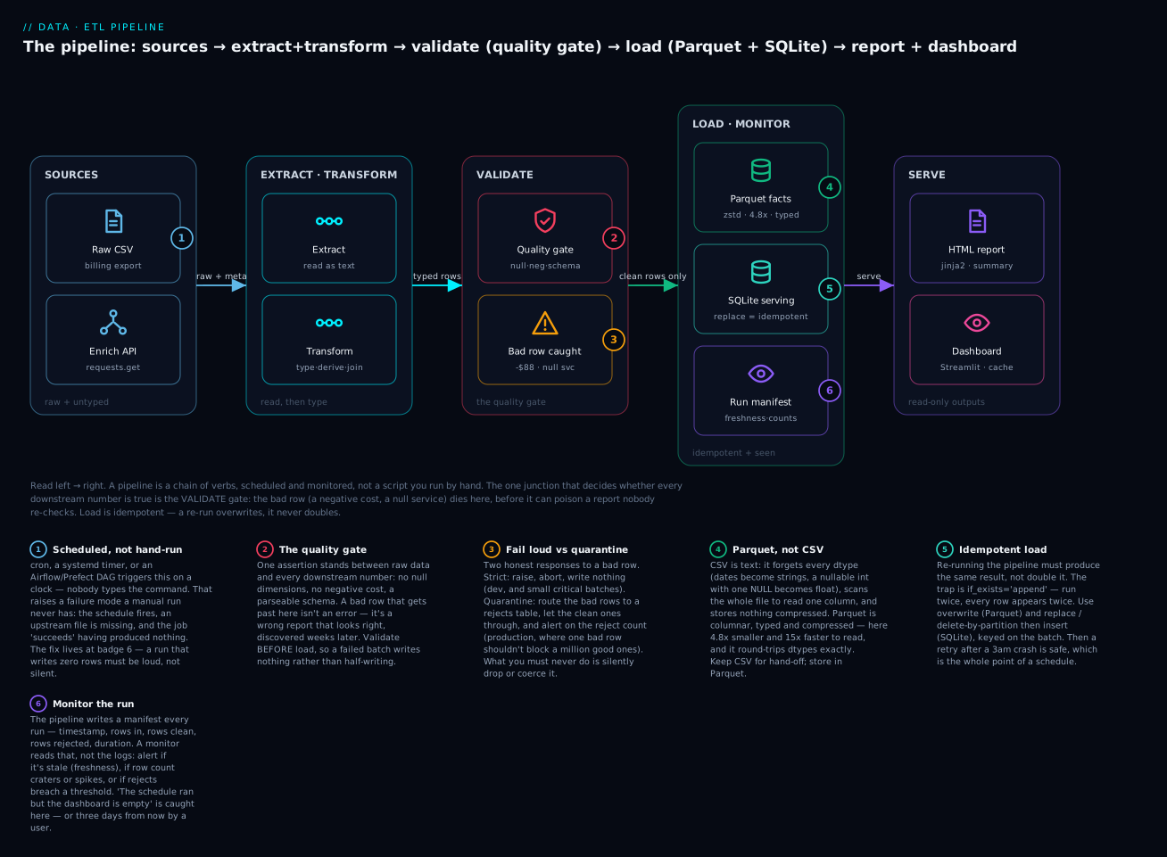
The badges mark the six things that separate a pipeline from a script: it’s triggered by a schedule, not a hand (1); a quality gate stands between raw data and every downstream number (2); a bad row is failed loudly or quarantined-and-alerted, never silently dropped (3); results land in typed columnar Parquet, not lossy CSV (4); the load is idempotent so a retry can’t double your data (5); and every run is monitored so “it ran but produced nothing” is caught in minutes, not days (6).
Config belongs outside the code
The notebook hard-codes "data/usage.csv" in nine cells. The pipeline puts every path, every threshold, every connection string in one config object, separate from the logic — so you can point it at a test fixture, change an output location, or tune a threshold without touching a single function.
from dataclasses import dataclass
from pathlib import Path

@dataclass(frozen=True)
class Config:
    raw_csv: Path = Path("raw/usage_2026_q2.csv")
    fact_parquet: Path = Path("warehouse/facts/usage.parquet")
    sqlite_db: Path = Path("warehouse/cloudcost.db")
    dimensions: tuple[str, ...] = ("date", "service", "region", "account_id")
In production this comes from a TOML file, environment variables, or a secrets manager — never literals scattered through the code, and never a password in the source (that’s a job for env vars, as the database lesson covers). frozen=True makes it read-only: config is set once at startup, not mutated mid-run.
| Belongs in config | Belongs in code |
|---|---|
| File paths, output locations | The transform logic |
| Connection strings, credentials (via env) | The validation rules’ structure |
| Thresholds (max reject %, min rows) | How a threshold is checked |
| Schedule, date range, environment | The order of the verbs |
| Feature flags (strict vs quarantine) | Everything else |
Idempotency: why re-running must be safe
Idempotent means running the pipeline twice yields the same result as running it once. This is not a nicety — it’s the property that makes a schedule survivable. Schedulers retry. Crashes happen mid-run. You will backfill last week. Every one of those re-runs the pipeline over data it has already seen, and if that doubles your numbers, your pipeline is a liability.
The classic way to break idempotency is to append. Watch it happen — the same summary written twice with if_exists="append":
APPEND anti-pattern (if_exists='append')
  after run 1: 8 rows   after identical re-run: 16 rows  <- DUPLICATED (non-idempotent)
Eight rows became sixteen, and nobody raised an error. The fix is to make load replace or overwrite, keyed on what the batch covers, so a re-run supersedes the previous run rather than adding to it.
| Load strategy | Idempotent? | Use when |
|---|---|---|
append |
❌ No — re-run duplicates | Almost never for a scheduled batch |
| Overwrite the whole output | ✅ Yes | Full loads; small/medium data |
replace a table |
✅ Yes | Serving summaries you rebuild each run |
| Delete-then-insert per partition | ✅ Yes | Incremental loads by date |
Upsert / INSERT … ON CONFLICT / MERGE |
✅ Yes | Row-level updates keyed on a primary key |
Full vs incremental loads
A full load reprocesses everything every run. It’s dead simple and idempotent by construction (you overwrite the lot), and it’s the right choice until “everything” stops fitting in your time or memory budget.
An incremental load processes only what’s new or changed since the last run, tracked by a high-water mark — the maximum timestamp or id you’ve already loaded. It’s cheaper at scale but buys you two hard problems: late-arriving data (a row for Monday that shows up Wednesday) and idempotency (you must be able to reprocess a window without duplicating it, which is why incremental loads lean on partition-overwrite or upsert, never append).
| Full load | Incremental load | |
|---|---|---|
| Processes | All data, every run | Only new/changed since a watermark |
| Cost | Grows with total data | Grows with new data |
| Idempotency | Free (overwrite) | Must be engineered (upsert / partition swap) |
| Late data | Handled automatically (reprocesses all) | Needs a lookback window |
| Complexity | Low | Higher — track the watermark, handle gaps |
| Start with | ✅ This, until it hurts | When full loads blow the budget |
Start full. Move to incremental only when a full load no longer fits the clock or the RAM — and when you do, reach for partition-overwrite (delete the day, re-insert the day) so each run stays idempotent.
The quality gate: validate before you load
This is the most important section in the lesson, because it’s the one thing a notebook almost never has and a pipeline cannot live without.
Here is the failure it prevents. Your pipeline reads a billing export. One row has a cost of -88.40 (a glitch in the upstream system) and another has an empty service field (a dropped dimension). Without a gate, both flow straight into your aggregation: the negative cost quietly understates a total, and the null service either crashes a groupby or — worse — silently becomes its own phantom category. The report renders. It looks fine. It is wrong. And because nothing errored, you find out weeks later when someone reconciles against the invoice.
A quality gate is an explicit checkpoint between transform and load that proves the data meets your bar and stops the pipeline if it doesn’t. The rule is: validate before you load, so a failed batch writes nothing rather than half-writing garbage.
What to check
Data-quality checks fall into a small number of families. You won’t need all of them every time, but you should consciously decide which apply.
| Check family | Question it answers | Example |
|---|---|---|
| Not-null | Are required dimensions present? | service, region, date never null |
| Range / sign | Are numbers physically possible? | cost_usd >= 0; 0 <= usage_hours <= 24 |
| Type / parse | Did every value parse? | No NaN left after to_numeric |
| Schema | Right columns, right dtypes? | Exactly these 7 columns, these types |
| Uniqueness | Any duplicate keys? | One row per (date, service, region, account) |
| Referential | Do foreign keys resolve? | Every service exists in the metadata table |
| Volume | Is the row count sane? | Between 40k and 90k rows, not 12 |
| Freshness | Is the data recent enough? | Max date within the last 2 days |
The cheapest gate is a plain assert or an if … raise. Here’s the core of ours — a function that returns a boolean mask of bad rows and logs every rule that fired:
def check_quality(df):
    bad = pd.Series(False, index=df.index)
    null_dims = df[list(cfg.dimensions)].isna().any(axis=1)
    if null_dims.any():
        log.warning("quality: %d rows with a null dimension", int(null_dims.sum()))
        bad |= null_dims
    neg_cost = df["cost_usd"] < 0
    if neg_cost.any():
        log.warning("quality: %d rows with negative cost_usd", int(neg_cost.sum()))
        bad |= neg_cost
    return bad
Fail loud, or quarantine — never silently drop
When the gate finds bad rows, you have exactly three options, and one of them is wrong.
Fail loud raises, aborts the run, and writes nothing. This is right in development and for small critical batches where one bad row means something is broken upstream and you want to know now. Quarantine routes the bad rows to a rejects table, lets the clean rows through, and alerts on the reject count. This is right in production, where a million good rows shouldn’t be held hostage by two bad ones — but only because the alert means a human still finds out. Silently dropping or coercing the bad rows — the thing a naive dropna() or errors="coerce" does by default — is the wrong option, always: it’s how bad data becomes invisible.
| Strategy | Bad row does what | Alerts? | Use when |
|---|---|---|---|
| Fail loud (raise) | Aborts the whole run, writes nothing | Yes (the crash) | Dev; small critical batches |
| Quarantine | Goes to a rejects table; clean rows proceed | Yes — on reject count | Production, high volume |
| Silent drop | Vanishes | No | ❌ Never — this is the bug |
Our pipeline supports both, behind a flag. Run it strict, and the two bad rows abort everything:
2026-07-17 14:27:03 WARNING cloudcost | quality: 1 rows with a null dimension
2026-07-17 14:27:03 WARNING cloudcost | quality: 1 rows with negative cost_usd
2026-07-17 14:27:03 ERROR   cloudcost | ABORTED: quality gate failed: 2 bad row(s).
                                        Nothing written. Re-run with --quarantine …
EXIT CODE: 2
The exit code is 2, not 0 — a scheduler sees that as failure and alerts. And critically, the warehouse/ directory is empty afterwards: because validation runs before load, a failed batch leaves no half-written, half-trustworthy output.
Schema tools: pandera and Great Expectations
Hand-rolled asserts are perfect for a first gate. When the rules multiply, two libraries formalise them.
pandera lets you declare a DataFrameSchema — column types, ranges, nullability, uniqueness, custom checks — and validate a DataFrame against it, raising a detailed SchemaError on the first violation. It’s lightweight, pandas-native, and reads like a spec:
import pandera.pandas as pa
schema = pa.DataFrameSchema({
    "cost_usd": pa.Column(float, pa.Check.ge(0)),
    "service": pa.Column(str, nullable=False),
})
schema.validate(df, lazy=True)   # lazy=True collects ALL failures, not just the first
Great Expectations is the heavier, enterprise end: reusable “expectation suites,” auto-generated documentation (“data docs”), and profiling. It’s a platform, not a function call — reach for it when data quality is a shared, audited concern across many pipelines, not a few asserts in one script.
plain assert |
pandera | Great Expectations | |
|---|---|---|---|
| Setup cost | Zero | Minimal | Substantial |
| Reads as | Code | A schema | A suite + docs |
| Best for | A first gate; small pipelines | Typed, declarative validation | Org-wide, audited quality |
| Reports | Whatever you log | SchemaError with all failures |
HTML data docs |
| Start here? | ✅ Yes | ✅ When rules multiply | When it’s a platform concern |
Storage: CSV out, Parquet in
Where you store the pipeline’s output decides how fast and how correct everything downstream is. The instinct is CSV, because it’s what the export was. That instinct is wrong for anything you’ll read more than once.
CSV is text. Every value is a string on disk. That has three consequences that get worse with scale: it forgets every type (a date is indistinguishable from the string "2026-04-01", an integer with one missing value silently becomes a float), it can’t skip columns (to read one column you must scan and parse every byte of every row), and it stores nothing compressed. Parquet is the opposite on all three: it’s columnar (each column stored separately, so reading one column reads only that column), typed (the schema lives in the file, so dtypes round-trip exactly), and compressed (per-column encoding plus a codec like zstd).
The dtype loss, demonstrated
This is the failure people underestimate. Write a DataFrame with a real datetime, a category, and a nullable integer to both formats and read them back:
DTYPES after a round-trip
               wrote csv_read_back parquet_read_back
day   datetime64[us]           str    datetime64[us]
svc         category           str          category
hits           Int64       float64             Int64
cost         float64       float64           float64
Read the middle column. CSV brought everything back as str or float64 — the datetime is now a bare string, the category is gone, and the nullable Int64 collapsed to float64 because its one NULL had to become NaN, and NaN only exists in floats:
CSV 'day' value is now a bare string: '2026-04-01'
CSV 'hits' NULL became: nan   (the column is float64 now)
Parquet 'hits' NULL stayed:  <NA>  (still Int64)
Every one of those is a bug waiting downstream: date arithmetic on a string throws, a groupby on the lost category re-buckets differently, and an id column turned to float prints as 1000.0 and fails a join. Parquet round-tripped all four dtypes exactly. CSV is a handoff format; Parquet is a storage format — use CSV to hand data to a human or a spreadsheet, and Parquet for anything your own code reads again.
Version note: on pandas 3.0, CSV string columns read back as the new
strdtype (notobjectas in pandas 2.x). The lesson — CSV forgets the specific type — is identical; only the name of the fallback dtype changed.
The size and speed win, measured
Same 64,816-row fact table, written three ways, then read back — real numbers from this machine:
SIZE on disk
  CSV               5.71 MB   (1.0x)
  Parquet snappy    1.26 MB   (4.5x smaller)
  Parquet zstd      1.18 MB   (4.8x smaller)

FULL READ (best of 5)
  read_csv           50.3 ms   (1.0x)
  read_parquet        3.2 ms   (15.8x faster)

ONE COLUMN read (cost_usd only, best of 5)
  csv usecols        21.1 ms   (still scans the whole file)
  parquet columns     1.5 ms   (13.9x faster)
Nearly 5× smaller and 16× faster to read, and the one-column read shows the columnar advantage directly: pandas’ usecols still has to scan the entire CSV to find the column, while Parquet reads only the bytes of the column you asked for. At 65k rows this is milliseconds; at 65 million it’s the difference between a query and a coffee break.
The compression codec is a knob worth knowing:
| Codec | Ratio | Speed | Use when |
|---|---|---|---|
| snappy | Good | Fastest | The default; hot data read constantly |
| zstd | Better | Fast | Great all-rounder; our pick (compression="zstd") |
| gzip | Best-ish | Slower | Archival; where read speed matters less |
| none | 1× | Fastest | Rarely — you give up Parquet’s main free win |
And when you want a database
Parquet is a file: brilliant for storing and bulk-reading a fact table, but it has no indexes, no concurrent writers, no UPDATE, and no SQL-over-the-wire. When the serving side needs those — small, indexed lookups; many readers; transactional updates — you want a database. This pipeline writes its facts to Parquet (bulk, columnar, analytical) and its serving summaries to SQLite (small, queried by name), which is exactly the split most pipelines land on. The full story of SQLite, Postgres and SQLAlchemy is its own lesson — Databases: SQLite, PostgreSQL & SQLAlchemy — but the decision is this:
| Store | Reach for it when | Not when |
|---|---|---|
| Parquet | Big analytical facts; bulk read; columnar scans | You need indexed point-lookups or updates |
| SQLite | Small serving tables; single-file; embedded | Many concurrent writers; big data |
| PostgreSQL | Concurrent readers/writers; real SQL; constraints | A throwaway single-file output |
| Cloud warehouse | ELT at huge scale; SQL transforms | Your data fits on one machine |
Scheduling: cron, timers, and when you outgrow them
A pipeline that you run by hand is a script with extra steps. The point is that a clock runs it. The question is which clock.
cron is the Unix baseline: five fields (minute, hour, day-of-month, month, day-of-week) and a command. 0 6 * * * means “06:00 every day.” It’s everywhere, it’s reliable, and it does exactly one thing — run a command on a schedule. It has no concept of dependencies, retries, backfills, or whether the last run succeeded.
systemd timers are the modern Linux alternative: a .timer unit with OnCalendar=*-*-* 06:00:00, paired with a .service. You get journald logging, Persistent=true to catch up on a missed run after downtime, and proper service semantics — but conceptually it’s still “run this command on a clock.”
Workflow orchestrators — Airflow, Prefect, Dagster — are a different category. They model your pipeline as a DAG (a directed acyclic graph of tasks with dependencies) and add everything cron lacks: task-level retries, backfilling a date range, a UI showing which task failed and why, dependencies (“load waits for validate”), and observability across hundreds of pipelines.
| Tool | Model | Gives you | Reach for it when |
|---|---|---|---|
| cron | One command, one clock | Simplicity, ubiquity | 1–2 independent jobs; a personal box |
| systemd timer | Unit + timer | journald logs, catch-up runs | Linux host; slightly richer than cron |
| Airflow | DAG of operators | Retries, backfill, big UI, huge ecosystem | Many pipelines; the industry default |
| Prefect | Python @flow/@task |
Dynamic flows, Pythonic, hybrid exec | You want DAGs without XML-y boilerplate |
| Dagster | Software-defined assets | Data lineage, typing, testability | Asset/lineage-first teams |
When have you outgrown cron? When you find yourself hand-writing the things an orchestrator gives you free: a task should retry three times before failing; job B must wait for job A; you need to re-run all of last month; you need a dashboard of what ran and what broke; a run’s failure should page someone. The honest guidance: start with cron. A single daily job wrapped in good logging and a manifest doesn’t need Airflow, and Airflow is a substantial system to run. Adopt an orchestrator when you have many interdependent pipelines, not because one job feels under-dressed.
A subtle scheduling bug that bites everyone once: timezone drift. A job scheduled
0 0 * * *runs at the server’s midnight, and if your data or your readers live in another timezone — or the server observes DST — “yesterday’s data” quietly means a different 24 hours than you think, and a DST transition can make a daily window run twice or skip. The fix is to run schedulers in UTC, store timestamps tz-aware in UTC, and be explicit about the run’s logical date (Airflow formalises this as thedata_interval) rather than trustingdatetime.now().
Reports: parameterized and templated
A report is the pipeline’s output rendered for a human who won’t open a Parquet file. The pattern that scales is templated: keep the layout in a template and inject the numbers at render time, so the same template produces this month’s report and next month’s without a code change.
jinja2 is the standard Python templating engine. You write an HTML file with {{ placeholders }} and {% for %} loops, and render it with a dictionary of values. The report generator reads the pipeline’s serving tables, computes a couple of derived figures, and renders:
from jinja2 import Environment, FileSystemLoader, select_autoescape

env = Environment(
    loader=FileSystemLoader("templates"),
    autoescape=select_autoescape(["html"]),   # escape by default — no HTML injection
)
html = env.get_template("report.html.j2").render(
    period="2026-Q2",
    total_cost=total,
    by_service=by_service.to_dict("records"),   # a list of row dicts
    rows_reject=manifest["rows_reject"],
)
Two details matter. autoescape is on: any string that reaches the template is HTML-escaped, so a value like "<script>" renders as text instead of executing — the templating equivalent of parameterised SQL. And the template receives plain Python data (to_dict("records") turns a DataFrame into a list of row dicts), keeping pandas out of the presentation layer.
The template itself is ordinary HTML with the classic numbers-in-a-table plus a chart pattern — and the “chart” here is just CSS bars, so the report is a single self-contained file with no chart library and nothing to load:
{% for r in by_service %}
<tr>
  <td>{{ r.service }}</td>
  <td class="num">{{ "{:,.2f}".format(r.cost_usd) }}</td>
  <td><div class="bar" style="width: {{ r.pct }}%"></div></td>
</tr>
{% endfor %}
Rendered against the real pipeline output, the report leads with the numbers a stakeholder actually wants:
Cloud cost report · Period 2026-Q2 · source rows 64,818
$1,492,493 total cost   64,816 clean fact rows   2 rows quarantined
⚠️ 2 row(s) failed the quality gate and were excluded from every number on this page.
Cost by service:  Analytics 538,859.21 (36.1%) · Compute 405,070.71 (27.1%) ·
                  Database 264,739.34 (17.7%) · … · Queue 17,453.13 (1.2%)
Peak day: 2026-05-11 ($20,987.44)
Notice the report states its own data quality: “2 rows quarantined … excluded from every number.” A report that silently hides the rows it dropped is how bad data becomes invisible; a report that declares them keeps the reader honest.
| Report tool | Output | Reach for it when |
|---|---|---|
| jinja2 → HTML | A self-contained web page | The default; emailable, hostable, versionable |
| jinja2 + WeasyPrint | HTML+CSS → PDF | A print/attachment deliverable is required |
pandas .to_html() |
A raw table | A quick table with no layout |
df.style + export |
Styled tables (Excel/HTML) | Conditional formatting, spreadsheet handoff |
| A BI tool | Interactive, governed | Many stakeholders self-serving (see below) |
For PDFs, WeasyPrint takes the same HTML template plus print CSS and renders a paginated PDF — so you write the layout once and get both a web report and a PDF attachment from one template. It’s the cleanest HTML-to-PDF path in Python for report-shaped documents.
Dashboards: Streamlit and the rerun model
A report is a snapshot; a dashboard is interactive — the reader filters, and the numbers move. Streamlit is the fastest path from a Python script to a shared, interactive dashboard, and understanding one thing about how it works is the difference between a snappy dashboard and a painfully slow one.
Streamlit’s execution model: the entire script re-runs, top to bottom, on every interaction. Move a slider, pick a filter, click a button — Streamlit reruns your whole file from line 1. This is what makes the code so simple (no callbacks, no component tree — just a script that reads inputs and draws outputs), and it’s also the trap: if your script reads a Parquet file at the top, that read happens again on every single interaction.
The fix is caching. @st.cache_data memoises a function’s return value keyed on its arguments, so an expensive load runs once and every rerun reads the cache:
import streamlit as st
import pandas as pd

@st.cache_data                       # read Parquet ONCE, not on every rerun
def load_facts():
    return pd.read_parquet("warehouse/facts/usage.parquet")

df = load_facts()                    # cache hit after the first run

picked = st.sidebar.multiselect("Service", sorted(df["service"].unique()))
view = df[df["service"].isin(picked)]     # this recomputes each rerun — it's cheap
st.metric("Total cost", f"${view['cost_usd'].sum():,.0f}")
st.line_chart(view.groupby("date")["cost_usd"].sum())
Without the decorator, this dashboard re-reads 64,816 rows from disk every time you touch a widget. With it, the read happens once and interactions are instant. There are two cache decorators, and picking the wrong one is a common bug:
| Decorator | Caches | Use for | Wrong use |
|---|---|---|---|
@st.cache_data |
A copy of returned data | DataFrames, query results, computations | A DB connection (each caller needs the same live object) |
@st.cache_resource |
A shared singleton | DB connections, ML models, clients | A DataFrame you then mutate (all callers share it) |
I smoke-tested this exact dashboard headless — streamlit run dashboard.py --server.headless true — and its health endpoint reported ok with the script executing cleanly, no errors. (Running the server needs a browser or a headless flag; the code above is what it runs.)
Streamlit isn’t the only option, and it isn’t always the right one:
| Tool | Model | Best for | Trade-off |
|---|---|---|---|
| Streamlit | Script reruns top-to-bottom | Fast internal dashboards, data apps | Rerun model surprises you until you cache |
| Dash | Flask + React callbacks | Fine-grained control, production apps | More boilerplate |
| Panel | HoloViz, many plot libs | Notebook-first, complex viz | Steeper learning curve |
| Gradio | Input/output components | ML model demos | Shaped around models, not dashboards |
| BI tool (Power BI, Tableau, Metabase, Superset) | Point-and-click, governed | Many non-technical stakeholders | Not a Python app; governed metrics layer |
The honest boundary: Streamlit and friends are for dashboards you build and control. When you have many non-technical stakeholders who need to self-serve, slice governed metrics, get scheduled email exports, and be bound by row-level security, that’s a BI tool’s job, not a Python script’s. Don’t rebuild Tableau in Streamlit; don’t spin up Tableau for a dashboard three engineers read.
The notebook → production gap
Almost every pipeline starts life as a notebook, and almost every notebook resists becoming a pipeline. Knowing why saves you a week.
A notebook has two properties a script doesn’t, and both are landmines for production. First, hidden state: the kernel remembers every variable from every cell you’ve ever run, including cells you’ve since deleted. Your notebook can depend on a variable that no longer exists in the file — it works for you and NameErrors for anyone who runs it fresh. Second, execution order is not top-to-bottom: cells run in the order you clicked, shown by the In [7], In [3], In [12] counters. You can define a function in cell 10, call it in cell 4, and never notice, because you happened to run 10 first.
A script has neither problem. It runs top-to-bottom, every time, in a fresh process with no memory of the past. That’s exactly why the notebook that “works” fails as a script: the script exposes the hidden dependencies the kernel was papering over.
| Notebook | Production script | |
|---|---|---|
| State | Kernel remembers everything, including deleted cells | Fresh process, no memory |
| Execution order | Click-order (In [7], In [3], …) |
Strictly top-to-bottom |
| A deleted cell’s variable | Still usable — until restart | Gone — NameError |
| Reproducible by a colleague | Often not | Yes |
| Scheduling | Awkward | Native |
| Great for | Exploration, telling a story | Running unattended |
The bridge, when you genuinely want to run a notebook on a schedule, is papermill and nbconvert. papermill parameterises and executes a notebook programmatically: it injects a parameters cell (say, the run date), runs the notebook top-to-bottom in a fresh kernel, and writes out an executed copy — turning a notebook into a repeatable, parameterised job. nbconvert converts a notebook to other formats (HTML for a report, or a .py script) and can execute it as part of that. They’re real tools used in real pipelines — but note what papermill’s “fresh kernel, top-to-bottom” gives you: it forces the notebook to behave like a script. The gap doesn’t close because notebooks became productiony; it closes because you made the notebook run like a program.
The pragmatic path: explore in the notebook, then port the logic into functions in a .py module and call those functions from both the notebook (for interactive work) and the pipeline (for scheduled runs). The notebook imports and demonstrates; the module is the source of truth. That’s the same functions-in-a-module discipline from the packaging lesson, applied to data.
Monitoring a pipeline
The last discipline, and the one that turns “it ran” into “it ran correctly.” A scheduled pipeline fails in a way a hand-run one never does: silently and successfully. The schedule fires, an upstream file is empty, the job processes zero rows, writes an empty output, exits 0, and every dashboard downstream shows nothing — or worse, shows stale data because the last-good output is still sitting there. Nothing errored. No alert. A user finds it three days later.
Monitoring is how you find it in three minutes instead. The move is to make every run emit a manifest — a small receipt a monitor reads instead of trawling logs:
{
  "run_at": "2026-07-17T08:57:14+00:00",
  "rows_in": 64818,
  "rows_clean": 64816,
  "rows_reject": 2,
  "seconds": 1.302,
  "status": "ok"
}
A monitor reads that and alerts on the signals that mean trouble:
| Signal | Alert when | Catches |
|---|---|---|
| Freshness | run_at older than the schedule + slack |
The job stopped running |
| Volume | rows_clean far below/above a baseline |
Empty upstream; a duplicated load |
| Quality | rows_reject over a threshold |
Upstream data degrading |
| Duration | seconds far above normal |
A slowdown before it becomes a timeout |
| Status | status != "ok" |
The run itself reported trouble |
| Schema | Column set/dtypes changed | An upstream breaking change |
The cheapest useful monitor is a second tiny job that reads the manifest and pages if the data is stale or the row count cratered. The row-count check alone catches the most common silent failure — the run that “succeeded” with nothing — which no exit code will ever tell you about, because from the process’s point of view, doing nothing successfully is still success.
And underneath all of it: logging. Every step of this pipeline logs what it did, with timestamps, to both stderr and a file — which is the only reason a 3am failure is debuggable at 9am. When the monitor pages you, the log is where you find out which step, which row, which file. A pipeline without logging is a pipeline you debug by re-running it and hoping it fails the same way. The full craft of levels, handlers and formatters is its own lesson — Logging & Debugging with pdb — but the pipeline rule is simple: log the start and end of every verb, every quality warning, and every row count, so the receipt exists before you need it.
Hands-on lab
You’ll build the whole pipeline, watch its gate reject a poisoned batch, measure Parquet against CSV, render an HTML report, and serve a Streamlit dashboard — all on real data.
⚠️ Everything writes under one working directory you create; nothing touches the rest of your system. Cleanup at the end is a single rm -rf.
Requirements: Python 3.12+, and a virtual environment. We install four packages.
Step 0 — a clean venv and the packages.
mkdir -p ~/pipelab && cd ~/pipelab
python3.12 -m venv .venv
source .venv/bin/activate                      # Windows: .venv\Scripts\activate
python -m pip install pandas pyarrow jinja2 streamlit
Successfully installed pandas-3.0.3 pyarrow-25.0.0 jinja2-3.1.6 streamlit-1.59.2 …
What just happened: an isolated environment with pandas (transforms), pyarrow (the Parquet engine), jinja2 (the report), and streamlit (the dashboard). Everything below assumes this venv is active.
Step 1 — generate a realistic messy export. Save as generate.py:
import csv, random
from datetime import date, timedelta
from pathlib import Path

random.seed(42)
Path("raw").mkdir(exist_ok=True)
SERVICES = ["Compute", "Storage", "Database", "Network",
            "Analytics", "Cache", "Queue", "CDN"]
REGIONS = ["us-east-1", "us-west-2", "eu-west-1",
           "ap-south-1", "eu-central-1", "sa-east-1"]
ACCOUNTS = [f"acct-{i:04d}" for i in range(1, 101)]
BASE = {"Compute": 42.0, "Storage": 6.5, "Database": 28.0, "Network": 9.0,
        "Analytics": 55.0, "Cache": 4.2, "Queue": 1.8, "CDN": 7.7}

rows = []
for d in range(90):                                   # a quarter of daily data
    day = date(2026, 4, 1) + timedelta(days=d)
    weekend = 0.6 if day.weekday() >= 5 else 1.0
    for svc in SERVICES:
        for region in REGIONS:
            for acct in random.sample(ACCOUNTS, k=random.randint(8, 22)):
                cost = round(BASE[svc] * weekend * random.uniform(0.3, 2.4), 4)
                rows.append([day.isoformat(), svc, region, acct,
                             f"{cost}", f"{random.uniform(1, 24):.2f}",
                             str(random.randint(0, 500_000))])

# --- the two bad rows the quality gate must catch ---
rows.append(["2026-05-14", "Compute", "us-east-1", "acct-0007", "-88.4000", "12.0", "1200"])
rows.append(["2026-05-14", "", "eu-west-1", "acct-0011", "15.2000", "8.0", "900"])
random.shuffle(rows)

with open("raw/usage_2026_q2.csv", "w", newline="") as f:
    w = csv.writer(f)
    w.writerow(["date", "service", "region", "account_id",
                "cost_usd", "usage_hours", "requests"])
    w.writerows(rows)
print(f"wrote raw/usage_2026_q2.csv  rows={len(rows):,}")
python generate.py
wrote raw/usage_2026_q2.csv rows=64,818
What just happened: a 64,818-row export with two deliberately poisoned rows — one negative cost, one empty service. These are the rows the gate exists to catch.
Step 2 — the pipeline. Save the full pipeline as pipeline.py. It’s long because it’s real — config, six verbs, logging, monitoring, and a main():
from __future__ import annotations
import argparse, json, logging, sqlite3, sys, time
from dataclasses import dataclass
from datetime import datetime, timezone
from pathlib import Path
import pandas as pd

@dataclass(frozen=True)
class Config:
    raw_csv: Path = Path("raw/usage_2026_q2.csv")
    fact_parquet: Path = Path("warehouse/facts/usage.parquet")
    reject_parquet: Path = Path("warehouse/rejects/usage_rejects.parquet")
    sqlite_db: Path = Path("warehouse/cloudcost.db")
    run_manifest: Path = Path("warehouse/last_run.json")
    log_file: Path = Path("logs/pipeline.log")
    dimensions: tuple[str, ...] = ("date", "service", "region", "account_id")

cfg = Config()
SERVICE_META = {"Compute": ("core", "platform"), "Storage": ("core", "platform"),
    "Database": ("core", "data"), "Network": ("core", "platform"),
    "Analytics": ("premium", "data"), "Cache": ("core", "platform"),
    "Queue": ("core", "platform"), "CDN": ("premium", "edge")}
log = logging.getLogger("cloudcost")

class DataQualityError(Exception):
    """Quality gate rejected the batch. Fail loud, write nothing."""

# 1. EXTRACT ---------------------------------------------------------------
def extract_csv(path):
    df = pd.read_csv(path, dtype=str)          # read as text; typing is Transform's job
    log.info("extract: read %d rows from %s", len(df), path)
    return df

def extract_api():                             # stands in for requests.get(METADATA_API)
    meta = pd.DataFrame([(s, t, o) for s, (t, o) in SERVICE_META.items()],
                        columns=["service", "tier", "owner"])
    log.info("extract: pulled %d service-metadata rows from API", len(meta))
    return meta

# 2. TRANSFORM -------------------------------------------------------------
def transform(raw, meta):
    df = raw.copy()
    df["date"] = pd.to_datetime(df["date"], errors="coerce", format="%Y-%m-%d")
    for col in ("cost_usd", "usage_hours"):
        df[col] = pd.to_numeric(df[col], errors="coerce")
    df["requests"] = pd.to_numeric(df["requests"], errors="coerce").astype("Int64")
    for col in ("service", "region", "account_id"):
        df[col] = df[col].replace("", pd.NA)   # empty string -> real missing
    df["month"] = df["date"].dt.strftime("%Y-%m")
    df = df.merge(meta, on="service", how="left")
    log.info("transform: typed + enriched %d rows", len(df))
    return df

# 3. VALIDATE (the gate) ---------------------------------------------------
def check_quality(df):
    bad = pd.Series(False, index=df.index)
    null_dims = df[list(cfg.dimensions)].isna().any(axis=1)
    if null_dims.any():
        log.warning("quality: %d rows with a null dimension", int(null_dims.sum()))
        bad |= null_dims
    neg = df["cost_usd"] < 0
    if neg.any():
        log.warning("quality: %d rows with negative cost_usd", int(neg.sum()))
        bad |= neg
    unparsed = df["cost_usd"].isna()
    if unparsed.any():
        log.warning("quality: %d rows with unparseable cost_usd", int(unparsed.sum()))
        bad |= unparsed
    return bad

def validate(df, *, quarantine):
    bad = check_quality(df)
    n = int(bad.sum())
    clean, rejects = df[~bad].copy(), df[bad].copy()
    if n and not quarantine:
        raise DataQualityError(
            f"quality gate failed: {n} bad row(s). Nothing written. "
            f"Re-run with --quarantine to isolate them and proceed.")
    if n:
        log.warning("validate: quarantined %d bad row(s); %d clean proceed", n, len(clean))
    else:
        log.info("validate: all %d rows passed the quality gate", len(clean))
    return clean, rejects

# 4. LOAD (idempotent: overwrite, never append) ----------------------------
def aggregate(clean):
    def by(col):
        return (clean.groupby(col, observed=True)["cost_usd"].sum().round(2)
                .sort_values(ascending=False).rename("cost_usd").reset_index())
    by_day = (clean.groupby("date")["cost_usd"].sum().round(2)
              .rename("cost_usd").reset_index())
    return {"by_service": by("service"), "by_region": by("region"), "by_day": by_day}

def load(clean, rejects, summaries):
    cfg.fact_parquet.parent.mkdir(parents=True, exist_ok=True)
    cfg.reject_parquet.parent.mkdir(parents=True, exist_ok=True)
    clean.to_parquet(cfg.fact_parquet, engine="pyarrow",
                     compression="zstd", index=False)          # overwrite = idempotent
    log.info("load: wrote %d fact rows -> %s", len(clean), cfg.fact_parquet)
    if len(rejects):
        rejects.to_parquet(cfg.reject_parquet, engine="pyarrow", index=False)
        log.info("load: wrote %d reject rows", len(rejects))
    with sqlite3.connect(cfg.sqlite_db) as conn:
        for name, frame in summaries.items():
            out = frame.copy()
            if "date" in out.columns:
                out["date"] = out["date"].dt.strftime("%Y-%m-%d")
            out.to_sql(name, conn, if_exists="replace", index=False)   # replace = idempotent
            log.info("load: replaced table %s (%d rows)", name, len(out))

# MONITOR ------------------------------------------------------------------
def write_manifest(rows_in, rows_clean, rows_reject, seconds):
    m = {"run_at": datetime.now(timezone.utc).isoformat(timespec="seconds"),
         "rows_in": rows_in, "rows_clean": rows_clean, "rows_reject": rows_reject,
         "seconds": round(seconds, 3), "status": "ok" if rows_clean else "empty"}
    cfg.run_manifest.parent.mkdir(parents=True, exist_ok=True)
    cfg.run_manifest.write_text(json.dumps(m, indent=2))
    log.info("manifest: %s", json.dumps(m))

# ORCHESTRATION ------------------------------------------------------------
def run(*, quarantine):
    t0 = time.perf_counter()
    log.info("=== pipeline start (quarantine=%s) ===", quarantine)
    try:
        raw = extract_csv(cfg.raw_csv)
        typed = transform(raw, extract_api())
        clean, rejects = validate(typed, quarantine=quarantine)
        load(clean, rejects, aggregate(clean))
    except DataQualityError as exc:
        log.error("ABORTED: %s", exc)
        return 2
    dt = time.perf_counter() - t0
    write_manifest(len(raw), len(clean), len(rejects), dt)
    log.info("=== done in %.2fs ===", dt)
    return 0

def main(argv=None):
    p = argparse.ArgumentParser()
    p.add_argument("--quarantine", action="store_true")
    args = p.parse_args(argv)
    cfg.log_file.parent.mkdir(parents=True, exist_ok=True)
    logging.basicConfig(level=logging.INFO,
        format="%(asctime)s %(levelname)-7s %(name)s | %(message)s",
        datefmt="%Y-%m-%d %H:%M:%S",
        handlers=[logging.StreamHandler(sys.stderr), logging.FileHandler(cfg.log_file)])
    return run(quarantine=args.quarantine)

if __name__ == "__main__":
    sys.exit(main())
Step 3 — run it strict, and watch the gate fire.
python pipeline.py
echo "EXIT: $?"
ls warehouse 2>/dev/null || echo "(no warehouse — nothing was written)"
2026-07-17 14:27:02 INFO    cloudcost | extract: read 64818 rows from raw/usage_2026_q2.csv
2026-07-17 14:27:03 INFO    cloudcost | transform: typed + enriched 64818 rows
2026-07-17 14:27:03 WARNING cloudcost | quality: 1 rows with a null dimension
2026-07-17 14:27:03 WARNING cloudcost | quality: 1 rows with negative cost_usd
2026-07-17 14:27:03 ERROR   cloudcost | ABORTED: quality gate failed: 2 bad row(s). Nothing written. …
EXIT: 2
(no warehouse — nothing was written)
What just happened: the gate caught both poisoned rows, aborted with exit code 2, and wrote nothing. This is the whole point — a failed batch leaves no half-trustworthy output for a downstream report to pick up. A scheduler reads that non-zero exit and alerts.
Step 4 — run it in quarantine mode, and produce output.
python pipeline.py --quarantine
echo "EXIT: $?"
cat warehouse/last_run.json
2026-07-17 14:27:13 WARNING cloudcost | validate: quarantined 2 bad row(s); 64816 clean proceed
2026-07-17 14:27:14 INFO    cloudcost | load: wrote 64816 fact rows -> warehouse/facts/usage.parquet
2026-07-17 14:27:14 INFO    cloudcost | load: wrote 2 reject rows
2026-07-17 14:27:14 INFO    cloudcost | load: replaced table by_service (8 rows)
2026-07-17 14:27:14 INFO    cloudcost | load: replaced table by_day (90 rows)
2026-07-17 14:27:14 INFO    cloudcost | load: replaced table by_region (6 rows)
EXIT: 0
{
  "run_at": "2026-07-17T08:57:14+00:00",
  "rows_in": 64818, "rows_clean": 64816, "rows_reject": 2,
  "seconds": 1.302, "status": "ok"
}
What just happened: the two bad rows went to a rejects file, 64,816 clean rows landed in Parquet, three serving tables landed in SQLite, and a manifest recorded the receipt. rows_in - rows_clean == rows_reject — the arithmetic reconciles, which is itself a quality check.
Step 5 — prove idempotency. Run it again and confirm nothing doubles:
python pipeline.py --quarantine >/dev/null 2>&1
python -c "import sqlite3, pandas as pd
c = sqlite3.connect('warehouse/cloudcost.db')
print(pd.read_sql('SELECT COUNT(*) n, ROUND(SUM(cost_usd),2) total FROM by_service', c).to_string(index=False))"
 n     total
 8 1492493.28
What just happened: after two runs, by_service still has 8 rows and the same total, because if_exists="replace" overwrites. Had we used append, this would read 16 rows and double the total. Idempotency is what makes the schedule’s retries safe.
Step 6 — measure Parquet against CSV. Save as measure.py:
import time
from pathlib import Path
import pandas as pd

fact = pd.read_parquet("warehouse/facts/usage.parquet")
csv, pq = Path("warehouse/_m.csv"), Path("warehouse/_m.parquet")
fact.to_csv(csv, index=False)
fact.to_parquet(pq, compression="zstd", index=False)

def timeit(fn, n=5):
    return min(_t(fn) for _ in range(n)) * 1000
def _t(fn):
    t = time.perf_counter(); fn(); return time.perf_counter() - t

print(f"CSV     {csv.stat().st_size/1e6:5.2f} MB   read {timeit(lambda: pd.read_csv(csv)):6.1f} ms")
print(f"Parquet {pq.stat().st_size/1e6:5.2f} MB   read {timeit(lambda: pd.read_parquet(pq)):6.1f} ms")
print(f"one column: csv {timeit(lambda: pd.read_csv(csv, usecols=['cost_usd'])):.1f} ms"
      f"  vs parquet {timeit(lambda: pd.read_parquet(pq, columns=['cost_usd'])):.1f} ms")
python measure.py
CSV      5.71 MB   read   50.3 ms
Parquet  1.18 MB   read    3.2 ms
one column: csv 21.1 ms  vs parquet 1.5 ms
What just happened: same data, 4.8× smaller and ~16× faster to read, and the one-column read is ~14× faster because Parquet reads only that column’s bytes while CSV must scan the whole file. This gap widens with every row you add.
Step 7 — the HTML report. Create templates/report.html.j2:
<!doctype html><html><head><meta charset="utf-8">
<title>Cloud cost — {{ period }}</title>
<style>body{font:15px/1.5 system-ui;max-width:760px;margin:2rem auto}
.bar{height:10px;background:#2563eb;border-radius:5px}
td{padding:.4rem .6rem;border-bottom:1px solid #eee}</style></head><body>
<h1>Cloud cost report</h1>
<p>Period {{ period }} · source rows {{ "{:,}".format(rows_in) }} ·
   <b>${{ "{:,.0f}".format(total_cost) }}</b> total · {{ rows_reject }} quarantined</p>
<table>
{% for r in by_service %}
<tr><td>{{ r.service }}</td><td>{{ "{:,.2f}".format(r.cost_usd) }}</td>
    <td style="width:40%"><div class="bar" style="width: {{ r.pct }}%"></div></td></tr>
{% endfor %}
</table></body></html>
And report.py:
import json, sqlite3
import pandas as pd
from jinja2 import Environment, FileSystemLoader, select_autoescape

conn = sqlite3.connect("warehouse/cloudcost.db")
by_service = pd.read_sql("SELECT * FROM by_service", conn)
total = float(by_service["cost_usd"].sum())
by_service["pct"] = (by_service["cost_usd"] / total * 100).round(1)
m = json.loads(open("warehouse/last_run.json").read())

env = Environment(loader=FileSystemLoader("templates"),
                  autoescape=select_autoescape(["html"]))
html = env.get_template("report.html.j2").render(
    period="2026-Q2", rows_in=m["rows_in"], rows_reject=m["rows_reject"],
    total_cost=total, by_service=by_service.to_dict("records"))
open("report.html", "w").write(html)
print(f"wrote report.html  total=${total:,.2f}")
python report.py && open report.html # Linux: xdg-open report.html
wrote report.html total=$1,492,493.28
What just happened: the report reads the serving tables the pipeline produced (not the raw data), injects them into a jinja2 template with autoescaping on, and writes a self-contained HTML page with a summary table and CSS-bar chart — the same template will render next quarter’s numbers unchanged.
Step 8 — the Streamlit dashboard. Save as dashboard.py:
from pathlib import Path
import pandas as pd
import streamlit as st

st.set_page_config(page_title="Cloud cost", layout="wide")

@st.cache_data                                   # read ONCE, not on every rerun
def load_facts():
    return pd.read_parquet("warehouse/facts/usage.parquet")

df = load_facts()
st.title("Cloud cost dashboard")

svc = st.sidebar.multiselect("Service", sorted(df["service"].unique()),
                             default=sorted(df["service"].unique()))
view = df[df["service"].isin(svc)]

c1, c2 = st.columns(2)
c1.metric("Total cost", f"${view['cost_usd'].sum():,.0f}")
c2.metric("Avg / day", f"${view.groupby('date')['cost_usd'].sum().mean():,.0f}")
st.line_chart(view.groupby("date")["cost_usd"].sum())
st.bar_chart(view.groupby("service", observed=True)["cost_usd"].sum())
streamlit run dashboard.py
  You can now view your Streamlit app in your browser.
  Local URL: http://localhost:8501
What just happened: a browser tab opens with KPIs, a daily-cost line chart, and a by-service bar chart; picking services in the sidebar reruns the script and the numbers move. Because load_facts is cached with @st.cache_data, the 64,816-row Parquet read happens once, not on every click. (I verified this dashboard runs headless — its health endpoint returns ok with no script errors.) Stop it with Ctrl-C.
Step 9 — see the non-idempotency bug for yourself. In pipeline.py’s load, change if_exists="replace" to if_exists="append", then:
python pipeline.py --quarantine >/dev/null 2>&1
python pipeline.py --quarantine >/dev/null 2>&1
python -c "import sqlite3, pandas as pd
print(pd.read_sql('SELECT COUNT(*) FROM by_service', sqlite3.connect('warehouse/cloudcost.db')).iloc[0,0])"
16
What just happened: eight services became sixteen rows across two runs. This is the single most common pipeline bug — a schedule that retries silently doubles your data. Change it back to replace.
⚠️ Cleanup: rm -rf ~/pipelab removes everything. Check the path before you press enter.
Now try these:
- Add a freshness check to the gate: fail if
df["date"].max()is more than 2 days old. What should the exit code be? - Add a volume guard to the manifest monitor: a second script that reads
last_run.jsonand exits non-zero ifrows_clean < 40000. - Convert the load to incremental: partition the Parquet by
monthand overwrite only the month you loaded. Is it still idempotent? - Add
panderaand replacecheck_qualitywith aDataFrameSchema. Which failures doeslazy=Truesurface that the hand-rolled version didn’t? - Break the report: pass a value
"<b>hi</b>"into a template field. Does it render as bold or as text? Why?
Common mistakes and troubleshooting
| Symptom / traceback | Cause | Fix |
|---|---|---|
| Row counts double every run | to_sql(if_exists="append") or Parquet append — non-idempotent |
Use if_exists="replace", overwrite, or delete-then-insert per partition |
| Report looks fine but numbers are wrong | No quality gate — a bad row (negative/null) flowed into the aggregate | Validate before load; reconcile rows_in − rows_clean == rows_reject |
| A poisoned row silently vanished from totals | dropna() / errors="coerce" swallowed it with no record |
Route bad rows to a rejects table and alert on the count |
KeyError: 'service' in a groupby, or a phantom NaN group |
An empty-string dimension became its own category | Convert "" → pd.NA in transform; the gate rejects null dimensions |
| Can’t debug a 3am failure — no idea what happened | No logging | logging.basicConfig to stderr and a file; log every verb + row count |
ValueError: could not convert string to float downstream |
CSV round-trip lost the dtype — a number came back as text | Store in Parquet; it round-trips dtypes exactly |
An id column prints as 1000.0 and a join misses |
A nullable Int64 with one NaN became float64 via CSV |
Parquet preserves Int64; CSV can’t hold NaN in an int column |
| Streamlit dashboard is painfully slow, spikes CPU on every click | The whole script reruns and re-reads the data each interaction | Wrap the load in @st.cache_data (use @st.cache_resource for connections) |
Notebook works; the extracted .py script NameErrors |
Hidden kernel state — a variable from a deleted/out-of-order cell | Restart-and-run-all in the notebook; port logic into a top-to-bottom module |
| “Restart & Run All” fails though every cell was green | Cells were run out of order (In [7], In [3], …) |
The notebook depended on click-order; the script exposes it |
Schedule fired, exit 0, but the dashboard is empty/stale |
Empty upstream; no volume/freshness monitor | Emit a manifest; alert on rows_clean and run_at staleness |
MemoryError / machine swaps loading a huge CSV |
Reading everything into RAM at once | pd.read_csv(path, chunksize=…) and aggregate per chunk; or Parquet column/row-group reads; or push to a DB / DuckDB |
| A daily job’s “yesterday” is off by hours, or runs twice on a DST day | Timezone drift — naive datetimes + server-local schedule + DST | Store tz-aware UTC; schedule in UTC; use a logical run date, not now() |
category dtype turns into str/object after a merge |
Merging a categorical key against a plain-string column de-categorises it | Re-cast after the merge, or keep both keys the same dtype |
ImportError: pyarrow on to_parquet |
Parquet needs an engine | pip install pyarrow (or fastparquet) |
| Re-run gives slightly different numbers with no code change | An unpinned live API answered differently | Snapshot the API response to disk in extract; read the snapshot |
Three of these deserve more than a row.
1. The build never warns you that the data is wrong. This is the pipeline analogue of a green test suite over broken code. python pipeline.py will happily exit 0 over a report full of poisoned numbers, because “the code ran” and “the data is correct” are different questions and only the first one throws. The quality gate is the only thing that asks the second question. A pipeline without a gate isn’t simpler — it’s one that has decided to find out about bad data from a user instead of from an assertion. Make the gate the load-bearing wall it is: nothing reaches storage without passing it, and the reconciliation rows_in − rows_clean == rows_reject is a free extra check that no row went missing in between.
2. Idempotency is a property you design in, not test in afterwards. The append bug is invisible on the first run and on your laptop — it only appears when the scheduler retries, or when you backfill, or when a crash makes you re-run. By then it’s in production data. The discipline is to make every load overwrite-or-upsert by construction, keyed on the batch’s scope, so that “run it again” is always safe. If you can’t articulate what a second run of your pipeline does to the data, you have a latent duplication bug.
3. The silent-success failure is the one monitoring exists for. Every other failure announces itself with a traceback. The run that processes zero rows and exits 0 announces nothing — it is, from the operating system’s view, a complete success. Only a check on the output (row count, freshness) can distinguish “succeeded with data” from “succeeded with nothing,” and that check has to live outside the pipeline, in a monitor that reads the manifest. This is why the manifest exists at all: so that “did it actually do anything?” is a number someone can alert on, not a question a user answers for you three days late.
Cheat-sheet
| Snippet | What it does |
|---|---|
| Structure | |
extract → transform → validate → load |
The four verbs; validate is the gate |
@dataclass(frozen=True) class Config |
Config separate from code, read-only |
def run(): … ; def main(argv=None): |
Orchestrator + CLI entry (schedulable) |
| Extract / Transform | |
pd.read_csv(path, dtype=str) |
Read as text; don’t let read_csv guess types |
pd.to_datetime(s, errors="coerce") |
Parse dates; unparseable → NaT (the gate catches) |
pd.to_numeric(s, errors="coerce") |
Parse numbers; bad → NaN |
.astype("Int64") |
Nullable integer (survives Parquet; CSV can’t) |
s.replace("", pd.NA) |
Empty string → real missing value |
| Validate (the gate) | |
df[dims].isna().any(axis=1) |
Mask rows with any null dimension |
df["cost"] < 0 |
Range/sign check |
raise DataQualityError(...) → exit 2 |
Fail loud; scheduler sees non-zero |
pa.DataFrameSchema({...}).validate(df, lazy=True) |
pandera: declarative gate, all failures |
| Load (idempotent) | |
df.to_parquet(p, compression="zstd") |
Typed, columnar, ~5× smaller than CSV |
df.to_sql(name, conn, if_exists="replace") |
Idempotent serving table |
if_exists="append" |
⚠️ non-idempotent — doubles on re-run |
| delete-by-partition, then insert | Idempotent incremental load |
| Measure | |
pd.read_parquet(p, columns=["x"]) |
Read one column — the columnar win |
p.stat().st_size |
File size, to compare formats |
| Report | |
Environment(loader=FileSystemLoader("templates")) |
jinja2 setup |
autoescape=select_autoescape(["html"]) |
Escape by default — no HTML injection |
template.render(**data) · df.to_dict("records") |
Inject numbers; DataFrame → row dicts |
| WeasyPrint | Same HTML+CSS → PDF |
| Dashboard | |
@st.cache_data |
Cache data/DataFrames across reruns |
@st.cache_resource |
Cache connections/models (singletons) |
st.metric · st.line_chart · st.dataframe |
KPI · chart · table |
streamlit run app.py --server.headless true |
Run without opening a browser |
| Schedule / Monitor | |
0 6 * * * (cron) · OnCalendar=*-*-* 06:00 (systemd) |
Daily at 06:00 |
| Airflow / Prefect / Dagster | DAGs, retries, backfill, UI — past cron |
manifest: rows_in/clean/reject, run_at, seconds |
The receipt a monitor alerts on |
| Notebook → prod | |
| Restart & Run All | Expose hidden state / bad cell order |
| papermill / nbconvert | Parameterise + execute a notebook headless |
Interview and exam questions
Q: What are the four stages of an ETL pipeline, and what does each own? A: Extract pulls raw data from a source (CSV, API, DB) with no cleaning. Transform parses it into real types, derives columns, and joins reference data. Validate proves the data meets a quality bar and stops the pipeline if it doesn’t. Load writes the clean result somewhere durable and queryable. The order that matters most is that validate comes before load, so a failed batch writes nothing.
Q: ETL vs ELT — what actually differs? A: When you transform. ETL transforms in your process before loading, so the destination holds only clean data — right for modest volumes and Python-shaped transforms. ELT loads raw into a powerful warehouse first, then transforms with SQL (often dbt) inside it — right when the data is huge and the warehouse out-muscles your one machine. Neither is more advanced; ELT rose with cheap, powerful cloud warehouses.
Q: What does “idempotent” mean for a pipeline, and why does it matter?
A: Running it twice produces the same result as running it once — no duplicates, no drift. It matters because schedulers retry, crashes happen mid-run, and you backfill; every one of those re-runs the pipeline over data it’s already seen. The classic break is if_exists="append", which doubles rows on re-run. The fix is overwrite/replace/upsert keyed on the batch, so a retry supersedes rather than adds.
Q: A stakeholder says last week’s report was wrong. Walk me through how a quality gate would have prevented it. A: A gate is an explicit checkpoint between transform and load that validates the data — no null dimensions, no impossible values, correct schema — and aborts (or quarantines) if it fails. The wrong report happened because a bad row (a negative cost, a null dimension) flowed unchecked into the aggregate; the code ran fine, so nothing errored, and the report looked plausible. A gate turns “silently wrong” into “loudly failed” — it either aborts with a non-zero exit the scheduler alerts on, or quarantines the row and alerts on the reject count. Silently dropping the row is the one thing you never do.
Q: Why Parquet over CSV for a pipeline’s storage? Give the concrete wins.
A: CSV is untyped text: it loses dtypes (a date becomes a string, a nullable int becomes a float when a NULL forces NaN), it must scan the whole file to read one column, and it isn’t compressed. Parquet is columnar, typed, and compressed. Measured on 65k rows: ~4.8× smaller, ~16× faster to read, ~14× faster to read a single column, and dtypes round-trip exactly. Use CSV to hand data to a human; use Parquet for anything your code reads again.
Q: Explain Streamlit’s execution model and the caching bug that follows from it.
A: Streamlit reruns the entire script top-to-bottom on every interaction — that’s what makes it callback-free and simple. The consequence is that any expensive work at the top (like reading a Parquet file) repeats on every widget change, making the app slow. The fix is @st.cache_data, which memoises a function’s return keyed on its arguments so the load happens once. Use @st.cache_resource instead for things you want shared, not copied — DB connections, models.
Q: A notebook works perfectly but fails when you turn it into a scheduled script. Why?
A: Two notebook-specific traps. Hidden state: the kernel remembers variables from cells you’ve since edited or deleted, so the notebook can depend on something no longer in the file. Execution order: cells run in click-order (In [7], In [3]), so you can define something after you use it and never notice. A script runs top-to-bottom in a fresh process with no memory, which exposes both. Test by “Restart & Run All”; fix by porting the logic into functions in a module.
Q: A pipeline scheduled at 03:00 shows “success” but the dashboard is empty. What happened and how do you catch it next time?
A: The most likely cause is an empty or missing upstream input: the job processed zero rows, wrote an empty output (or left stale data), and exited 0 — a genuine success from the OS’s view, because doing nothing successfully is still success. No exit code catches this. You catch it with monitoring: emit a manifest each run (rows in/clean/rejected, timestamp, duration) and have a separate monitor alert on freshness (stale run_at) and volume (rows_clean far below baseline).
Q: When do you outgrow cron, and what do you move to?
A: When you start hand-building what an orchestrator gives free: task retries, dependencies between jobs, backfilling a date range, a UI of what ran and broke, and alerting. That’s when you move to Airflow (the default, DAG-of-operators, huge ecosystem), Prefect (Pythonic @flow/@task, dynamic), or Dagster (asset- and lineage-oriented). But start with cron plus good logging and a manifest — adopt an orchestrator for many interdependent pipelines, not because one job feels under-dressed.
Q (practical): Your daily job’s “yesterday” is occasionally off by a day or runs twice. Diagnose.
A: Timezone drift. A naive schedule runs at the server’s local midnight; if the data or readers are in another timezone, “yesterday” is a different 24-hour window than intended, and a DST transition can make a daily window run twice or skip one. Fix: run the scheduler in UTC, store timestamps tz-aware in UTC, and drive the logic off an explicit logical run date (as Airflow’s data_interval does) rather than datetime.now().
Q (practical): Give the minimal change that makes a full load incremental but keeps it idempotent.
A: Partition the output by a time key (e.g. month or date) and, on each run, delete then re-insert only the partition(s) you loaded — for Parquet, overwrite just that partition’s files; for SQL, DELETE WHERE date = :d then insert. That processes only the window you care about (incremental) while a re-run of that window replaces rather than appends (idempotent). The thing you must not do is append, which is where incremental loads usually lose idempotency.
Q: How do pandera and Great Expectations differ, and when do you reach for each?
A: pandera is a lightweight, pandas-native way to declare a DataFrameSchema — column types, ranges, nullability, custom checks — and validate against it, raising a detailed error (with lazy=True collecting all failures). Great Expectations is a heavier platform: reusable expectation suites, auto-generated data docs, profiling. Reach for plain asserts first, pandera when the rules multiply and you want them declarative, and Great Expectations when data quality is an org-wide, audited concern across many pipelines.
Key takeaways
- A pipeline is a chain of verbs wrapped in two disciplines a notebook lacks. Extract → transform → validate → load, made idempotent (a re-run is safe and identical) and observable (every run emits a monitored receipt). Most pipeline pain is a missing one of those two.
- Validate before you load — the gate is the load-bearing wall. The worst failure isn’t a crash, it’s a success with wrong data: a report that looks right and isn’t. Prove the data (no nulls, no impossible values, right schema) before a byte is written; fail loud or quarantine-and-alert, but never silently drop. We watched the gate catch a −$88 cost and a null service and refuse to write anything.
- Idempotency is designed in, not discovered.
if_exists="append"turned 8 rows into 16 on an identical re-run — invisible until the scheduler retries. Overwrite, replace, or upsert keyed on the batch, so “run it again” is always safe. - Store in Parquet, hand off in CSV. CSV forgets every dtype (dates → strings, nullable ints → floats) and scans the whole file to read one column. Parquet is columnar, typed and compressed — measured here at 4.8× smaller, ~16× faster, dtypes exact. CSV is a handoff format; Parquet is a storage format.
- Templated reports and cached dashboards. jinja2 keeps layout separate from numbers (with autoescape on) so one template serves every period; Streamlit reruns the whole script on every interaction, so wrap the expensive read in
@st.cache_dataor watch it crawl. Reach for a BI tool when many stakeholders must self-serve governed metrics. - The notebook→production gap is hidden state and click-order. Notebooks remember deleted variables and run cells in the order you clicked; scripts run top-to-bottom in a fresh process and expose both. “Restart & Run All” is the test; a module of functions the notebook and pipeline both import is the fix. papermill/nbconvert bridge it by forcing top-to-bottom execution.
- Monitor the output, not just the exit code. A run that does nothing and exits
0is a success to the OS and a failure to your users. Emit a manifest (rows in/clean/rejected, freshness, duration) and alert on volume and staleness — the only way to catch the silent-success failure before a user does. And log every verb, so the 3am failure is debuggable at 9am.
Next: your pipeline now writes serving tables to SQLite and could scale to Postgres — Databases: SQLite, PostgreSQL & SQLAlchemy covers the load target properly, including the upserts that make incremental loads idempotent. The transforms leaned on groupby, merge and missing-data handling — pandas: groupby, merge & Missing Data is the depth behind them. And since a scheduled job you can’t see into is a job you can’t trust, Logging & Debugging with pdb is the craft behind the manifest and the 3am log.