A colleague drops a chart in the channel: “New checkout flow converts better — p = 0.03, statistically significant. Shipping it.” Everyone reacts with a rocket emoji. The change ships.
Three of the words in that sentence are wrong, and the fourth is dangerous. The p-value of 0.03 does not mean there’s a 97% chance the new flow is better. It does not mean the result is important — with their sample size, the “better” conversion was 0.1 of a percentage point, an effect nobody will ever feel. And “significant” is a technical word that got borrowed by marketing; it means “unlikely under the assumption of no effect,” not “big” or “real” or “true.” The rocket emojis were celebrating a sentence nobody in the room could actually parse.
This lesson is the antidote. Part 1 taught descriptive statistics — summarising data you already have. This is the inferential half: reaching from a sample to a claim about a population you can’t see, and doing it honestly. You’ll learn what a p-value literally is (by simulating one hundred thousand of them), which test to run and — the part that separates practitioners from p-value-vending-machines — which assumptions make that test valid and what to reach for when they break. Every statistic below was executed on CPython 3.12 with a seeded generator, so if you run the code you get the numbers on the page.
Why this matters
Inference is the leap every data conclusion secretly makes. You measured 60 checkout sessions, but you want to claim something about all future sessions. You surveyed 1,000 voters, but you want to call an election of millions. You benchmarked two server builds on Tuesday, but you want to deploy the winner forever. In each case a finite, noisy sample is being used to make a claim about a population you will never fully observe — and the only thing standing between you and self-deception is a framework for asking “could this pattern just be noise?”
That framework is hypothesis testing, and it is the most misunderstood machinery in all of applied statistics. Not because the math is hard — scipy.stats does the math in one line — but because the interpretation is a minefield, and the tools happily hand you a number whether or not it means what you think. A t-test will compute a p-value on wildly skewed data where its assumptions are violated and the p-value is meaningless. A correlation of 0.9 will look like proof of causation. A regression will report R² = 0.93 while its residuals scream that every standard error in the summary is a lie. The software never warns you. The judgment has to come from you, and that judgment is exactly what this lesson installs.
Here is the shape of the whole thing, and the order you’ll always work in: frame the question as a null and an alternative, check the assumptions that decide which test is valid, pick the test, compute the statistic and its p-value, decide against your threshold — and then, the step amateurs skip, report the effect size and a confidence interval so your reader knows not just whether the effect is real but whether it’s big enough to care about.
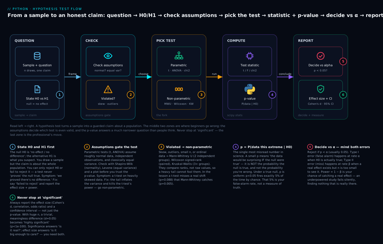
The six badges are the six places people go wrong, and this lesson is organised around them: stating H0 you can only reject-or-fail (1); letting assumptions pick the test (2); falling back to rank tests when they’re violated (3); reading the p-value as P(data | H0) and never P(H0 | data) (4); respecting both error types and power (5); and refusing to stop at “significant” without an effect size and interval (6).
You need three libraries beyond the Part 1 set. Always use a virtual environment — never pip install into the system Python:
python3 -m venv .venv
source .venv/bin/activate            # Windows: .venv\Scripts\activate
pip install numpy scipy pandas statsmodels scikit-learn
python -c "import scipy, statsmodels, sklearn; print(scipy.__version__, statsmodels.__version__, sklearn.__version__)"
# => 1.18.0 0.14.6 1.9.0   (any recent versions are fine)
scipy.stats gives you the tests; statsmodels gives you the rich statistical summaries (the ones with p-values and diagnostics, the R/Stata style); scikit-learn gives you the prediction-first machine-learning style. You’ll meet all three, and learn when each is the right tool. Every simulation below leans on vectorised NumPy — seeded default_rng generators and whole-array reductions, the reflexes from NumPy: Arrays, Broadcasting & Vectorization — and the regression data lives in pandas DataFrames, so those two lessons are the foundation this one builds on.
The hypothesis-testing framework
Everything starts by translating a vague question (“is the new flow better?”) into two mutually exclusive statements about the population.
The null hypothesis (H₀) is the boring default: no effect, no difference, nothing going on. “The two flows convert at the same rate.” “The coin is fair.” “Salary and tenure are uncorrelated.” The alternative hypothesis (H₁) is what you suspect: there is an effect. The entire procedure is built to give the null every benefit of the doubt and only reject it when the data would be genuinely surprising if it were true — the statistical version of “innocent until proven guilty.” H₀ is the presumption of innocence; the data is the evidence; the p-value measures how strained the innocence story has become.
Crucially, you never prove H₀. You either reject it (the evidence is strong enough) or fail to reject it (it isn’t). “We failed to reject the null” is not “we proved there’s no difference” — it might mean there’s no difference, or it might mean your sample was too small to see one. Conflating those two is the single most common error in applied science, and we’ll quantify it when we get to statistical power.
The test statistic and the p-value
A test statistic compresses your whole sample into one number that measures “how far is the data from what H₀ predicts, in units of noise?” For comparing two means it’s the t-statistic — roughly, the difference between the group means divided by the uncertainty in that difference. A t of 0 means the groups look identical; a t of 5 means they’re five noise-units apart, which almost never happens by chance.
The p-value converts that statistic into a probability, and its exact definition is the most important sentence in this lesson:
The p-value is the probability of observing data at least as extreme as yours, assuming the null hypothesis is true. It is
P(data this extreme | H₀).
Read the conditional carefully: the p-value is computed in a hypothetical world where H₀ holds. A small p-value (say 0.01) means “if there were truly no effect, data like this would show up only 1% of the time — so either something real is going on, or I got unlucky in a 1-in-100 way.” That is the entire content of the number. It is a statement about the data under an assumption, not a statement about the assumption.
Here is what the p-value is emphatically not, and each misreading has ended arguments (and reproducible science):
| Misinterpretation (all WRONG) | Why it’s wrong | What’s actually true |
|---|---|---|
| “p = 0.03 → 97% chance H₁ is true” | p is P(data | H₀), not P(H₁ | data) — you can’t flip a conditional |
p says nothing directly about the probability any hypothesis is true |
| “p = 0.03 → only 3% chance this is a fluke / false positive” | The false-positive rate depends on how often H₀ is true and on power, not on p alone | The long-run false-positive rate among “significant” findings can be far above 5% |
| “p = 0.51 → H₀ is true / no effect exists” | Failing to reject ≠ evidence for the null | Could be no effect, or an underpowered study missing a real one |
| “p just below 0.05 is solid; p = 0.06 is nothing” | 0.05 is an arbitrary convention, not a law of nature | A p of 0.049 and 0.051 are essentially identical evidence |
| “Smaller p → bigger / more important effect” | p conflates effect size with sample size | A tiny effect at huge n gives a microscopic p; report effect size separately |
Don’t take the definition on faith — simulate it. If the p-value really is “the chance of data this extreme when H₀ is true,” then when H₀ is true, p should be uniformly distributed on [0, 1], and p < 0.05 should happen exactly 5% of the time. Let’s draw two samples from the identical distribution 100,000 times (so the null is true by construction) and look at the p-values:
import numpy as np
from scipy import stats as sps

rng = np.random.default_rng(0)
N = 100_000
pvals = np.empty(N)
for i in range(N):
    x = rng.normal(0, 1, 30)
    y = rng.normal(0, 1, 30)      # SAME distribution -> H0 is TRUE
    pvals[i] = sps.ttest_ind(x, y).pvalue

print(f"P(p < 0.05) = {(pvals < 0.05).mean():.4f}")   # => P(p < 0.05) = 0.0493
print(f"P(p < 0.01) = {(pvals < 0.01).mean():.4f}")   # => P(p < 0.01) = 0.0100
print(f"P(p < 0.10) = {(pvals < 0.10).mean():.4f}")   # => P(p < 0.10) = 0.1009
print(f"mean p = {pvals.mean():.4f}")                 # => mean p = 0.4975  (uniform mean 0.5)
print("quartiles:", np.percentile(pvals, [25, 50, 75]).round(4))
# => quartiles: [0.2478 0.4952 0.7471]   (0.25/0.50/0.75 -> perfectly uniform)
There it is, mechanically. When nothing is going on, p < 0.05 fires 4.93% of the time, p < 0.01 fires 1.00% of the time, and the p-values spread uniformly from 0 to 1 (mean 0.4975, quartiles at 0.25/0.50/0.75). That 5% is not a measure of truth — it is the false-alarm rate you signed up for by choosing α = 0.05. Run twenty honest tests on effect-free data and you should expect one to come up “significant.” Hold that thought; it’s the seed of the multiple-comparisons disaster later.
α, and the two ways to be wrong
The threshold you compare the p-value against is α (alpha), the significance level — the false-positive rate you’re willing to tolerate. α = 0.05 is the near-universal (and arbitrary) convention; particle physicists use 0.0000003 (five sigma), and some fields are moving to 0.005. You choose α before seeing the data, and you reject H₀ when p < α.
Because you’re making a binary decision (reject / don’t) about an unknown reality (effect real / not), there are exactly two ways to be wrong:
| H₀ actually true (no effect) | H₀ actually false (real effect) | |
|---|---|---|
| You reject H₀ | ❌ Type I error (false positive) — prob = α | ✅ Correct — prob = power = 1 − β |
| You fail to reject H₀ | ✅ Correct — prob = 1 − α | ❌ Type II error (false negative) — prob = β |
A Type I error is a false alarm: you declare an effect that isn’t there. Its probability is exactly α — that’s what choosing α = 0.05 means. A Type II error is a miss: a real effect exists but your test doesn’t detect it, with probability β. Power (1 − β) is the probability of correctly detecting a real effect — the thing an underpowered study lacks. The mnemonic: Type I is convicting an innocent person; Type II is acquitting a guilty one; α is how often you’re willing to convict the innocent.
Power, and why underpowered studies fail silently
Power depends on three things you can control or estimate: the effect size (bigger effects are easier to see), the sample size n (more data, more power), and α (a stricter threshold catches fewer real effects too). Let’s measure power by brute force — draw two groups whose means genuinely differ by some amount, and count how often the t-test correctly rejects:
rng = np.random.default_rng(1)

def power_sim(delta, n, sd=1.0, alpha=0.05, trials=20000):
    """Fraction of trials where a real effect (delta) is detected."""
    rejections = 0
    for _ in range(trials):
        x = rng.normal(0,     sd, n)
        y = rng.normal(delta, sd, n)     # a REAL effect of size delta
        if sps.ttest_ind(x, y).pvalue < alpha:
            rejections += 1
    return rejections / trials

print(f"delta=0.0, n=30  -> {power_sim(0.0, 30):.4f}")   # => 0.0473  (H0 true: this is TYPE I = alpha)
print(f"delta=0.5, n=30  -> {power_sim(0.5, 30):.4f}")   # => 0.4729  (real effect, but coin-flip power!)
print(f"delta=0.5, n=100 -> {power_sim(0.5, 100):.4f}")  # => 0.9394  (4x the data -> 94% power)
print(f"delta=0.2, n=30  -> {power_sim(0.2, 30):.4f}")   # => 0.1183  (tiny effect: almost blind)
print(f"delta=0.2, n=200 -> {power_sim(0.2, 200):.4f}")  # => 0.5163
Read the second line and shudder: with a real, moderate effect (delta = 0.5) and n = 30 per group, the test detects it only 47% of the time. You’d miss a genuine effect on more than half your attempts — a coin flip dressed up as science. Quadruple the sample to n = 100 and power jumps to 94%. The first line confirms the framework: with no effect (delta = 0), the rejection rate is 4.73% — that’s the Type I rate, ≈ α, exactly as designed.
You don’t have to simulate power in practice; statsmodels computes it analytically and, more usefully, tells you the sample size you need:
from statsmodels.stats.power import TTestIndPower
analysis = TTestIndPower()

# power of a design (matches the simulation above):
print(analysis.power(effect_size=0.5, nobs1=30,  alpha=0.05))   # => 0.4779
print(analysis.power(effect_size=0.5, nobs1=100, alpha=0.05))   # => 0.9404

# the question you should actually ask BEFORE collecting data:
n = analysis.solve_power(effect_size=0.5, power=0.8, alpha=0.05)
print(f"n per group for 80% power at d=0.5: {n:.1f}")            # => 63.8  -> use 64
The analytic numbers (0.4779, 0.9404) match the simulation (0.4729, 0.9394) to within Monte-Carlo noise. And the last line is the professional habit: do a power analysis before you collect data, so you know you can actually detect the effect you care about. A study with 30% power that finds nothing has proven nothing — it was never able to see.
| Concept | Symbol | Plain meaning | Typical value |
|---|---|---|---|
| Significance level | α | Tolerated false-positive rate; reject if p < α |
0.05 |
| Type I error | α | False alarm — “effect” that isn’t real | 5% |
| Type II error | β | Miss — real effect not detected | 10–20% |
| Power | 1 − β | Chance of catching a real effect | aim for ≥ 0.80 |
| p-value | — | P(data this extreme | H₀) |
computed |
That α = 0.05 is a convention, not a constant of nature — the tolerable false-positive rate should scale with the stakes and the number of tests:
| Field / context | Conventional α | Why |
|---|---|---|
| Social science, business, A/B tests | 0.05 | The default convention (Fisher’s, ~1925) |
| Confirmatory medical trials | 0.01–0.05 | Higher stakes → stricter |
| Genome-wide association | 5×10⁻⁸ | Millions of simultaneous tests |
| Particle physics (“5-sigma”) | ~3×10⁻⁷ | Discovery-grade certainty |
| Exploratory / hypothesis-generating | 0.10 | Tolerate more false alarms to avoid missing leads |
And every test in this lesson works the same way under the hood: it maps its statistic onto a known reference distribution (the distribution that statistic would follow if H₀ were true) and reads off the tail area as the p-value. Knowing which distribution and how many degrees of freedom demystifies the output:
| Test | Statistic | Reference distribution under H₀ | Degrees of freedom |
|---|---|---|---|
| t-test | t | Student’s t | n−1 (one-sample); Welch approx (two-sample) |
| One-way ANOVA | F | F-distribution | (k−1, N−k) |
| Chi-square | χ² | Chi-square | k−1 (GOF); (r−1)(c−1) (independence) |
| Correlation test | t (from r) | Student’s t | n−2 |
| Mann-Whitney / Wilcoxon | U / W | normal approx (large n) | — (uses ranks) |
The t-tests: one-sample, two-sample, paired
The t-test compares means, and it comes in three flavours matched to three questions. We’ll use a concrete scenario throughout: two checkout backends, A and B, and their per-session response times in milliseconds. Build the data once with a seed so your numbers match:
import numpy as np
from scipy import stats as sps

rng = np.random.default_rng(42)
a = rng.normal(210, 18, size=60)     # backend A response times (ms)
b = rng.normal(200, 18, size=60)     # backend B response times (ms)

print(f"A: n={a.size}  mean={a.mean():.3f}  sd={a.std(ddof=1):.3f}")  # => A: n=60 mean=211.175 sd=14.142
print(f"B: n={b.size}  mean={b.mean():.3f}  sd={b.std(ddof=1):.3f}")  # => B: n=60 mean=196.650 sd=13.863
print(f"observed difference (A - B) = {a.mean() - b.mean():.3f} ms")  # => 14.525 ms
One-sample t-test — is the mean different from a target?
The one-sample t-test asks whether a single group’s mean differs from a fixed reference value. Suppose your SLA target is 205 ms — is backend A significantly above it?
res = sps.ttest_1samp(a, popmean=205)
print(f"t = {res.statistic:.4f}   p = {res.pvalue:.4f}")   # => t = 3.3824   p = 0.0013
print("95% CI of A's mean:", res.confidence_interval(0.95))
# => ConfidenceInterval(low=207.522, high=214.828)
p = 0.0013 < 0.05: A’s mean (211.2 ms) is significantly above the 205 ms target. The 95% confidence interval [207.5, 214.8] doesn’t contain 205, which is the same conclusion viewed as a range — a duality we’ll formalise shortly.
Two-sample t-test — do two groups differ?
The two-sample (independent) t-test is the workhorse: do A and B have different mean response times? H₀ is “same mean.” But before you trust it, check the assumptions — this is badge 2 on the diagram, and skipping it is how the t-test lies.
# Assumption 1: each group is roughly normal (Shapiro-Wilk; H0 = normal)
print("Shapiro A:", sps.shapiro(a).pvalue)    # => 0.9476  (p > 0.05 -> can't reject normal: OK)
print("Shapiro B:", sps.shapiro(b).pvalue)    # => 0.4072  (OK)

# Assumption 2: equal variances? (Levene; H0 = equal variance)
print("Levene:", sps.levene(a, b).pvalue)     # => 0.8722  (p > 0.05 -> equal variance: OK)
Both Shapiro p-values are large (0.95, 0.41), so we can’t reject normality; Levene’s p is 0.87, so variances look equal. Assumptions met — the t-test is valid here. Now run it:
# Welch's t-test (does NOT assume equal variance) -- the safer default
welch = sps.ttest_ind(a, b, equal_var=False)
print(f"Welch:   t = {welch.statistic:.4f}   p = {welch.pvalue:.3e}")
# => Welch:   t = 5.6813   p = 9.804e-08

# Student's t-test (assumes equal variance) -- only when Levene says it's safe
student = sps.ttest_ind(a, b, equal_var=True)
print(f"Student: t = {student.statistic:.4f}   p = {student.pvalue:.3e}")
# => Student: t = 5.6813   p = 9.798e-08

# 95% confidence interval on the DIFFERENCE of means:
print("95% CI (A - B):", sps.ttest_ind(a, b).confidence_interval(0.95))
# => ConfidenceInterval(low=9.462, high=19.588)
p ≈ 1e-7: the difference is real, not noise. The 95% CI on the difference is [9.5, 19.6] ms and doesn’t include 0 — consistent with “significant.” Note that Welch and Student give nearly identical answers here because the variances happen to be equal; when they’re not, only Welch is trustworthy.
⚠️ Prefer equal_var=False (Welch’s t-test) as your default. It doesn’t assume equal variances and costs almost nothing in power when they are equal. scipy’s default is equal_var=True (Student’s), which is the more fragile choice — so override it. This is the opposite of most people’s habit.
One-tailed vs two-tailed
By default the t-test is two-tailed: H₁ is “the means differ” (in either direction). If you have a directional hypothesis decided in advance — “A is slower than B” — you can run a one-tailed test, which puts all of α in one tail and roughly halves the p-value:
one_sided = sps.ttest_ind(a, b, equal_var=False, alternative='greater')  # H1: mean(A) > mean(B)
print(f"one-tailed p = {one_sided.pvalue:.3e}")   # => 4.902e-08  (half the two-tailed p)
⚠️ Never pick the tail after seeing the data. Deciding the direction because the data already leans that way secretly doubles your false-positive rate — it’s a form of p-hacking. Use one-tailed tests only when the direction was fixed by the hypothesis before collection, and when the other direction would be genuinely uninteresting.
Paired t-test — before-and-after on the same units
When the two measurements are on the same subjects — the same servers before and after an optimisation, the same users on two designs — they’re paired, and using an independent test throws away the pairing and most of your power. The paired t-test analyses the per-unit differences:
rng = np.random.default_rng(11)
before = rng.normal(150, 25, 40)        # response time per server, before tuning
improvement = rng.normal(8, 10, 40)     # each server improves by ~8ms (correlated with itself)
after = before - improvement

paired = sps.ttest_rel(before, after)
print(f"paired:   t = {paired.statistic:.4f}   p = {paired.pvalue:.3e}")
# => paired:   t = 6.5810   p = 8.099e-08   (clearly significant)

# The WRONG way -- treat them as independent, losing the pairing:
wrong = sps.ttest_ind(before, after)
print(f"unpaired: t = {wrong.statistic:.4f}   p = {wrong.pvalue:.4f}")
# => unpaired: t = 1.9124   p = 0.0595   (MISSES it -- p > 0.05!)
Same data, opposite conclusions. The paired test sees the consistent per-server improvement and reports p = 8e-8; the unpaired test, blind to the pairing, drowns that signal in the large between-server variance and reports p = 0.0595 — not significant. Pairing, when it exists, is free statistical power. Throwing it away is a Type II error waiting to happen.
| Question | Test | scipy call | H₀ |
|---|---|---|---|
| One group’s mean vs a fixed target | One-sample t | ttest_1samp(x, target) |
mean = target |
| Two independent groups’ means | Two-sample (Welch) t | ttest_ind(x, y, equal_var=False) |
mean₁ = mean₂ |
| Same units measured twice | Paired t | ttest_rel(before, after) |
mean difference = 0 |
| Directional, pre-registered | One-tailed | ttest_*(..., alternative='greater'/'less') |
one-sided |
When assumptions break: non-parametric fallbacks
The t-test, ANOVA, and friends are parametric — they assume the data follows (roughly) a specific shape, almost always the normal distribution, plus independence and often equal variance. When those assumptions hold, they’re the most powerful tools available. When they don’t, the p-value they hand you is fiction, and the software won’t tell you.
The three assumptions, how to check them, and why each matters:
| Assumption | What it means | Check with | If violated |
|---|---|---|---|
| Normality | Each group ≈ normally distributed | sps.shapiro(x), Q-Q plot, sps.skew |
Non-parametric test, or transform (log) |
| Equal variance | Groups have similar spread (homoscedasticity) | sps.levene(x, y) |
Welch’s t (auto-handles it); Welch ANOVA |
| Independence | Observations don’t influence each other | Study design; durbin_watson for series |
Paired/repeated-measures test; mixed models |
You don’t eyeball these — there’s a formal test for each, and scipy has them all. The one rule to remember: for these assumption checks, H₀ is “the assumption holds,” so you want a large p-value (failing to reject = assumption OK):
| Check | Test | H₀ | Call |
|---|---|---|---|
| Normality (general) | Shapiro-Wilk | data is normal | sps.shapiro(x) |
| Normality (large n) | D’Agostino K² | data is normal | sps.normaltest(x) |
| Normality (vs a named dist) | Anderson-Darling | data follows the dist | sps.anderson(x) |
| Equal variance (robust) | Levene | variances equal | sps.levene(x, y) |
| Equal variance (if normal) | Bartlett | variances equal | sps.bartlett(x, y) |
| No autocorrelation | Durbin-Watson | residuals independent | durbin_watson(resid) |
Normality matters least for large samples — the Central Limit Theorem from Part 1 rescues the t-test on big n even from non-normal data, because it works on the sample mean, which becomes normal regardless. But on small, skewed samples the t-test’s power collapses, because the mean and variance it depends on are both hijacked by the tail. That’s exactly when you reach for a non-parametric test — one that works on ranks instead of raw values, so a heavy tail can’t fool it.
Here is the killer example. Two skewed groups (think API latencies — a log-normal body with a long tail), n = 45 each, where B is genuinely shifted higher:
rng = np.random.default_rng(50)
g1 = rng.lognormal(3.0,  0.7, 45)     # skewed group 1
g2 = rng.lognormal(3.25, 0.7, 45)     # skewed group 2, shifted up

print(f"g1: mean={g1.mean():.2f}  median={np.median(g1):.2f}  skew={sps.skew(g1):.2f}")
# => g1: mean=24.68  median=17.49  skew=3.15   (mean >> median: violently right-skewed)
print(f"g2: mean={g2.mean():.2f}  median={np.median(g2):.2f}  skew={sps.skew(g2):.2f}")
# => g2: mean=33.82  median=28.17  skew=1.69

# Assumption check: are they normal?
print(f"Shapiro g1 p = {sps.shapiro(g1).pvalue:.1e}")   # => 1.8e-09  (NOT normal -- reject hard)
print(f"Shapiro g2 p = {sps.shapiro(g2).pvalue:.1e}")   # => 7.3e-06  (NOT normal)
The Shapiro p-values are microscopic (1.8e-09, 7.3e-06): normality is decisively violated. The t-test’s assumptions don’t hold. But watch what happens if you run it anyway versus the correct rank-based Mann-Whitney U test:
t_test = sps.ttest_ind(g1, g2, equal_var=False)
mwu    = sps.mannwhitneyu(g1, g2, alternative='two-sided')

print(f"t-test:        t = {t_test.statistic:.4f}   p = {t_test.pvalue:.4f}")
# => t-test:        t = -1.7259   p = 0.0879   <- MISSES it (p > 0.05: "no difference")
print(f"Mann-Whitney:  U = {mwu.statistic:.1f}    p = {mwu.pvalue:.4f}")
# => Mann-Whitney:  U = 664.0    p = 0.0050   <- CATCHES it (clearly significant)
print(f"medians: {np.median(g1):.1f} vs {np.median(g2):.1f} ms")   # => 17.5 vs 28.2 ms
The t-test says p = 0.088, “no significant difference.” The Mann-Whitney says p = 0.005, a clear difference — and the medians (17.5 vs 28.2 ms) confirm the shift is real and large. The t-test failed because the fat tails inflated both group variances, blowing up the denominator of the t-statistic and destroying its power. The rank-based test never looks at the raw values — only their order — so the tail can’t distort it. When your assumption check fails, the non-parametric test isn’t a weaker consolation prize; here it’s the only one telling the truth.
⚠️ There’s a second valid fix: transform, then test. Log-transforming right-skewed data often restores normality, after which a t-test on the logs is fair (sps.ttest_ind(np.log(g1), np.log(g2)).pvalue = 0.0076 — it agrees with Mann-Whitney). Choose transformation when you want to keep the parametric machinery (and can defend the transform); choose the rank test when you just want a robust answer.
Every parametric test has a rank-based twin for exactly this situation:
| Parametric test (assumes normal) | Non-parametric fallback | scipy call | Compares |
|---|---|---|---|
| Two-sample t-test | Mann-Whitney U | sps.mannwhitneyu(x, y) |
Two independent groups (ranks) |
| Paired t-test | Wilcoxon signed-rank | sps.wilcoxon(before, after) |
Paired differences (ranks) |
| One-way ANOVA | Kruskal-Wallis H | sps.kruskal(a, b, c) |
3+ independent groups (ranks) |
| Pearson correlation | Spearman / Kendall | sps.spearmanr(x, y) |
Monotonic association (ranks) |
The trade-off: non-parametric tests make fewer assumptions and are robust to outliers and skew, but when the data is normal they’re slightly less powerful (they ignore the magnitude information in the values). The rule of thumb: check normality; if it clearly fails on a smallish sample, use the rank test. For the paired case, the Wilcoxon signed-rank confirms our earlier paired result without assuming normality (sps.wilcoxon(before, after).pvalue = 3.14e-07).
Comparing many groups: ANOVA and chi-square
One-way ANOVA — three or more means at once
Got three groups? Don’t run three t-tests — that inflates your false-positive rate (the multiple-comparisons problem, next section). One-way ANOVA (Analysis of Variance) tests them all at once. H₀ is “all group means are equal”; H₁ is “at least one differs.” Its F-statistic is the ratio of between-group variance to within-group variance — if the groups are spread apart relative to their internal scatter, F is large and p is small.
rng = np.random.default_rng(5)
region1 = rng.normal(100, 12, 50)     # latency by data-centre region (ms)
region2 = rng.normal(104, 12, 50)
region3 = rng.normal(110, 12, 50)

print("Levene (equal var?):", sps.levene(region1, region2, region3).pvalue)  # => 0.9040 (OK)
F, p = sps.f_oneway(region1, region2, region3)
print(f"ANOVA: F = {F:.4f}   p = {p:.3e}")   # => ANOVA: F = 27.7189   p = 6.101e-11
p = 6e-11: at least one region differs. But ANOVA is an omnibus test — it tells you that the groups differ, not which ones. For that you need a post-hoc test that compares every pair while controlling the overall error rate. Tukey’s HSD is the standard:
from statsmodels.stats.multicomp import pairwise_tukeyhsd

values = np.concatenate([region1, region2, region3])
labels = ['r1']*50 + ['r2']*50 + ['r3']*50
print(pairwise_tukeyhsd(values, labels, alpha=0.05))
 Multiple Comparison of Means - Tukey HSD, FWER=0.05
====================================================
group1 group2 meandiff p-adj   lower   upper  reject
----------------------------------------------------
    r1     r2   6.4137 0.0097  1.2987 11.5286   True
    r1     r3  15.9815    0.0 10.8666 21.0964   True
    r2     r3   9.5678 0.0001  4.4529 14.6828   True
----------------------------------------------------
Every pair differs significantly (all reject = True), and Tukey gives you the effect (meandiff) and a confidence interval for each pairwise gap, with the p-values already adjusted for making three comparisons. If the normality assumption were violated, the non-parametric twin is Kruskal-Wallis (sps.kruskal(region1, region2, region3).pvalue = 2.34e-09 here — same conclusion).
Chi-square — for counts and categories
The t-test and ANOVA compare means of numeric data. When your data is categorical — counts in buckets — you need the chi-square (χ²) test, which compares observed counts to expected counts. It comes in two forms.
Goodness-of-fit asks: does one categorical variable match an expected distribution? Is a six-sided die fair after 600 rolls?
observed = np.array([90, 105, 98, 110, 92, 105])     # counts for faces 1..6
expected = np.full(6, observed.sum() / 6)            # fair die -> 100 each
chi2, p = sps.chisquare(observed, expected)
print(f"goodness-of-fit: chi2 = {chi2:.4f}   p = {p:.4f}")   # => chi2 = 3.1800   p = 0.6723
p = 0.67: we fail to reject — no evidence the die is unfair. The deviations from 100 are ordinary sampling noise. (Note: failing to reject is not proof the die is perfectly fair — see the framework section.)
Test of independence asks: are two categorical variables related? Do subscription tier and churn move together?
# rows = plan (Free/Pro/Enterprise), cols = [stayed, churned]
table = np.array([[200, 50],      # Free
                  [220, 30],      # Pro
                  [260, 15]])     # Enterprise
chi2, p, dof, expected = sps.chi2_contingency(table)
print(f"independence: chi2 = {chi2:.4f}   p = {p:.3e}   dof = {dof}")
# => independence: chi2 = 25.7824   p = 2.520e-06   dof = 2
print("expected counts under independence:\n", np.round(expected, 2))
# => [[219.35  30.65]
#     [219.35  30.65]
#     [241.29  33.71]]

# Effect size for chi-square: Cramér's V (0 = none, 1 = perfect)
n_total, k = table.sum(), min(table.shape) - 1
cramers_v = np.sqrt(chi2 / (n_total * k))
print(f"Cramér's V = {cramers_v:.4f}")   # => Cramér's V = 0.1824  (a small-to-moderate effect)
p = 2.5e-6: churn and plan are not independent — higher tiers churn less (Free’s observed 50 churns exceed the 30.65 expected under independence). But note the Cramér’s V of 0.18: the association is statistically rock-solid yet only small-to-moderate in strength. That gap between “definitely real” and “only moderately strong” is the theme of the next section, and the whole reason effect size exists.
⚠️ Chi-square needs adequate expected counts. The common rule: every expected cell should be ≥ 5 (some allow a few at ≥ 1). With sparse tables, scipy applies Yates’ continuity correction for 2×2 tables by default, or you switch to Fisher’s exact test (sps.fisher_exact) for small 2×2 counts.
You’ve now seen every core test. Here is the whole decision, condensed into the one lookup table worth bookmarking — read the question in the left column, then pick the valid test based on whether the assumptions hold:
| Your data & question | Assumptions OK → | Assumptions violated → |
|---|---|---|
| One group’s mean vs a target | One-sample t-test | Wilcoxon signed-rank (vs median) |
| Two independent groups | Welch’s t-test | Mann-Whitney U |
| Two paired measurements | Paired t-test | Wilcoxon signed-rank |
| 3+ independent groups | One-way ANOVA + Tukey | Kruskal-Wallis + Dunn |
| Two categorical variables | Chi-square independence | Fisher’s exact (small n) |
| One categorical vs expected | Chi-square goodness-of-fit | (exact multinomial) |
| Association of two numerics | Pearson correlation | Spearman / Kendall |
| Predict a numeric outcome | OLS regression | robust SEs / GLM |
| Predict a binary outcome | Logistic regression | — |
Effect size and confidence intervals
A p-value answers exactly one question: “is this effect distinguishable from zero?” It says nothing about how big the effect is. Those are different questions, and conflating them is the mistake in that opening rocket-emoji story. Effect size answers the second question, in units that don’t depend on sample size.
Cohen’s d — the standardised difference
For a difference in means, the standard effect size is Cohen’s d: the difference between the means, divided by the pooled standard deviation. It’s a z-score for the gap between two groups — how many standard deviations apart their means are, independent of n.
def cohens_d(x, y):
    nx, ny = len(x), len(y)
    pooled_sd = np.sqrt(((nx-1)*x.var(ddof=1) + (ny-1)*y.var(ddof=1)) / (nx+ny-2))
    return (x.mean() - y.mean()) / pooled_sd

rng = np.random.default_rng(42)
a = rng.normal(210, 18, 60)
b = rng.normal(200, 18, 60)
print(f"Cohen's d = {cohens_d(a, b):.4f}")   # => Cohen's d = 1.0373  (a LARGE effect)
The checkout backends differ by d = 1.04 — the mean response times are more than a full standard deviation apart. That’s a large effect (users would feel it), and it’s what makes the tiny p-value meaningful. The conventional (rough) benchmarks:
| Cohen’s d | Interpretation | Rough overlap of the two groups |
|---|---|---|
| 0.2 | Small | groups heavily overlap |
| 0.5 | Medium | visible to the naked eye |
| 0.8 | Large | clearly separated |
| ≥ 1.0 | Very large | barely overlapping |
Cohen’s d is for a difference of means; every other test has its own effect-size measure, and reporting the right one is what turns “significant” into “significant and this big”:
| Test / situation | Effect size | Small / Medium / Large | How to get it |
|---|---|---|---|
| Two means | Cohen’s d | 0.2 / 0.5 / 0.8 | pooled-sd formula (above) |
| Correlation | Pearson r | 0.1 / 0.3 / 0.5 | sps.pearsonr |
| ANOVA | eta-squared η² | 0.01 / 0.06 / 0.14 | SS_between / SS_total |
| Chi-square | Cramér’s V | 0.1 / 0.3 / 0.5 | √(χ² / (n·k)) |
| Mann-Whitney | rank-biserial r | 0.1 / 0.3 / 0.5 | 1 − 2U/(n₁n₂) |
| Logistic regression | odds ratio | 1.0 = no effect | exp(coef) |
The tyranny of large n — significance ≠ importance
Here is the demonstration that should change how you read every “significant” result. Take a truly trivial effect — two groups whose means differ by just 0.05 standard deviations, an effect so small it’s meaningless in any real context — and watch what sample size does to the p-value. We draw one big pair of samples and evaluate growing prefixes of it, so it’s literally the same trivial effect measured with more and more data:
rng = np.random.default_rng(7)
big = 2_000_000
xall = rng.normal(0.00, 1.0, big)
yall = rng.normal(0.05, 1.0, big)     # TRUE effect: d = 0.05  (utterly trivial)

for n in [40, 400, 4000, 40000, 400000, 2000000]:
    x, y = xall[:n], yall[:n]
    p = sps.ttest_ind(x, y).pvalue
    d = abs(cohens_d(x, y))
    verdict = "SIGNIFICANT" if p < 0.05 else "not sig"
    print(f"n={n:>8}:  |d|={d:.3f}   p={p:.2e}   {verdict}")
n=      40:  |d|=0.379   p=9.40e-02   not sig
n=     400:  |d|=0.146   p=3.90e-02   SIGNIFICANT
n=    4000:  |d|=0.085   p=1.56e-04   SIGNIFICANT
n=   40000:  |d|=0.071   p=9.05e-24   SIGNIFICANT
n=  400000:  |d|=0.051   p=2.40e-114  SIGNIFICANT
n= 2000000:  |d|=0.051   p=0.00e+00   SIGNIFICANT
Read down the p-value column: the identical, meaningless effect goes from “not significant” to p ≈ 10⁻¹¹⁴ purely because n grew. With two million points, a difference of one-twentieth of a standard deviation has a p-value of literally zero — and it is still a difference nobody would ever care about. Meanwhile the effect size |d| correctly converges to the true 0.05 and stays trivially small the whole way down. (The noisy |d| = 0.379 at n = 40 is a bonus lesson: small samples overestimate effect sizes wildly — the “winner’s curse” behind many un-replicable headline findings.)
⚠️ This is why “statistically significant” from a big-data pipeline means almost nothing on its own. At Google/Meta/Amazon scale, everything is significant — every button colour, every pixel. The only question worth asking is the effect size: is the difference big enough to matter? Always report the effect size next to the p-value. A result is worth acting on only when it’s both significant (probably real) and large enough (worth the cost).
Confidence intervals and what “95%” actually means
A confidence interval (CI) is the effect-size answer with its uncertainty attached: instead of a single p-value verdict, it gives a range of plausible values for the true effect. The 95% CI on the A−B difference was [9.5, 19.6] ms — the true difference is plausibly anywhere in there, and because it excludes 0, the result is “significant” at α = 0.05. CIs and two-sided tests are dual: the 95% CI contains exactly the null values you’d fail to reject at α = 0.05.
But the interpretation is subtle, and almost everyone gets it backwards. A 95% CI does not mean “there’s a 95% probability the true value is in this interval.” The true value is fixed; your interval either contains it or doesn’t. The 95% is a property of the procedure: 95% of the intervals you’d construct this way, over many samples, contain the true value. Prove it by building 10,000 intervals from a known population (true mean = 100) and counting hits:
rng = np.random.default_rng(2024)
true_mu, hits, trials = 100.0, 0, 10_000
for _ in range(trials):
    sample = rng.normal(true_mu, 15, 40)
    m, se = sample.mean(), sample.std(ddof=1) / np.sqrt(40)
    tcrit = sps.t.ppf(0.975, df=39)
    lo, hi = m - tcrit*se, m + tcrit*se
    hits += (lo <= true_mu <= hi)
print(f"95% CIs that contained the true mean: {hits/trials:.4f}")   # => 0.9483
94.83% of the intervals caught the true mean — bang on the promised 95% (a 90% CI catches it 89.8% of the time, a 99% CI 99.0%). That is what “95% confident” means: not a probability about your one interval, but a hit-rate of the method. Any single interval you compute has already either caught the true value or missed it; you just don’t know which.
The interpretations, sorted into the ones that are right and the ones everyone reaches for:
| Statement about a 95% CI | Correct? | Why |
|---|---|---|
| “95% of intervals built this way contain the true value” | ✅ | The procedure’s long-run hit rate — verified above |
| “95% probability the true value is in this interval” | ❌ | The value is fixed; this interval already hit or missed |
| “95% of the data falls inside the interval” | ❌ | It’s about the parameter, not the spread of data points |
| “A wider interval means more confident” | ❌ | Higher confidence widens it, but more data narrows it |
| “It excludes 0, so the effect is significant at α=0.05” | ✅ | CI–test duality (two-sided) |
For a robust statistic like the median, or any quantity without a neat formula, you get a CI by bootstrapping — resampling your data with replacement thousands of times and reading off the percentiles:
rng = np.random.default_rng(50)
g1 = rng.lognormal(3.0, 0.7, 45)
boot_medians = np.array([np.median(rng.choice(g1, 45, replace=True)) for _ in range(10_000)])
print(f"median = {np.median(g1):.2f}   bootstrap 95% CI = "
      f"[{np.percentile(boot_medians, 2.5):.2f}, {np.percentile(boot_medians, 97.5):.2f}]")
# => median = 17.49   bootstrap 95% CI = [13.74, 23.84]
The bootstrap is the Swiss-army knife of inference: no formula, no normality assumption, just resampling. It gives an honest interval for the median of skewed data where no textbook formula applies.
The multiple-comparisons problem
Recall the p-value simulation: under a true null, p < 0.05 happens 5% of the time by chance. Now flip that around. If you run 20 independent tests where nothing is real, how many “significant” results should you expect? About one. Run 100, expect five. This is the multiple-comparisons problem, and it silently manufactures false discoveries everywhere from A/B testing dashboards to genomics.
Watch it happen — 20 tests, every one on pure noise (H₀ true everywhere):
rng = np.random.default_rng(8)
pvals = np.array([sps.ttest_ind(rng.normal(0,1,50), rng.normal(0,1,50)).pvalue
                  for _ in range(20)])
print(np.round(pvals, 4))
# => [0.1421 0.1098 0.9897 0.0924 0.8895 0.0055 0.7039 0.2955 0.374  0.0152
#     0.6521 0.4893 0.067  0.4698 0.7737 0.8275 0.1803 0.839  0.6961 0.5422]
print(f"'significant' at 0.05: {(pvals < 0.05).sum()}   min p = {pvals.min():.4f}")
# => 'significant' at 0.05: 2   min p = 0.0055
print(f"P(at least one false positive in 20) = {1 - 0.95**20:.4f}")   # => 0.6415
Two of the twenty came up “significant,” one at p = 0.0055 that looks impressively strong — and every single one is a false positive, because we built the data with no effect at all. The probability of getting at least one false alarm across 20 null tests is 1 − 0.95²⁰ = 64%. So if you run a dashboard with 20 metrics and celebrate whichever crosses 0.05, you are celebrating noise almost two times out of three. This is the mechanism behind p-hacking: test many things (or many subgroups, or many time windows) and report only the ones that “worked.”
The fix is to correct for the number of comparisons. The strictest is the Bonferroni correction — divide α by the number of tests m (here 0.05/20 = 0.0025). The Benjamini-Hochberg procedure is less conservative, controlling the false discovery rate instead:
from statsmodels.stats.multitest import multipletests

bonf = multipletests(pvals, alpha=0.05, method='bonferroni')[0]
bh   = multipletests(pvals, alpha=0.05, method='fdr_bh')[0]
print(f"Bonferroni (threshold {0.05/20:.4f}): {bonf.sum()} survive")   # => 0 survive
print(f"Benjamini-Hochberg:                  {bh.sum()} survive")      # => 0 survive
Both corrections wipe out all the false positives: the “impressive” p = 0.0055 doesn’t clear the Bonferroni bar of 0.0025, so nothing is declared significant — which is correct, since nothing was real.
| Approach | Threshold logic | Controls | When to use |
|---|---|---|---|
| No correction | each test at α | nothing (inflates errors) | a single pre-planned test |
| Bonferroni | α / m | family-wise error (any false positive) | few tests, want to be strict |
| Benjamini-Hochberg | ramped by rank | false discovery rate (proportion of false positives) | many tests (genomics, A/B suites) |
⚠️ The honest defence against p-hacking is to decide your analysis before you see the data. Pre-register the hypothesis, the test, and the sample size. Report all the comparisons you ran, not just the survivors. “We tested 40 subgroups and one hit p = 0.04” is not a finding; it’s an expected accident. This discipline is the practical core of the replication crisis we close on.
Correlation: Pearson, Spearman, Kendall
Correlation measures how two variables move together, on a scale from −1 (perfect opposite) through 0 (no linear/monotonic relationship) to +1 (perfect together). There are three common coefficients, and choosing the wrong one hides real relationships.
Pearson’s r measures linear association — how well the points hug a straight line. Spearman’s ρ correlates the ranks, so it captures any monotonic relationship (consistently up or down, even if curved) and is robust to outliers. Kendall’s τ also works on ranks but measures the fraction of concordant vs discordant pairs — more interpretable and more robust on small or tied data. Watch them disagree on data with a real but curved relationship:
rng = np.random.default_rng(3)
x = rng.uniform(1, 100, 300)
y = np.log(x) + rng.normal(0, 0.15, 300)     # real relationship, but CURVED (logarithmic)

print(f"Pearson  r   = {sps.pearsonr(x, y).statistic:.4f}")    # => 0.8817
print(f"Spearman rho = {sps.spearmanr(x, y).statistic:.4f}")   # => 0.9483
print(f"Kendall  tau = {sps.kendalltau(x, y).statistic:.4f}")  # => 0.8182
Spearman (0.95) sees the relationship more clearly than Pearson (0.88) because it doesn’t demand a straight line, only a consistent direction. Push to a perfectly monotonic curve and the gap becomes stark:
xm = np.arange(1, 101.0); ym = xm**3        # perfect monotonic curve
print(f"y=x^3:  Pearson={sps.pearsonr(xm,ym).statistic:.4f}  "
      f"Spearman={sps.spearmanr(xm,ym).statistic:.4f}")
# => y=x^3:  Pearson=0.9176  Spearman=1.0000
Spearman reports a perfect 1.0 (the relationship is perfectly monotonic); Pearson only 0.92 because the curve isn’t a straight line. If you’d screened features by Pearson and dropped anything below 0.95, you’d have thrown away a perfectly predictive variable.
And the trap that catches everyone — a non-monotonic relationship (a U-shape) where the variables are perfectly related but both coefficients read ≈ 0:
xp = np.linspace(-10, 10, 201); yp = xp**2   # y fully determined by x, but U-shaped
print(f"y=x^2:  Pearson={sps.pearsonr(xp,yp).statistic:.4f}  "
      f"Spearman={sps.spearmanr(xp,yp).statistic:.4f}")
# => y=x^2:  Pearson=0.0000  Spearman=0.0047
y is a deterministic function of x, yet both correlations are essentially zero, because the up-half cancels the down-half. A correlation near zero means “no monotonic relationship,” not “no relationship.” The only defence is to plot your data — which brings us to the most famous demonstration in statistics.
| Coefficient | Captures | Robust to outliers? | Use when |
|---|---|---|---|
Pearson r |
Linear association | No | Both variables ≈ normal, relationship is straight-line |
Spearman ρ |
Monotonic (any consistent direction) | Yes | Curved-but-monotonic, ordinal data, outliers |
Kendall τ |
Concordant/discordant pairs | Yes (most) | Small samples, many ties, want interpretability |
And a rough dictionary for turning a coefficient into words (context always matters — an r of 0.3 is huge in social science, trivial in physics):
| |r| or |ρ| | Strength (rough) |
|---|---|
| 0.0 – 0.1 | negligible |
| 0.1 – 0.3 | weak |
| 0.3 – 0.5 | moderate |
| 0.5 – 0.7 | strong |
| 0.7 – 0.9 | very strong |
| 0.9 – 1.0 | near-perfect |
Anscombe’s quartet — why you must plot
In 1973 the statistician Francis Anscombe built four tiny datasets that are nearly identical in every summary statistic — same means, same variances, same correlation, same regression line — yet look completely different when plotted. Compute the summaries and see for yourself:
import numpy as np
from scipy import stats as sps

x    = np.array([10, 8, 13, 9, 11, 14, 6, 4, 12, 7, 5], float)
y1   = np.array([8.04,6.95,7.58,8.81,8.33,9.96,7.24,4.26,10.84,4.82,5.68])
y2   = np.array([9.14,8.14,8.74,8.77,9.26,8.10,6.13,3.10,9.13,7.26,4.74])
y3   = np.array([7.46,6.77,12.74,7.11,7.81,8.84,6.08,5.39,8.15,6.42,5.73])
x4   = np.array([8,8,8,8,8,8,8,19,8,8,8], float)
y4   = np.array([6.58,5.76,7.71,8.84,8.47,7.04,5.25,12.50,5.56,7.91,6.89])

for name, xx, yy in [("I", x, y1), ("II", x, y2), ("III", x, y3), ("IV", x4, y4)]:
    r = sps.pearsonr(xx, yy).statistic
    slope, intercept, *_ = sps.linregress(xx, yy)
    print(f"Set {name:>3}: mean_y={yy.mean():.2f}  var_y={yy.var(ddof=1):.2f}  "
          f"r={r:.3f}  line: y={slope:.2f}x+{intercept:.2f}")
Set   I: mean_y=7.50  var_y=4.13  r=0.816  line: y=0.50x+3.00
Set  II: mean_y=7.50  var_y=4.13  r=0.816  line: y=0.50x+3.00
Set III: mean_y=7.50  var_y=4.12  r=0.816  line: y=0.50x+3.00
Set  IV: mean_y=7.50  var_y=4.12  r=0.817  line: y=0.50x+3.00
Four datasets, one set of numbers. Same mean (7.50), same variance (4.12), same correlation (r = 0.816), same fitted line (y = 0.50x + 3.00). Yet: Set I is a genuine noisy linear relationship (the summary is honest); Set II is a smooth curve (a parabola — linear correlation is the wrong model entirely); Set III is a perfect line ruined by a single outlier dragging the fit off; Set IV is a vertical stack of identical x-values plus one far-off point that single-handedly invents the entire correlation. If you’d trusted the r of 0.816 without plotting, you’d have drawn four confidently wrong conclusions. Anscombe’s quartet is the reason “always visualise your data” is not a platitude — see Matplotlib: Plotting Basics for the how.
| Set | What it actually is | What the identical summary hides |
|---|---|---|
| I | A genuine noisy linear relationship | Nothing — here the statistics are honest |
| II | A smooth curve (parabola) | Linearity is wrong; the model doesn’t fit the shape |
| III | A perfect line + one outlier | The outlier drags the fitted slope off the true line |
| IV | A vertical stack + one far point | A single high-leverage point invents the whole correlation |
⚠️ Correlation is not causation — the rule to tattoo inside your eyelids. A strong r between two variables means they move together; it does not mean one causes the other. Ice-cream sales correlate with drowning deaths (summer causes both — a confounder). Two independent random walks can correlate at 0.9 by chance (spurious correlation). Reverse causation is always possible (does exercise cause health, or do healthy people exercise?). Correlation is a hint to investigate, never a conclusion. Establishing causation needs a randomised experiment or careful causal inference — not a high coefficient.
Linear regression with OLS
Correlation says whether two variables move together; regression models how — it fits an equation you can interpret and predict from. Ordinary Least Squares (OLS) finds the line (or hyperplane) minimising the sum of squared vertical distances from the points. We’ll model house prices (₹ lakh) from size (sqft) and age (years), with statsmodels for the rich statistical summary:
import numpy as np, pandas as pd
import statsmodels.api as sm

rng = np.random.default_rng(21)
n = 200
size = rng.uniform(500, 3000, n)
age  = rng.uniform(0, 40, n)
# TRUE model: price = 50 + 0.10*size - 1.5*age + noise
price = 50 + 0.10*size - 1.5*age + rng.normal(0, 20, n)
df = pd.DataFrame({"price": price, "size": size, "age": age})

# SIMPLE regression: price ~ size  (add_constant gives us the intercept term)
X1 = sm.add_constant(df["size"])
m1 = sm.OLS(df["price"], X1).fit()
print(f"intercept = {m1.params.iloc[0]:.3f}   size coef = {m1.params.iloc[1]:.5f}")
# => intercept = 22.800   size coef = 0.09968
print(f"R2 = {m1.rsquared:.4f}   adj R2 = {m1.rsquared_adj:.4f}")   # => R2 = 0.8907  adj R2 = 0.8901
The coefficient on size is 0.0997, meaning each extra square foot adds ≈ ₹0.10 lakh to the predicted price — and it recovered the true 0.10 we built in. Now add age for a multiple regression and read the full summary, the document you’ll meet everywhere:
X2 = sm.add_constant(df[["size", "age"]])
m2 = sm.OLS(df["price"], X2).fit()
print(m2.summary())
                            OLS Regression Results
==============================================================================
Dep. Variable:                  price   R-squared:                       0.930
Model:                            OLS   Adj. R-squared:                  0.930
Method:                 Least Squares   F-statistic:                     1317.
No. Observations:                 200   Prob (F-statistic):          9.46e-115
Df Residuals:                     197   Log-Likelihood:                -887.83
Df Model:                           2   AIC:                             1782.
==============================================================================
                 coef    std err          t      P>|t|      [0.025      0.975]
------------------------------------------------------------------------------
const         49.0599      4.497     10.909      0.000      40.191      57.928
size           0.0999      0.002     50.315      0.000       0.096       0.104
age           -1.3495      0.127    -10.611      0.000      -1.600      -1.099
==============================================================================
Omnibus:                        1.696   Durbin-Watson:                   1.969
Prob(Omnibus):                  0.428   Jarque-Bera (JB):                1.622
Skew:                          -0.220   Prob(JB):                        0.444
Kurtosis:                       2.958   Cond. No.                     5.83e+03
==============================================================================
This summary is dense but every number earns its place. The essential reading, top to bottom:
| Field | Value here | What it tells you |
|---|---|---|
| coef (size) | 0.0999 | Each sqft adds ₹0.0999 lakh, holding age constant — recovered the true 0.10 |
| coef (age) | −1.3495 | Each year of age subtracts ₹1.35 lakh, holding size constant (true: −1.5) |
| std err | 0.002, 0.127 | Uncertainty on each coefficient |
| t and P>|t| | 50.3, p≈0 | Per-coefficient t-test of “coef = 0”; both predictors highly significant |
| [0.025, 0.975] | [0.096, 0.104] | 95% CI for each coefficient |
| R-squared | 0.930 | 93% of price variance explained by size + age |
| Adj. R-squared | 0.930 | R² penalised for the number of predictors (see below) |
| F-statistic / Prob | 1317, 9e-115 | Omnibus test: is the model better than an intercept-only model? Yes |
| Durbin-Watson | 1.969 | Residual autocorrelation check (≈ 2 = independent; see diagnostics) |
| Cond. No. | 5.83e3 | Multicollinearity warning if large (> ~1000 warrants a look) |
Interpreting a coefficient always carries the phrase “holding the others constant.” The −1.35 on age is the effect of age at a fixed size — the power of multiple regression is that it isolates each variable’s contribution from the others. Get the coefficients and predictions from a fitted model with m2.predict(X_new), and pull any single number out with m2.params, m2.pvalues, m2.conf_int().
R² vs adjusted R² — why more features always “help”
R² is the fraction of variance the model explains — 0.93 is excellent. But R² has a fatal flaw as a model-selection tool: it never decreases when you add a predictor, even a completely random one. More knobs always fit the training data at least as well. Prove it by bolting pure noise columns onto the model:
rng = np.random.default_rng(123)
base, y = df[["size", "age"]].copy(), df["price"]
print(f"{'# junk cols':>12} {'R2':>9} {'adj R2':>9}")
for j in [0, 2, 4, 6, 8]:
    Xj = base.copy()
    for k in range(j):
        Xj[f"junk{k}"] = rng.normal(0, 1, len(y))     # RANDOM noise, unrelated to price
    mj = sm.OLS(y, sm.add_constant(Xj)).fit()
    print(f"{j:>12} {mj.rsquared:>9.5f} {mj.rsquared_adj:>9.5f}")
 # junk cols        R2    adj R2
           0   0.93043   0.92973
           2   0.93070   0.92928
           4   0.93214   0.93003
           6   0.93193   0.92908
           8   0.93372   0.93021
R² creeps up monotonically (0.93043 → 0.93372) as we add garbage — it rewards the model for random noise. Adjusted R² applies a penalty for each added predictor, so it doesn’t rise (it wobbles and stalls around 0.930, even dropping at 6 junk columns). This is why you compare models on adjusted R² (or AIC/BIC, or held-out data), never raw R². Raw R² will always tell you the bigger model is better, and it’s lying.
sklearn — the same fit, the prediction-first style
statsmodels optimises for inference (p-values, CIs, diagnostics). scikit-learn optimises for prediction (fit, predict, cross-validate, deploy) — the machine-learning workflow. They fit the identical OLS; only the interface differs:
from sklearn.linear_model import LinearRegression
from sklearn.metrics import r2_score

X, y = df[["size", "age"]].values, df["price"].values
lr = LinearRegression().fit(X, y)
print(f"sklearn: intercept={lr.intercept_:.4f}  coefs={lr.coef_}")
# => sklearn: intercept=49.0599  coefs=[ 0.09987 -1.34953]
print(f"statsmodels agrees: {m2.params.values.round(5)}")
# => statsmodels agrees: [49.0599   0.09987 -1.34953]
Identical coefficients (49.06, 0.0999, −1.35). Use statsmodels when you need to understand and defend a relationship (the p-values, the CIs, the diagnostics); use sklearn when you need to predict at scale and will validate on held-out data. Same math, different job.
Regression diagnostics: are the assumptions met?
An OLS summary will happily print R² = 0.93 and p-values of zero on data where every one of those numbers is invalid. OLS estimates (the coefficients) are fairly robust, but the inference — the standard errors, t-tests, p-values, and confidence intervals — rests on four assumptions about the residuals (the errors, actual − predicted). Checking them is the difference between a defensible model and a confident fiction.
| Assumption | Meaning | Diagnostic | Violation symptom |
|---|---|---|---|
| Linearity | The relationship really is linear | Residuals-vs-fitted plot (want no pattern) | Curve/U-shape in residuals |
| Homoscedasticity | Residual variance is constant | Breusch-Pagan; scale-location plot | Fan/cone shape; BP p < 0.05 |
| Normal residuals | Residuals ≈ normally distributed | Jarque-Bera; Q-Q plot | Heavy tails; JB p < 0.05 |
| Independence | Residuals aren’t autocorrelated | Durbin-Watson (want ≈ 2) | DW far from 2 (time-series) |
Run the full battery on the good model m2:
from statsmodels.stats.diagnostic import het_breuschpagan
from statsmodels.stats.stattools import durbin_watson, jarque_bera

resid = m2.resid
print(f"Breusch-Pagan p = {het_breuschpagan(resid, m2.model.exog)[1]:.4f}")  # => 0.9564
print(f"Jarque-Bera   p = {jarque_bera(resid)[1]:.4f}")                       # => 0.4443
print(f"Durbin-Watson   = {durbin_watson(resid):.4f}")                        # => 1.9688
All clear: Breusch-Pagan p = 0.96 (variance is constant — homoscedastic), Jarque-Bera p = 0.44 (residuals are normal), Durbin-Watson 1.97 ≈ 2 (no autocorrelation). This model’s inference is trustworthy. A diagnostic p-value here works the opposite way from a hypothesis test: you want p > 0.05, because H₀ is “the assumption holds.”
What a violation looks like: heteroscedasticity
The most common and most damaging violation is heteroscedasticity — residual variance that grows with the fitted value (a cone-shaped residual plot). It doesn’t bias the coefficients, but it makes the standard errors wrong, so every p-value and CI in the summary is invalid. Build data where the noise grows with x:
rng = np.random.default_rng(55)
n = 300
xh = rng.uniform(1, 50, n)
yh = 5 + 2.0*xh + rng.normal(0, 1, n) * xh * 0.5     # noise scales WITH x -> heteroscedastic
dfh = pd.DataFrame({"y": yh, "x": xh})

mh = sm.OLS(dfh["y"], sm.add_constant(dfh["x"])).fit()
print(f"Breusch-Pagan p = {het_breuschpagan(mh.resid, mh.model.exog)[1]:.2e}")  # => 4.42e-16
print(f"OLS slope = {mh.params.iloc[1]:.4f}   SE = {mh.bse.iloc[1]:.4f}")        # => 1.9635  SE=0.0600
Breusch-Pagan p = 4.4e-16: decisively heteroscedastic. The OLS standard error of 0.0600 is wrong — too small — so the summary would overstate your certainty. The fix is heteroscedasticity-robust standard errors (White / HC3), which correct the SEs without changing the coefficients:
mh_robust = sm.OLS(dfh["y"], sm.add_constant(dfh["x"])).fit(cov_type='HC3')
print(f"HC3 robust: slope = {mh_robust.params.iloc[1]:.4f}   SE = {mh_robust.bse.iloc[1]:.4f}")
# => HC3 robust: slope = 1.9635   SE = 0.0675  (same slope, HONEST -- larger -- standard error)
Same slope (1.9635), but the robust SE (0.0675) is 12.5% larger than the naive one — the correct, more cautious uncertainty. ⚠️ When Breusch-Pagan flags heteroscedasticity, refit with cov_type='HC3' before you trust a single p-value or CI from the summary. The coefficients were fine; the inference was not.
A first look at logistic regression
OLS predicts a continuous number. When the outcome is binary — pass/fail, churn/stay, click/no-click — a linear model is wrong (it predicts probabilities above 1 and below 0). Logistic regression fixes this by modelling the log-odds of the outcome as linear, then squashing the result through the logistic function into a valid probability between 0 and 1. It’s the bridge from statistics into classification, the workhorse of the machine-learning lessons ahead.
Model whether a student passes an exam from hours studied:
rng = np.random.default_rng(77)
n = 500
hours = rng.uniform(0, 10, n)
prob_pass = 1 / (1 + np.exp(-(-4 + 0.9*hours)))     # true log-odds = -4 + 0.9*hours
passed = rng.binomial(1, prob_pass)
dl = pd.DataFrame({"passed": passed, "hours": hours})

ml = sm.Logit(dl["passed"], sm.add_constant(dl["hours"])).fit(disp=0)
print(f"intercept = {ml.params.iloc[0]:.4f}   hours coef = {ml.params.iloc[1]:.4f}")
# => intercept = -4.2923   hours coef = 0.9259
print(f"odds ratio per hour = exp(coef) = {np.exp(ml.params.iloc[1]):.4f}")   # => 2.5243
print(f"McFadden pseudo-R2 = {ml.prsquared:.4f}")                             # => 0.5292
print(f"P(pass | 5 hours) = {ml.predict([1, 5])[0]:.4f}")                     # => 0.5836
The coefficient is on the log-odds scale, which is hard to read directly — so exponentiate it into an odds ratio: exp(0.926) = 2.52 means each extra hour of study multiplies the odds of passing by 2.5×. That’s the standard way to report a logistic coefficient. The model predicts a 58% pass probability at 5 hours, and McFadden’s pseudo-R² (0.53) is the logistic analogue of R² (its scale differs — 0.2–0.4 already indicates a good fit). sklearn’s LogisticRegression fits the same model in the predict-first style (clf.coef_ ≈ 0.92 here, tiny differences from its default regularization). Interpreting coefficients as log-odds, and the full classification toolkit — thresholds, precision/recall, ROC curves — is where the ML lessons pick up.
The two regressions side by side, so the jump is clear:
| Aspect | Linear (OLS) | Logistic |
|---|---|---|
| Outcome | Continuous number | Binary (0/1) → probability |
| Models | E[y] = Xβ |
log-odds(p) = Xβ |
| Output range | (−∞, ∞) | (0, 1) after the logistic squash |
| Coefficient meaning | Δy per unit x | Δ log-odds; exp(coef) = odds ratio |
| Fit metric | R², adjusted R² | pseudo-R², accuracy, AUC |
| statsmodels call | sm.OLS |
sm.Logit |
Hands-on lab
Put the whole workflow together on one realistic dataset: an A/B test of two onboarding flows, measuring time-to-first-action (seconds) and whether the user activated. Everything is seeded — your numbers will match the comments exactly. Save as hyp_lab.py and run with python hyp_lab.py inside the venv.
Setup (once):
python3 -m venv .venv && source .venv/bin/activate      # Windows: .venv\Scripts\activate
pip install numpy scipy pandas statsmodels
Step 1 — build the dataset.
import numpy as np, pandas as pd
from scipy import stats as sps

rng = np.random.default_rng(2025)
# Flow A: slower, right-skewed time-to-action; Flow B: a real improvement
a = rng.lognormal(mean=2.6, sigma=0.5, size=120)     # control (seconds)
b = rng.lognormal(mean=2.45, sigma=0.5, size=120)    # treatment
print(f"A: median={np.median(a):.2f}s  B: median={np.median(b):.2f}s")
# => A: median=13.95s  B: median=11.35s
What just happened: two skewed samples, B shifted faster — the shape (log-normal) is deliberately non-normal so the assumption checks matter.
Step 2 — check assumptions before choosing a test.
print(f"Shapiro A p = {sps.shapiro(a).pvalue:.2e}")    # => 1.40e-07  (NOT normal)
print(f"Shapiro B p = {sps.shapiro(b).pvalue:.2e}")    # => 3.80e-12  (NOT normal)
print(f"Levene   p = {sps.levene(a, b).pvalue:.4f}")   # => 0.3799    (equal variance)
What just happened: Shapiro decisively rejects normality on both groups — a plain t-test would be on shaky ground. The decision tree from the diagram says: go non-parametric (or transform).
Step 3 — run the t-test AND the Mann-Whitney, and compare.
t = sps.ttest_ind(a, b, equal_var=False)
u = sps.mannwhitneyu(a, b, alternative='two-sided')
print(f"Welch t-test:  p = {t.pvalue:.4f}")            # => 0.0469  (barely scrapes in)
print(f"Mann-Whitney:  p = {u.pvalue:.4f}")            # => 0.0095  (solidly significant)
What just happened: the Welch t-test barely clears the bar at p = 0.047, while the valid Mann-Whitney gives p = 0.0095 — five times more decisive. On this skewed data the t-test is one unlucky sample away from missing the effect entirely; the rank test, immune to the tail, isn’t. When normality fails, trust the Mann-Whitney.
Step 4 — effect size, not just significance.
def cohens_d(x, y):
    nx, ny = len(x), len(y)
    sp = np.sqrt(((nx-1)*x.var(ddof=1) + (ny-1)*y.var(ddof=1)) / (nx+ny-2))
    return (x.mean() - y.mean()) / sp
print(f"Cohen's d = {cohens_d(a, b):.4f}")             # => 0.2579  (small effect)
What just happened: the effect is d ≈ 0.26 — a small effect by Cohen’s benchmarks. It’s real (the test says so), but modest; significance told us it exists, and the effect size tells us not to oversell it.
Step 5 — the huge-n trap, demonstrated.
big = rng.normal(0, 1, 100_000)
trivial = rng.normal(0.02, 1, 100_000)     # a 0.02-SD difference: meaningless
p_big = sps.ttest_ind(big, trivial).pvalue
print(f"trivial effect, n=100k: p = {p_big:.4f}   d = {abs(cohens_d(big, trivial)):.4f}")
# => trivial effect, n=100k: p = 0.0000   d = 0.0266
What just happened: a d ≈ 0.027 non-effect is “highly significant” (p ≈ 0) at n = 100k. Never trust significance from big data without the effect size beside it.
Step 6 — Pearson vs Spearman on a non-linear relationship.
x = rng.uniform(1, 50, 300)
y = np.sqrt(x) + rng.normal(0, 0.3, 300)   # monotonic but CURVED
print(f"Pearson  = {sps.pearsonr(x, y).statistic:.4f}")    # => 0.9706
print(f"Spearman = {sps.spearmanr(x, y).statistic:.4f}")   # => 0.9796
What just happened: Spearman (0.980) edges out Pearson (0.971) because the true relationship is a curve — the rank correlation isn’t penalised for the bend.
Step 7 — reproduce Anscombe’s identical correlations.
ax = np.array([10,8,13,9,11,14,6,4,12,7,5], float)
sets = {
    "I":   np.array([8.04,6.95,7.58,8.81,8.33,9.96,7.24,4.26,10.84,4.82,5.68]),
    "II":  np.array([9.14,8.14,8.74,8.77,9.26,8.10,6.13,3.10,9.13,7.26,4.74]),
    "III": np.array([7.46,6.77,12.74,7.11,7.81,8.84,6.08,5.39,8.15,6.42,5.73]),
}
for name, yy in sets.items():
    print(f"Set {name:>3}: r = {sps.pearsonr(ax, yy).statistic:.3f}")
# => Set   I: r = 0.816   Set  II: r = 0.816   Set III: r = 0.816
What just happened: three visibly different datasets, the same r = 0.816. The summary statistic is blind to shape — which is why Step 8 fits a model and then checks its residuals.
Step 8 — fit OLS and read the diagnostics.
import statsmodels.api as sm
from statsmodels.stats.diagnostic import het_breuschpagan
from statsmodels.stats.stattools import durbin_watson

n = 300
sqft = rng.uniform(600, 2400, n)
rooms = rng.integers(1, 6, n)
rent = 8 + 0.015*sqft + 2.5*rooms + rng.normal(0, 3, n)      # true model
dfm = pd.DataFrame({"rent": rent, "sqft": sqft, "rooms": rooms})

model = sm.OLS(dfm["rent"], sm.add_constant(dfm[["sqft", "rooms"]])).fit()
print(f"R2 = {model.rsquared:.4f}   adj R2 = {model.rsquared_adj:.4f}")   # => 0.8720  0.8711
print(f"sqft coef  = {model.params['sqft']:.4f}  (p={model.pvalues['sqft']:.1e})")   # => 0.0146 (p=2.2e-128)
print(f"rooms coef = {model.params['rooms']:.4f} (p={model.pvalues['rooms']:.1e})")  # => 2.3758 (p=2.4e-56)
print(f"Breusch-Pagan p = {het_breuschpagan(model.resid, model.model.exog)[1]:.4f}") # => 0.9719 (homoscedastic)
print(f"Durbin-Watson   = {durbin_watson(model.resid):.4f}")                         # => 1.8646 (no autocorr)
What just happened: the model recovered the true coefficients (≈0.015 per sqft, ≈2.4 per room, against the built-in 0.015 and 2.5), explains 87% of variance, and its diagnostics pass (BP p = 0.97 > 0.05, DW ≈ 1.86) — so the standard errors and p-values are trustworthy. That final check is what separates a real analysis from a number-dump.
Common mistakes and troubleshooting
| Symptom / mistake | Cause | Fix |
|---|---|---|
| “p = 0.03 means 97% chance the effect is real” | Reading p as P(H₀ true | data) |
p is P(data | H₀); it says nothing directly about P(H₀). Report effect size + CI |
| Everything is “significant” in a big-data test | Huge n makes trivial effects cross p < 0.05 | Report Cohen’s d / effect size; ask “is it big enough to matter?” |
t-test on skewed data gives p = 0.09, but medians clearly differ |
Fat tails inflate variance, killing t-test power | Check sps.shapiro; use Mann-Whitney (or log-transform) when non-normal |
| Ran 20 metrics, one hit p = 0.04, shipped it | Multiple comparisons: expect ~1 false positive per 20 | Bonferroni (α/m) or Benjamini-Hochberg; pre-register the analysis |
| “Sales and temperature correlate at 0.9, so heat drives sales” | Correlation ≠ causation (confounder / reverse / spurious) | A correlation is a hint; prove cause with a randomised experiment |
| Pearson r ≈ 0, concluded “no relationship” | Pearson only sees linear; the relationship is curved/U-shaped | Check Spearman, and plot the data (Anscombe) |
| Added features, R² went up, called it a better model | R² never decreases when you add predictors — even noise | Compare on adjusted R² / AIC / held-out data |
| OLS p-values look great but residuals fan out | Heteroscedasticity → standard errors are wrong | Breusch-Pagan; refit with cov_type='HC3' (robust SEs) |
| Reported one-tailed p after seeing the data leaned that way | Choosing the tail post-hoc doubles the false-positive rate | Fix the direction before collecting data, or use two-tailed |
Paired data analysed with ttest_ind, effect vanished |
Ignoring the pairing drowns the signal in between-unit variance | Use ttest_rel (paired) — pairing is free power |
ttest_ind default trusted on unequal-variance groups |
scipy defaults to equal_var=True (Student’s) |
Pass equal_var=False (Welch) as your default |
| “We proved there’s no difference (p = 0.5)” | Failing to reject H₀ ≠ evidence for H₀ | Could be no effect or underpowered; report power / CI |
| Chi-square on a table with expected counts < 5 | χ² approximation breaks down on sparse tables | Use Fisher’s exact (sps.fisher_exact) for small 2×2 |
The three that do the most quiet damage, in prose:
The p-value is a conditional probability, and everyone flips the conditional. p = P(data this extreme | H₀ true) — the probability of the data given the hypothesis. People read it as P(H₀ true | data) — the probability of the hypothesis given the data — which is a completely different quantity you cannot get without also knowing how likely H₀ was to begin with (the base rate). This is why “p = 0.05” does not mean “5% chance it’s a fluke”: if you test a thousand nonsense hypotheses, you’ll get ~50 with p < 0.05, and every one is a fluke — a 100% fluke rate among your “discoveries,” not 5%. The p-value governs the false-alarm rate per test under the null, nothing more. Internalise the direction of the conditional and half the misuse disappears.
Significance and importance are orthogonal, and large n divorces them completely. A p-value answers “is the effect distinguishable from zero?”; an effect size answers “is the effect big enough to act on?”. At small n you can have a large, important effect that isn’t significant (underpowered — a Type II miss). At huge n you can have a microscopic, meaningless effect that is wildly significant (the d = 0.05, p = 10⁻¹¹⁴ demonstration). The two questions are independent, and you must answer both, always, by reporting the effect size and confidence interval next to every p-value. A result worth acting on is both significant and large.
Assumptions are not paperwork — they decide whether the number is real. A t-test on skewed data, an OLS summary on heteroscedastic residuals, a Pearson correlation on a curve: each produces a confident, precise, meaningless number, with no error and no warning. The software computes what you asked; whether it means anything is your job. The habit that saves you is mechanical: before you trust a parametric result, check its assumptions (Shapiro/Levene for tests, Breusch-Pagan/Durbin-Watson/Q-Q for regression), and when they fail, switch tools (non-parametric test, robust SEs, transform) rather than reporting a number you know is invalid.
Cheat-sheet
| Task | Code | Note |
|---|---|---|
| One-sample t-test | sps.ttest_1samp(x, target) |
mean vs a fixed value |
| Two-sample t-test (Welch) | sps.ttest_ind(x, y, equal_var=False) |
default to Welch |
| Paired t-test | sps.ttest_rel(before, after) |
same units twice; free power |
| One-tailed | sps.ttest_*(..., alternative='greater') |
direction fixed in advance |
| CI on the effect | result.confidence_interval(0.95) |
dual to the two-sided test |
| Normality check | sps.shapiro(x) |
p > 0.05 → can’t reject normal |
| Equal-variance check | sps.levene(x, y) |
p > 0.05 → equal variance |
| Mann-Whitney U | sps.mannwhitneyu(x, y) |
non-parametric two-sample |
| Wilcoxon signed-rank | sps.wilcoxon(before, after) |
non-parametric paired |
| One-way ANOVA | sps.f_oneway(a, b, c) |
3+ group means |
| Kruskal-Wallis | sps.kruskal(a, b, c) |
non-parametric ANOVA |
| Tukey post-hoc | pairwise_tukeyhsd(vals, labels) |
which pairs differ, corrected |
| Chi-square GOF | sps.chisquare(observed, expected) |
one categorical vs expected |
| Chi-square independence | sps.chi2_contingency(table) |
two categoricals related? |
| Fisher’s exact | sps.fisher_exact(table_2x2) |
small/sparse 2×2 tables |
| Cohen’s d | (x̄−ȳ)/pooled_sd |
effect size for a mean difference |
| Power / sample size | TTestIndPower().solve_power(...) |
plan before collecting data |
| Bonferroni / BH | multipletests(pvals, method=...) |
correct for m comparisons |
| Pearson (linear) | sps.pearsonr(x, y) |
assumes straight-line, normal |
| Spearman (monotonic) | sps.spearmanr(x, y) |
rank-based, robust, curved-OK |
| Kendall (pairs) | sps.kendalltau(x, y) |
robust, good with ties |
| OLS regression | sm.OLS(y, sm.add_constant(X)).fit() |
rich summary + inference |
| Read a coefficient | model.params, .pvalues, .conf_int() |
“holding others constant” |
| Adjusted R² | model.rsquared_adj |
compare models on this, not R² |
| Robust standard errors | .fit(cov_type='HC3') |
fixes heteroscedastic inference |
| Heteroscedasticity test | het_breuschpagan(resid, exog) |
want p > 0.05 |
| Autocorrelation test | durbin_watson(resid) |
want ≈ 2 |
| Normal-residual test | jarque_bera(resid) |
want p > 0.05 |
| Logistic regression | sm.Logit(y, sm.add_constant(X)).fit() |
binary outcome; exp(coef) = odds ratio |
| sklearn OLS / Logit | LinearRegression() / LogisticRegression() |
predict-first ML style |
| Bootstrap CI | resample + np.percentile(boot, [2.5, 97.5]) |
any statistic, no formula |
Interview and exam questions
Q: What is a p-value, precisely — and name two things it is not?
A: The p-value is the probability of observing data at least as extreme as what you got, assuming the null hypothesis is true: P(data this extreme | H₀). It is not the probability that the null hypothesis is true (that would be P(H₀ | data) — the flipped conditional, which needs a prior). It is not the probability that your result is a fluke or false positive — that depends on the base rate of true effects and on power. A small p just means the data would be surprising if H₀ held; you decide to reject H₀ when p < α.
Q: Explain Type I and Type II errors and power. A: A Type I error is a false positive — rejecting H₀ when it’s actually true — and its probability is α (e.g. 5%). A Type II error is a false negative — failing to reject H₀ when a real effect exists — with probability β. Power is 1 − β, the probability of correctly detecting a real effect. Power rises with larger effect size, larger sample size, and larger α. An underpowered study (say 30% power) that finds nothing has proven nothing — it never had the sensitivity to see the effect. You should do a power analysis and size your sample for ≥ 80% power before collecting data.
Q: A result is “statistically significant, p < 0.001.” Why might it still be worthless?
A: Because significance says nothing about magnitude. With a large enough sample, a trivially small effect (Cohen’s d = 0.02) produces a microscopic p-value — I showed a d = 0.05 effect reaching p = 10⁻¹¹⁴ at n = 400,000. The effect is real but far too small to matter. Always report the effect size (Cohen’s d, odds ratio, correlation) and a confidence interval alongside the p-value; act only when the result is both significant and large enough to be worth it. At big-data scale, essentially everything is significant, so effect size is the only question that matters.
Q: When would you use a non-parametric test, and what do you give up? A: When the parametric test’s assumptions fail — most commonly when the data is clearly non-normal on a smallish sample (check with Shapiro-Wilk), or has heavy outliers, or is ordinal. Use Mann-Whitney U instead of the two-sample t-test, Wilcoxon signed-rank instead of the paired t-test, Kruskal-Wallis instead of one-way ANOVA. They work on ranks, so a heavy tail can’t distort them. The trade-off: when the data actually is normal, they’re slightly less powerful because they discard the magnitude information. In the lesson a t-test missed a real shift (p = 0.088) that Mann-Whitney caught (p = 0.005) on skewed data.
Q: What is the multiple-comparisons problem, and how do you correct for it?
A: Each test at α = 0.05 has a 5% false-positive rate under the null, so running many tests makes at least one false positive nearly certain — across 20 null tests, P(≥1 false positive) = 1 − 0.95²⁰ = 64%. Reporting only the “significant” ones is p-hacking. Corrections: Bonferroni (test each at α/m — strict, controls the chance of any false positive) or Benjamini-Hochberg (controls the false discovery rate — less conservative, better for many tests like genomics). The deeper fix is to pre-register your analysis and report every comparison you ran.
Q: Pearson r = 0.1 between two variables. Are they unrelated?
A: Not necessarily — Pearson only measures linear association. The relationship could be strongly monotonic but curved (check Spearman’s ρ, which correlates ranks) or non-monotonic like a U-shape, where a deterministic y = x² gives Pearson ≈ 0 while y is perfectly determined by x. A low Pearson r means “no linear relationship,” not “no relationship.” Always plot the data — Anscombe’s quartet shows four datasets with identical r = 0.816 that look completely different, including a parabola and a single-outlier artifact.
Q: Why can’t you use R² to choose between models, and what do you use instead? A: Because R² never decreases when you add a predictor — even a column of pure random noise raises it slightly, since more parameters always fit the training data at least as well. I showed R² creeping from 0.9304 to 0.9337 as I added 8 noise columns. Use adjusted R², which penalises each added predictor and doesn’t reward noise (it stayed flat around 0.930), or AIC/BIC, or — best — performance on held-out/cross-validated data. Raw R² will always say the bigger model is better, and it’s misleading you.
Q: You fit an OLS model, R² = 0.9, all p-values near zero. What must you check before trusting those p-values?
A: The residual assumptions, because the coefficient estimates are fairly robust but the inference (SEs, p-values, CIs) depends on them: linearity (residuals-vs-fitted shows no pattern), homoscedasticity (constant residual variance — Breusch-Pagan, want p > 0.05), normal residuals (Jarque-Bera / Q-Q plot), and independence / no autocorrelation (Durbin-Watson ≈ 2). Heteroscedasticity is the common killer: it doesn’t bias coefficients but makes standard errors wrong, so refit with robust SEs (cov_type='HC3'). Note diagnostic tests invert the usual logic — you want p > 0.05 because H₀ is “the assumption holds.”
Q: What does a 95% confidence interval actually mean? A: It’s a statement about the procedure, not about your one interval: if you repeated the sampling and interval-construction many times, 95% of those intervals would contain the true parameter. I verified this by building 10,000 intervals from a known population and 94.83% caught the true mean. It does not mean “there’s a 95% probability the true value is in this interval” — the true value is fixed, and your specific interval either contains it or doesn’t. CIs are dual to two-sided tests: the 95% CI contains exactly the null values you’d fail to reject at α = 0.05.
Q: When is the outcome binary, why not just use linear regression, and what replaces it?
A: Linear regression on a 0/1 outcome predicts probabilities below 0 and above 1, has heteroscedastic residuals by construction, and assumes a straight-line effect on probability, which is wrong. Logistic regression models the log-odds of the outcome as linear, then maps it through the logistic function to a valid 0–1 probability. Its coefficients are on the log-odds scale; exponentiate to get an odds ratio — in the lesson exp(0.926) = 2.52 meant each study hour multiplied the odds of passing by 2.5×. It’s the foundation of classification and the bridge into the machine-learning lessons.
Q (coding): Given two arrays, write a function that picks the right two-group test and reports significance plus effect size. A:
import numpy as np
from scipy import stats as sps

def compare_groups(x, y, alpha=0.05):
    x, y = np.asarray(x, float), np.asarray(y, float)
    normal = sps.shapiro(x).pvalue > alpha and sps.shapiro(y).pvalue > alpha
    if normal:
        stat, p = sps.ttest_ind(x, y, equal_var=False)   # Welch
        test = "Welch t-test"
    else:
        stat, p = sps.mannwhitneyu(x, y, alternative='two-sided')
        test = "Mann-Whitney U"
    nx, ny = len(x), len(y)
    sp = np.sqrt(((nx-1)*x.var(ddof=1) + (ny-1)*y.var(ddof=1)) / (nx+ny-2))
    d = (x.mean() - y.mean()) / sp
    return {"test": test, "p": p, "significant": p < alpha,
            "cohens_d": d, "effect": ("large" if abs(d) >= 0.8 else
                                       "medium" if abs(d) >= 0.5 else
                                       "small" if abs(d) >= 0.2 else "negligible")}
It checks normality first, picks the valid test (Welch if normal, Mann-Whitney if not), and — crucially — returns the effect size and its label next to the p-value, so a “significant” result is never reported without its magnitude.
Q: What is p-hacking and how does it connect to the replication crisis?
A: p-hacking is torturing a dataset until it confesses a p < 0.05: trying many variables, subgroups, time windows, or model specs and reporting only what “worked”; or peeking at the data and stopping when significant; or choosing a one-tailed test after seeing the direction. Each move quietly inflates the false-positive rate far above the nominal 5%. Because journals historically published significant results and not null ones (publication bias), the literature filled with false positives that don’t replicate when re-run — the replication crisis in psychology, medicine, and beyond. The defences: pre-register hypotheses and analyses, report all comparisons, correct for multiplicity, publish null results, and emphasise effect sizes and confidence intervals over the p < 0.05 verdict.
Key takeaways
- A p-value is
P(data this extreme | H₀)— the probability of the data under the null, not the probability the null (or your hypothesis) is true. Under a true null it’s uniform, sop < 0.05fires 5% of the time by chance; that 5% is your false-alarm rate, not a measure of truth. - You reject or fail to reject H₀ — you never prove it. “Not significant” can mean “no effect” or “underpowered and blind.” Report power and confidence intervals, and size your sample for ≥ 80% power before collecting data.
- Significance ≠ importance. With huge n, a meaningless effect (
d = 0.05) becomes wildly significant (p = 10⁻¹¹⁴). Always report an effect size (Cohen’s d, odds ratio, r) and a confidence interval next to every p-value; act only when the result is both real and big enough. - Assumptions decide whether the number is real. Check normality (Shapiro), equal variance (Levene), and residual behaviour (Breusch-Pagan, Durbin-Watson) — when they fail, switch to non-parametric tests (Mann-Whitney, Wilcoxon, Kruskal-Wallis) or robust standard errors, don’t report a number you know is invalid.
- Running many tests manufactures false positives — 20 null tests give a 64% chance of a spurious “hit.” Correct with Bonferroni or Benjamini-Hochberg, and pre-register to avoid p-hacking.
- Correlation is not causation, and Pearson only sees straight lines. Use Spearman/Kendall for monotonic-but-curved relationships, and plot your data — Anscombe’s quartet has four wildly different shapes behind one identical r = 0.816.
- In regression, compare models on adjusted R² (never raw R², which noise inflates), interpret each coefficient “holding the others constant,” and check the residual diagnostics before trusting a single p-value — heteroscedasticity silently invalidates every standard error until you refit with
cov_type='HC3'. statsmodelsis for inference (p-values, CIs, diagnostics);sklearnis for prediction (fit/predict/validate) — same OLS math, different jobs. Logistic regression extends the toolkit to binary outcomes and bridges into machine learning, where its log-odds coefficients become odds ratios.