In a nutshell
Imagine a professional kitchen that owns one enormous walk-in fridge but rents its ovens by the minute. The fridge — your S3 data lake — holds every ingredient permanently and never gets thrown out. The ovens — your Spark compute — are wheeled in only when there is a dish to cook, run hot for exactly as long as the cooking takes, and are wheeled straight back out the moment the timer dings, so you stop paying for them. The old way was to buy a hundred ovens, keep them all switched on 24/7 in case a banquet showed up, and pay the electricity bill whether you cooked or not. This lesson builds the rent-by-the-minute kitchen: permanent storage that never moves, and disposable compute that is born for a single job and dies when it finishes.
“Big data processing” just means you have more data than one computer can chew through in the time you have, so you split the work across many machines — that is what Apache Spark does — and you rent those machines only for the job. On AWS the fridge is Amazon S3; the ovens are Amazon EMR (Spark on rented EC2 servers), EMR Serverless (Spark with no servers to think about), and AWS Glue (managed Spark for routine pipelines). A shared recipe index — the Glue Data Catalog — tells every oven what tables exist, and a shared lock — AWS Lake Formation — decides who may read which columns and rows, even from inside a Spark job. Amazon Athena lets you run SQL straight over the fridge with no oven at all.
The one idea to carry through the whole lesson: storage is permanent and compute is disposable. If a beginner remembers only that, everything else — Spot pricing, data skew, medallion zones, governance — is detail about how you make the disposable half cheap and reliable.
Level: Advanced · Time: ~54 min
Before this lesson, it helps to know: what Amazon S3 is (objects, buckets, prefixes), the basic idea of an IAM role, and that SQL queries read tables. If “distributed processing” is new to you, that is fine — this lesson explains it. The companion Data Lakehouse on AWS lesson covers the storage side (open table formats, store-once-query-many) in depth, and the Real-Time Streaming lesson covers sub-second event handling; this one is the batch processing / compute half.
After this lesson you will be able to:
- Explain the “storage permanent, compute disposable” model and why it beats a standing cluster on cost.
- Choose correctly between EMR on EC2 (transient + Spot), EMR Serverless, AWS Glue, and Athena for a given workload.
- Lay out a medallion S3 lake (raw → processed → curated) with sensible partitioning and Parquet file sizing.
- Explain how Lake Formation enforces column/row security inside Spark, not just in the BI tool.
- Reason about the two classic big-data failure modes — data skew and small files — and fix them with AQE and compaction rather than bigger clusters.
Big data processing fails in a way that has almost nothing to do with the data and everything to do with the compute. A team stands up a long-running EMR cluster sized for the year-end reprocessing job, runs the nightly 40-minute pipeline on it, and then pays for 240 idle CPU-hours a day. Or the opposite: they pick a cluster that was right for the demo, the data grows 3x, one Spark stage spills to disk because a single skewed key landed on one executor, and a job that should take 20 minutes runs for six hours and then OOM-kills itself at 95%. Neither problem is a Spark problem. They are the absence of a processing architecture — a deliberate separation between durable storage that never moves, ephemeral compute that you turn on for the duration of a job and tear down after, a serverless tier for the spiky and the small, and a catalog-plus-governance plane so every engine sees the same tables and the same access rules. This article builds that platform end to end on Amazon EMR, S3, AWS Glue, Amazon Athena, AWS Lake Formation, and Apache Spark, and treats the hard parts — cluster topology, Spot economics, data skew, job orchestration, and “which of the three EMRs do I actually run” — as first-class concerns.
The single most important idea is this: storage is permanent and compute is disposable. Your data lives on S3 forever; the Spark cluster that transforms it should exist only while a job runs and cost nothing the rest of the day. Get that decoupling right and big-data processing becomes an exercise in picking the cheapest, correctly-sized, transient compute for each job — and the multi-million-dollar Hadoop cluster that ran 24/7 whether or not anyone had work for it becomes a line item you no longer pay.
This is the processing-and-compute companion to the AWS Data Lakehouse reference (which centres on storage, open table formats, and store-once-query-many) and the Real-Time Streaming reference (which centres on sub-second event handling). Here the spine is the batch Spark pipeline and the question is how the heavy transformation actually runs.
The business scenario
Picture an organisation that has more data than its current tools can chew through in the time it has. The shape is identical at 40 engineers and at 4,000.
The early-stage version. A 60-person ad-tech startup lands ~4 TB/day of impression and click logs into S3. They began with a single r5.4xlarge EC2 box running a Python script and a cron job. It worked at 200 GB/day. At 4 TB/day the nightly aggregation now takes 9 hours, finishes after the morning standup, and falls over roughly twice a week when a partner sends a malformed batch. Every attempt to “just make the box bigger” buys a few weeks before the data outgrows it again. The founding engineer knows the answer is “distributed processing” but has watched friends drown in a self-managed Hadoop cluster and does not want to hire a platform team to babysit YARN.
The large-enterprise version. A telco with 60M subscribers runs a 400-node on-premises Hadoop cluster that a team built in 2017. It processes call-detail records, network telemetry, and billing events — roughly 600 TB/month landing, 12 PB at rest. The cluster runs at 30% average utilisation because it is sized for the monthly fraud-detection reprocessing peak; the other 29 days it is mostly idle but fully powered and fully staffed. Hardware refresh is a capital project with an 18-month lead time. Three different teams want more capacity and there is none to give because adding nodes means buying racks. The CFO sees a fixed, enormous, growing cost and the data team sees a queue of jobs they can’t schedule.
Both organisations have the same structural problem, and — exactly as with the lakehouse — it is a coupling problem, but on a different axis:
- Compute is provisioned for the peak and paid for the average. The cluster is sized for the heaviest job and runs 24/7, so you pay for the year-end reprocessing capacity 365 days a year.
- One cluster runs every workload. A 90-second ad-hoc query, a 40-minute nightly ETL, and a 6-hour annual reprocessing share the same fixed resources and contend for them.
- Scaling is a procurement event, not an API call. On-prem you buy racks; even a fixed cloud cluster means resizing and re-balancing instead of “spin up exactly what this job needs.”
- Failure of one job degrades the shared platform. A runaway job starves everyone else on the cluster, because they’re all on the same YARN scheduler.
The processing platform in this article decouples all four. One durable copy of data on S3. Compute that is born for a job and dies when it finishes — a transient EMR cluster, an EMR Serverless application that scales to zero, or a Glue serverless job. Each workload on the compute shape sized for it. And per-job isolation so a poison batch in the fraud pipeline can’t touch the billing pipeline. You stop paying for peak capacity at idle, scaling becomes an API call, and the heaviest job in the year no longer dictates what you pay in July.
The promise to the business: transform any volume of data, on compute you turn on for exactly as long as the job runs, sized per job, and pay by the second of actual work — not by the calendar.
Architecture overview
The platform is a durable S3 data lake in the centre, surrounded by disposable compute engines that all read and write the same data through one shared catalog and one governance plane. Read it as five tiers, with two cross-cutting planes (catalog/governance underneath, orchestration/observability on top) spanning the whole width.
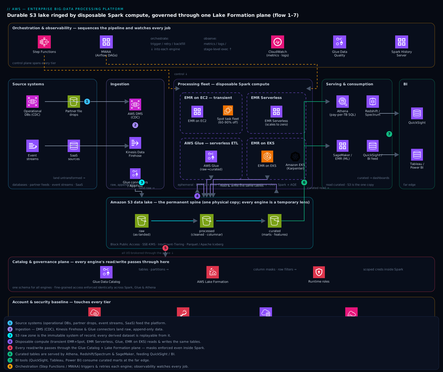
Tier 1 — Ingestion into the raw lake (S3). Source data lands, untransformed, in a raw zone on S3. Bulk and relational sources arrive via AWS DMS (CDC from operational databases) or direct S3 uploads/partner drops; high-volume event data arrives through Kinesis Data Firehose writing partitioned objects; SaaS sources come through AWS Glue connectors or AppFlow. Nothing is processed here. Raw is immutable, append-only, partitioned by ingest date, and is the system of record for replay — every derived dataset can be rebuilt from it.
Tier 2 — The lake on S3 (the spine). S3 holds the data across curated zones — raw (as-landed), processed/cleaned (conformed, deduplicated, columnar), and curated/aggregated (business-level marts and feature tables). Curated data is written as Parquet (columnar, compressed with zstd/Snappy) and, where transactional semantics matter, as Apache Iceberg tables. This is the one physical copy of all data; every compute engine is a temporary lens over it. (The storage design — zone layout, table formats, small-file economics — is the subject of the lakehouse reference; here we focus on the engines that read and write it.)
Tier 3 — The processing fleet: where the heavy lifting actually happens. This is the centre of gravity of this architecture and where it differs from every other data reference. Three Spark-capable compute shapes read the same S3 + catalog and write back the same tables, each chosen per workload:
- Amazon EMR on EC2 — transient clusters with instance fleets and Spot. The workhorse for large, scheduled, or long-running batch: the nightly multi-terabyte ETL, the monthly multi-month reprocessing, big Spark/ML feature pipelines. A cluster is launched for the job, runs Spark on a mix of On-Demand core nodes and Spot task nodes (60–90% cheaper), auto-scales to the data, and terminates on completion. You pay for minutes of actual compute, not a standing cluster.
- Amazon EMR Serverless — Spark with no cluster to manage. For spiky, intermittent, or unpredictable jobs where you don’t want to think about instance types at all. It provisions workers on demand, scales to zero between runs, and you pay per vCPU-second and GB-second of the job. Ideal for the ad-tech startup and for enterprise teams who want Spark without capacity planning.
- AWS Glue (serverless Spark ETL) — the managed pipeline engine. For the routine, declarative
raw → cleaned → curatedtransforms on a schedule or event. Glue is Spark under the hood but adds job bookmarks (incremental processing), built-in connectors, and tight orchestration. It’s the default for the steady-state pipeline; EMR is what you reach for when you need Spot economics, specific runtimes, or very large reprocessing.
A fourth shape, EMR on EKS, runs Spark as pods on a shared Amazon EKS cluster — the right answer when an org has standardised on Kubernetes and wants Spark to share capacity, tooling, and Karpenter-driven autoscaling with its other containerised workloads. All four write the same Parquet/Iceberg tables to the same Glue catalog; the engine is a per-workload choice, not a platform-wide religion.
Tier 4 — Catalog and governance (the plane underneath everything). The AWS Glue Data Catalog is the single technical metadata store — every table, schema, and partition registered once, read by EMR, Glue, Athena, and Redshift alike. AWS Lake Formation sits on top as the permission layer: it owns the S3 locations and grants database/table/column/row-level access rather than raw S3 access. Every engine — including an EMR cluster running Spark — vends credentials through Lake Formation at runtime, so “analysts cannot see the msisdn column; the EU team sees only EU rows” is enforced identically across Spark, Glue, and Athena.
Tier 5 — Serving and consumption (the right edge). Processed and curated tables are served to three patterns: Amazon Athena (serverless, pay-per-TB-scanned SQL for ad-hoc exploration and data-science queries — zero standing cost), Amazon Redshift / Spectrum (warehouse-grade BI over curated marts joined to hot dimensions), and Amazon SageMaker / EMR (reading curated feature tables directly for ML training). BI tools — QuickSight, Tableau, Power BI — sit beyond the engines. The data is never permanently copied into any engine; S3 is the one copy.
The two cross-cutting planes. Orchestration sits on top: AWS Step Functions and Amazon Managed Workflows for Apache Airflow (MWAA) sequence the pipeline — land raw, run Glue/EMR transforms, validate data quality, publish curated, then signal downstream — with retries, dependencies, and backfills. Observability spans everything: EMR/Glue push Spark metrics and logs to CloudWatch, the Spark History Server and EMR’s managed UIs expose stage-level execution, and Glue Data Quality gates the pipeline before bad data reaches consumers.
The diagram, in words. Picture a wide canvas. On the left, a column of source systems (databases, partner feeds, event streams, SaaS) with arrows through DMS / Firehose / Glue connectors into a single large S3 “raw” bucket. In the centre, S3 is drawn as the spine — three stacked buckets labelled raw → processed → curated, the unmistakable middle of the picture. Sitting above and around the S3 spine, four compute boxes all draw bidirectional arrows to S3: EMR on EC2 (drawn with a small On-Demand core block and a larger dashed “Spot task nodes” block to signal transience), EMR Serverless (a cloud with no fixed shape), AWS Glue (a gear), and EMR on EKS (Spark pods inside an EKS hexagon). Crucially, each compute box is drawn with a dashed border to convey ephemeral — they appear for a job and vanish. Underneath the entire spine runs a full-width band: Glue Data Catalog (one source of schema) with Lake Formation layered on it (the lock), and every compute box’s arrow to S3 passes through this band. On the right, Athena / Redshift / SageMaker read curated S3, feeding QuickSight / BI at the far edge. Across the top, an orchestration ribbon — Step Functions / MWAA (Airflow) — with control arrows reaching down into each compute box, and a parallel CloudWatch / Spark History / Glue Data Quality observability ribbon. Cross-cutting boxes at the very bottom — IAM Identity Center, KMS, VPC, CloudTrail — touch every tier. The defining visual: a permanent storage spine, ringed by disposable compute that is born and dies per job, all governed through one plane.
The ingestion menu in depth
Tier 1 named the three most common on-ramps — DMS, Firehose, and Glue connectors — but a real platform meets data wherever it lives, and “how does it get into the raw zone” is a decision you make per source, not once. Here is the fuller menu and when each is the right door.
| Source shape | Service | Why it fits |
|---|---|---|
| Operational database, ongoing change capture | AWS DMS (CDC) | Streams inserts/updates/deletes from Oracle/PostgreSQL/MySQL/SQL Server into S3 as they commit; full-load + ongoing replication |
| High-volume event/log streams | Amazon Data Firehose (formerly Kinesis Data Firehose) | Buffers and writes partitioned objects to S3 with no code; can convert JSON→Parquet in flight and now land directly into Iceberg tables |
| SaaS apps (Salesforce, ServiceNow, Zendesk) | Amazon AppFlow / Glue connectors | Managed, schema-aware pulls with no API client to write |
| On-prem file servers / HDFS / other object stores, online | AWS DataSync | Managed, accelerated, scheduled network copy over the internet or Direct Connect; handles NFS/SMB/HDFS/S3-compatible |
| Inbound files from external partners over SFTP/AS2 | AWS Transfer Family | Managed SFTP/FTPS/FTP/AS2 endpoints that land straight into S3 — no SFTP servers to run |
| Petabytes where the network would take weeks | AWS Snow Family (Snowball Edge) | Ship a physical, encrypted appliance; the wire is too slow or too costly for the first bulk load |
The decision that catches teams out is online vs. offline for the first big load. DataSync moves data over the network; Snowball ships a box. The rule of thumb is to estimate the transfer time first: 100 TB over a fully saturated 1 Gbps link is roughly 9 days of continuous transfer at ideal throughput, and real links rarely sustain ideal. If the initial copy would take more than a week or two — or if pushing it over the wire would blow your Direct Connect / internet-egress budget — ship a Snowball Edge for the historical backfill and use DataSync (or DMS CDC) for the ongoing delta. Meridian’s 12 PB history in the reference example is squarely Snow-family territory for the seed; the ~20 TB/day that lands afterward is DMS + Firehose.
Worked example — wiring one source correctly. The billing system is Oracle and must be captured continuously without a nightly full export hammering the OLTP database. The right pattern: an AWS DMS task in full-load + CDC mode reads the Oracle redo logs, does one initial full copy into raw/billing/, then streams every subsequent change as it commits. DMS writes CDC output to S3 as timestamped files partitioned by ingest date. A downstream Glue job then merges those change files into an Iceberg table in the processed zone with MERGE INTO, so updates and deletes are applied, not merely appended — turning an append-only change stream into a correct current-state table. The key insight: ingestion lands change events; the processing tier turns them into tables. Trying to make the ingestion layer emit perfectly-merged current state is where brittle pipelines come from.
Everything lands in the raw zone untransformed — and that immutability is exactly what lets you replay. If a merge-logic bug corrupts the processed billing table six months from now, the fix is to re-run the merge from raw, not to restore from backup, because raw is the system of record and every derived table is recomputable from it.
Component breakdown
| Component | Role in the platform | Key configuration choices |
|---|---|---|
| Amazon S3 (zoned) | The permanent spine — one physical copy of raw/processed/curated data; every engine’s read/write target | Separate buckets/prefixes per zone; partition by date; S3 Intelligent-Tiering on raw; lifecycle to Glacier for cold; Block Public Access + SSE-KMS; columnar Parquet for processed/curated |
| EMR on EC2 (transient) | Heavy/scheduled Spark batch — big ETL, reprocessing, ML feature jobs; launched per job, terminated after | Instance fleets with diversified Spot for task nodes; On-Demand for primary/core; managed scaling; --auto-terminate; EMRFS + Glue Catalog; runtime roles for Lake Formation |
| EMR Serverless | Spark with no cluster to manage — spiky, intermittent, small-to-medium jobs; scales to zero | Pre-initialised capacity for latency-sensitive jobs vs. cold-start for cheap; per-job application; vCPU/GB-second billing; auto-stop idle apps |
| AWS Glue ETL | Serverless Spark for routine raw→processed→curated transforms and orchestration glue |
Glue 5.0 (Spark 3.5); job bookmarks for incremental; Auto Scaling workers; Flex execution for non-urgent jobs (cheaper); Glue connectors for sources |
| EMR on EKS | Spark-as-pods on a shared EKS cluster — for K8s-standardised orgs | Virtual clusters per team; Karpenter + Spot node pools; pod templates; shares tooling/observability with other containerised workloads |
| Apache Spark | The processing engine inside EMR/Glue/EKS — the distributed compute itself | Tune partitions/shuffle; Adaptive Query Execution (AQE) for skew + dynamic coalescing; broadcast joins for small dims; cache hot intermediates; EMR’s optimised Spark runtime |
| Glue Data Catalog | One technical metadata store every engine shares | One catalog per environment; databases per domain; crawlers for schema discovery on raw; tables registered natively for curated |
| Lake Formation | Governance plane — fine-grained, engine-agnostic permissions enforced even inside Spark | Register S3 locations; remove IAMAllowedPrincipals; LF-Tags for scale; column masking + row filters; EMR runtime role enforcement |
| Amazon Athena | Serverless ad-hoc SQL over processed/curated — the default exploration engine | Engine v3 (Trino); workgroups with per-query scan caps; results to dedicated S3; query-result reuse cache |
| Step Functions / MWAA | Orchestration — sequence, retry, branch, backfill the pipeline | Step Functions for AWS-native, event-driven flows; MWAA (Airflow) for complex DAGs/cross-system dependencies; both trigger EMR/Glue and gate on data quality |
| Glue Data Quality | Data-quality gates between zones, before bad data reaches consumers | DQDL rules on processed→curated; fail-fast on freshness/null-rate/referential checks; quality results to CloudWatch/EventBridge |
Why each is here, and the choices that matter:
S3 is the spine, and it never moves. Every other component in the diagram is disposable; S3 is the one thing that persists. Because raw is immutable and replayable, and processed/curated are recomputable from raw, S3 is simultaneously your storage, your backup substrate, and your DR foundation. The single most consequential storage choice for processing performance is columnar Parquet with compression and sensible partitioning: a Spark job that reads partition-pruned, predicate-pushed Parquet touches a fraction of the bytes of one reading raw JSON, which is the difference between a 20-minute job and a 3-hour one.
The three-plus-one compute shapes are the heart of the architecture — and choosing between them is the skill. This table is the decision most teams get wrong:
| If the workload is… | Run it on… | Because… |
|---|---|---|
| Large, scheduled, predictable (nightly multi-TB ETL); long reprocessing | EMR on EC2, transient + Spot | Best $/compute via Spot task nodes and instance-fleet diversification; cluster lives only for the job |
| Spiky, intermittent, unpredictable, or you don’t want to size instances | EMR Serverless | Scales to zero between runs; no capacity planning; pay per vCPU/GB-second of actual work |
| Routine declarative ETL on a schedule/event; incremental loads | AWS Glue | Job bookmarks, connectors, fastest to author; serverless; Flex for cheap non-urgent runs |
| Ad-hoc SQL exploration; “what’s in this table?” | Athena | Zero standing cost; pay per TB scanned; no Spark to manage at all |
| Your org runs everything on Kubernetes already | EMR on EKS | Spark shares capacity, Karpenter autoscaling, and tooling with other K8s workloads |
The anti-pattern is choosing one shape for everything: running ad-hoc exploration on a giant standing EMR cluster (you’ll pay for idle), or forcing a steady nightly ETL onto EMR Serverless when a transient Spot cluster would be 70% cheaper, or hand-managing EMR for a job Glue would author in an afternoon.
Transient EMR + instance fleets + Spot is where the money is saved. A transient cluster launches, runs, and self-terminates, so there is no idle cost. Instance fleets let you specify a target capacity and a menu of acceptable instance types across multiple AZs; EMR fills it from whatever Spot capacity is cheapest and available, dramatically reducing the chance that a Spot shortage stalls your job. The rule that keeps this reliable: primary and core nodes on On-Demand (they hold HDFS/shuffle data and the application master — losing them kills the job); task nodes on Spot (they only run compute — losing one just reruns its tasks). Get that split right and you capture 60–90% Spot savings on the bulk of the cluster without risking job completion.
Spark is the engine, and AQE is the feature that earns its keep. The classic big-data failure — one stage runs for hours while 199 of 200 tasks finished in seconds — is data skew: a single hot key (one giant advertiser, one heavy subscriber) lands all its rows on one executor. Spark’s Adaptive Query Execution detects skewed partitions at runtime and splits them, dynamically coalesces tiny shuffle partitions, and switches join strategies based on actual sizes — turning a class of six-hour-then-OOM jobs into ones that just finish. Combined with broadcast joins for small dimensions and right-sized shuffle partitions, AQE is the single highest-leverage Spark setting on this platform.
Glue Catalog is the contract; Lake Formation is the lock — and the subtlety is that it works inside Spark. On a self-managed Hadoop cluster, once a job has the cluster’s IAM role it can read any S3 it can reach — governance is coarse and per-cluster. Here, an EMR cluster runs with a runtime role, and Lake Formation vends scoped, temporary credentials per query even to Spark, so the same column mask that hides msisdn in Athena also hides it from a Spark SELECT on EMR. Policy lives in one place and is enforced everywhere, including the heavy-compute tier.
Orchestration is not optional at enterprise scale. A real pipeline is a DAG: land raw, dedupe, conform, join reference data, aggregate, validate, publish, notify. Step Functions expresses this as an AWS-native state machine (great for event-driven, EMR/Glue-centric flows); MWAA (managed Airflow) is the choice when you have complex cross-system dependencies, hundreds of DAGs, or a team already fluent in Airflow. Both give you retries, backfills, and the ability to rerun one failed step rather than the whole pipeline — and both gate on Glue Data Quality so a failed freshness or null-rate check stops the pipeline before bad data reaches a dashboard.
Open table formats and the medallion lake, in depth
The overview called the zones raw → processed → curated. That naming is one dialect of a pattern the industry more often calls medallion: bronze (raw, as-landed), silver (cleaned, conformed, deduplicated), and gold (curated business-level marts and features). Same idea — and it matters for a reason beyond tidiness: each promotion between zones is a quality and trust boundary. Bronze is faithful to the source, warts and all; silver is where schema is enforced and duplicates die; gold is what a dashboard or a model is allowed to touch. When someone asks “can I trust this number,” the honest answer is “it depends which zone it came from,” and the zone tells you.
Why plain Parquet files are not enough, and what an open table format adds. A directory of Parquet files has no notion of a transaction. Two jobs writing the same partition at once can leave a reader seeing half of each. There is no atomic “replace yesterday’s data,” no way to UPDATE or DELETE a single row for a GDPR erasure request without rewriting whole partitions by hand, and no reliable snapshot to query “as of last Tuesday.” An open table format — Iceberg, Hudi, or Delta Lake — adds a metadata layer on top of the Parquet files that gives you ACID transactions, row-level MERGE/UPDATE/DELETE, schema evolution, hidden partitioning, and time travel, while the data itself stays as open Parquet on S3 that any engine can read.
| Format | Origin & sweet spot | Notable strengths |
|---|---|---|
| Apache Iceberg | Netflix; the AWS-default open format | Hidden partitioning + partition evolution (change partitioning without rewriting queries), snapshot isolation, broadest AWS support (Athena, EMR, Glue, Redshift Spectrum, S3 Tables) |
| Apache Hudi | Uber; upsert- and streaming-heavy ingestion | Record-level indexing, copy-on-write vs. merge-on-read tradeoff, incremental pulls; strong when you ingest a firehose of updates |
| Delta Lake | Databricks; ubiquitous where Databricks runs | Transaction log (_delta_log), mature tooling, OPTIMIZE/Z-ORDER; first-class on Databricks, readable on EMR |
For a green-field AWS lake, Iceberg is the safe default — it has the deepest native integration across Athena, EMR, Glue, and Redshift Spectrum, and it is the format AWS chose for S3 Tables and SageMaker Lakehouse. Choose Hudi when your dominant pattern is high-frequency upserts / streaming CDC and you want record-level indexing; choose Delta when you are already a Databricks shop. The Deploy Apache Iceberg on S3 with Glue Catalog and compaction lesson works the Iceberg mechanics end to end.
S3 Tables — managed Iceberg storage. Announced at re:Invent 2024, Amazon S3 Tables is a purpose-built S3 bucket type (a “table bucket”) that stores Iceberg tables and runs the housekeeping for you: automatic compaction of small files, snapshot expiration, and unreferenced-file cleanup, with tighter integration into the Glue Data Catalog and Lake Formation. The pitch is that the two chores that wreck self-managed Iceberg lakes — small-file compaction and snapshot/garbage cleanup — become a managed background service, at the cost of some control and a storage-management fee. On a general-purpose bucket you own those maintenance jobs yourself.
The small-files problem, with the numbers. This is the single most common self-inflicted wound on a lake, so it is worth making concrete. Suppose a streaming job writes one 4 MB Parquet file every 10 seconds into a partition. After a day that partition holds ~8,600 files totalling ~34 GB. A Spark job that reads it must list every object (S3 LIST is paginated and not free), open every file (each open is a round-trip, and every Parquet file carries footer-parsing overhead), and it gets almost none of Parquet’s columnar benefit because each file is tiny. The same 34 GB written as ~34 files of ~1 GB reads dramatically faster — fewer LISTs, far fewer opens, bigger contiguous columnar reads, better predicate push-down. The fix is compaction: a scheduled job (or S3 Tables’ automatic compaction, or Iceberg’s rewrite_data_files) that rewrites many small files into few right-sized ones. The target from the implementation section — 128 MB–1 GB per file — is not a nicety; it is the difference between a query that scans efficiently and one that dies of a thousand paper cuts. Throwing a bigger cluster at a small-files problem does nothing, because the bottleneck is object count and metadata, not CPU.
Implementation guidance
Bucket and zone layout. Consistent prefixing across zones, partitioned for pruning:
s3://acme-bd-raw-<acct>/<source>/<table>/ingest_date=YYYY-MM-DD/
s3://acme-bd-processed-<acct>/<domain>/<table>/dt=YYYY-MM-DD/   # Parquet
s3://acme-bd-curated-<acct>/<domain>/<table>/                  # Parquet/Iceberg
Raw partitions by ingest date for cheap lifecycle and replay; processed/curated partition by the business date queries actually filter on. The processing rule of thumb: aim for 128 MB–1 GB Parquet files — too small and Spark wastes time on task overhead and S3 listing; too large and you lose parallelism.
Terraform is the right IaC here (the team standardises on it). Manage as code:
- S3 buckets + Block Public Access + SSE-KMS + lifecycle/Intelligent-Tiering (
aws_s3_bucket,aws_s3_bucket_lifecycle_configuration). - Glue databases, catalog, and crawlers (
aws_glue_catalog_database,aws_glue_crawler); Glue jobs and triggers (aws_glue_job,aws_glue_trigger) with bookmarks enabled. - EMR: for persistent infra,
aws_emr_clusteror — better for transient jobs — define the cluster spec in the Step Functions / MWAA task so it’s created and torn down per run rather than living in Terraform state. For EMR Serverless,aws_emrserverless_application. For EMR on EKS,aws_emrcontainers_virtual_clusterover an existing EKS cluster. - Lake Formation:
aws_lakeformation_resourceto register each S3 location,aws_lakeformation_lf_tagfor the taxonomy,aws_lakeformation_permissions/aws_lakeformation_lf_tag_policyfor grants. Critically, remove theIAMAllowedPrincipalsdefault or IAM still grants broad access and your fine-grained policy is decorative. - Orchestration:
aws_sfn_state_machinefor Step Functions oraws_mwaa_environmentfor managed Airflow; Athena workgroups (aws_athena_workgroup) with per-query scan caps.
Transient EMR cluster spec — the choices that matter (expressed conceptually; this lives in the orchestration step, not standing infra):
{
  "ReleaseLabel": "emr-7.5.0",                 // Spark 3.5, optimised runtime
  "Applications": ["Spark"],
  "AutoTerminationPolicy": { "IdleTimeout": 600 },  // die if idle 10 min
  "ManagedScalingPolicy": { "MinCapacity": 2, "MaxCapacity": 64 },
  "Instances": {
    "InstanceFleets": [
      { "InstanceFleetType": "MASTER", "TargetOnDemandCapacity": 1,
        "InstanceTypeConfigs": [ { "InstanceType": "m6g.xlarge" } ] },
      { "InstanceFleetType": "CORE",   "TargetOnDemandCapacity": 2,   // On-Demand: holds data
        "InstanceTypeConfigs": [ { "InstanceType": "r6g.2xlarge" } ] },
      { "InstanceFleetType": "TASK",   "TargetSpotCapacity": 40,      // Spot: pure compute
        "InstanceTypeConfigs": [                                       // diversified menu
          { "InstanceType": "r6g.4xlarge" }, { "InstanceType": "r5.4xlarge" },
          { "InstanceType": "r6i.4xlarge" }, { "InstanceType": "m6g.8xlarge" }
        ],
        "LaunchSpecifications": { "SpotSpecification": {
          "AllocationStrategy": "price-capacity-optimized" } } }   // best Spot strategy
    ]
  },
  "Configurations": [ { "Classification": "spark-defaults", "Properties": {
    "spark.sql.adaptive.enabled": "true",
    "spark.sql.adaptive.skewJoin.enabled": "true",            // the skew killer
    "spark.sql.adaptive.coalescePartitions.enabled": "true",
    "spark.dynamicAllocation.enabled": "true"
  } } ]
}
The headline decisions: price-capacity-optimized Spot allocation (balances cheapest with least-likely-to-be-interrupted), On-Demand core / Spot task split, managed scaling so the cluster grows to the data and shrinks after, auto-termination so it never idles, and AQE on so skew and small-partition problems resolve at runtime.
EMR Serverless removes all of the above for spiky jobs — you submit a Spark job to an application and AWS handles workers:
aws emr-serverless start-job-run \
  --application-id <app> --execution-role-arn <runtime-role> \
  --job-driver '{ "sparkSubmit": {
      "entryPoint": "s3://acme-bd-code/jobs/daily_rollup.py",
      "sparkSubmitParameters": "--conf spark.sql.adaptive.enabled=true" } }'
Use pre-initialised capacity when a job is latency-sensitive (workers stay warm); accept cold-start when it’s a cheap background job.
Networking. Keep all data-plane traffic on the AWS backbone via a VPC Gateway Endpoint for S3 (free) and Interface (PrivateLink) endpoints for Glue, Lake Formation, Athena, KMS, STS, and the EMR APIs. EMR clusters, EMR Serverless, and EMR-on-EKS nodes run in private subnets with no public IPs; a NAT gateway handles only OS/package egress. The result: terabytes of shuffle and S3 I/O never traverse the public internet, and you avoid per-GB internet data charges on the heaviest traffic in the system.
Identity wiring. Human access flows from the IdP (the org standardises on Entra ID) through IAM Identity Center (SAML/SCIM) → permission sets → data-access roles, which are then granted Lake Formation permissions (not S3 permissions). Pipeline identities are scoped per engine: each Glue job, each EMR cluster (via its runtime role), and each EMR Serverless application gets its own role with only the Lake Formation grants it needs. No human or job role gets direct s3:GetObject on the lake buckets — Lake Formation vends scoped, temporary credentials per query, even into Spark. This is the wiring decision that makes governance real rather than theatrical, and it’s the one that most distinguishes this from a legacy Hadoop cluster where the cluster role could read everything.
A worked example: reading a Spark job, and what it costs
Two things separate people who use this platform from people who merely provision it: the ability to read why a Spark job is slow, and the ability to put a dollar figure on the compute choice. Here is one of each, worked end to end.
Reading a skewed join, step by step
The scenario: nightly, you join a 2 TB impressions table to a 500 MB advertisers dimension, group by advertiser, and write daily rollups. It ran in 40 minutes for months, then one week it takes 5 hours and sometimes OOM-kills at 95%. Nothing about the cluster changed. Walk it through:
- The join.
advertisersis 500 MB — larger than Spark’s default broadcast threshold (spark.sql.autoBroadcastJoinThreshold, default 10 MB), so Spark plans a shuffle (sort-merge) join: both sides are hash-partitioned byadvertiser_idacross (by default) 200 shuffle partitions, and matching keys are shipped to the same partition. So far, normal. - The skew. One advertiser — a giant retail brand — accounts for 22% of all impressions. Every one of those rows hashes to the same shuffle partition. So 199 partitions get ~9 GB each and finish in a minute, while one partition gets ~450 GB and lands on a single executor. That one task runs for hours; the stage cannot finish until it does; and if the executor’s memory + local disk cannot hold ~450 GB of shuffle, it spills and eventually OOMs. This is data skew, and “199 of 200 tasks done in seconds, one running for hours” is the signature you learn to recognise in the Spark UI.
- The fix — AQE skew join. With
spark.sql.adaptive.enabled=trueandspark.sql.adaptive.skewJoin.enabled=true, Spark measures partition sizes at runtime and, when a partition exceeds bothskewedPartitionThresholdInBytes(default 256 MB) andskewedPartitionFactor× the median partition size (default factor 5), it splits that partition into several and replicates the matching dimension rows to each — so the hot advertiser is processed by many tasks in parallel instead of one. The 5-hour job returns to ~40 minutes without you touching a line of business logic. - The other lever — broadcast. The 500 MB dimension only needed a shuffle because it was “big.” If you project it to just the columns and rows actually used (say 40 MB) and raise the broadcast threshold, Spark can broadcast the dimension to every executor and skip the shuffle entirely — no skew is possible, because the big side is never shuffled. Broadcasting is the cheapest join when one side is small; the art is knowing when a side is small enough.
The lesson: skew is a data-distribution problem, not a capacity problem. A bigger cluster gives the hot partition a bigger single executor, buying a little headroom before OOM, but it never parallelises that one task — only splitting the partition (AQE), changing the join (broadcast), or pre-salting the key does. That is why “the job is slow, add nodes” is the most expensive way to not fix a skewed job.
Costing the compute choice
Now the money. The same nightly job, four ways, on a representative ~40-node r6g.4xlarge-class footprint that runs ~1 hour a night. Figures are illustrative — regions and rates vary, so check current pricing — but the ratios are the point, and they hold everywhere. Assume ~$1 per node-hour On-Demand (EC2 + the EMR uplift) and Spot at ~30% of that.
| Option | What you pay for | Rough monthly cost | Notes |
|---|---|---|---|
| Standing cluster 24/7 | 40 nodes × 24 h × 30 d | ~$29,000 | Idle 23 h/day; the legacy default |
| Transient EMR, On-Demand only | 40 nodes × 1 h × 30 d | ~$1,200 | No idle — the structural win |
| Transient EMR, Spot task nodes | ~4 On-Demand core + ~36 Spot task | ~$350–500 | 60–90% off the compute bulk; the production default |
| EMR Serverless | vCPU-second + GB-second of the job | ~$500–700 | No sizing at all; slightly dearer than tuned Spot for a steady large job |
Two conclusions fall out. First, the giant saving is transience, not tuning: moving from a standing cluster to any transient option removes ~95% of the bill by deleting idle — that is the ~$29,000 → ~$1,200 step, and it is why the whole architecture exists. Second, among the transient options the choice is economic, not moral — Spot on a right-sized transient cluster is cheapest for this steady, predictable, large job, which is exactly why Meridian ran its nightly job on transient EMR + Spot and reserved Serverless for the unpredictable analyst jobs where “scale to zero, no sizing” beats Spot’s slightly lower rate. Add the Athena serving path — $5 per TB scanned (representative), cut ~90%+ by Parquet + partition pruning + compression — and the platform’s entire cost story is three multiplications you can do on a napkin.
Enterprise considerations
Security and Zero Trust. The model is “no implicit S3 access; every read — including from Spark — is brokered.” Concretely: (1) Block Public Access on every bucket, account-wide; (2) SSE-KMS with separate CMKs per zone for independent revocation and per-zone CloudTrail audit; (3) Lake Formation as the only path to data, so even an EMR cluster’s runtime role holds Lake Formation grants, not bucket policies; (4) column masking on PII (msisdn, imsi, card_pan) and row filters for tenancy/region, enforced in Spark, Glue, and Athena alike; (5) all traffic on PrivateLink; (6) EMR security configurations add in-transit and at-rest encryption for the cluster’s own intermediate data (local disks, shuffle); (7) CloudTrail data events + Lake Formation’s audit log give a complete “who processed/read which column when” trail. LF-Tags keep this scalable — tag a table confidentiality=pii once and grant on the tag, so new tables inherit policy automatically.
Cost optimization — this is the platform’s reason to exist, and it’s layered.
- The structural win (transience): transient EMR and scale-to-zero EMR Serverless mean you pay for compute only while a job runs. The telco that ran a 400-node cluster at 30% utilisation 24/7 now pays for ~30% of that capacity, ~30% of the day — a step-change, not a tuning gain.
- Spot on the bulk of the cluster: diversified Spot task fleets save 60–90% on the compute majority of every transient cluster, with On-Demand core nodes protecting completion.
- Right-sized compute per job: the spiky job goes to Serverless (no idle), the routine ETL to Glue Flex (cheaper non-urgent execution), the ad-hoc query to Athena (no cluster at all). Each lands on its cheapest correct shape.
- Storage tiering and scan reduction: Intelligent-Tiering on raw, Glacier lifecycle on cold; Parquet + compression + partition pruning cut both Spark read time and the Athena pay-per-TB bill by 90%+ versus raw formats. Athena workgroup per-query scan caps stop a runaway
SELECT *from costing thousands. - Graviton everywhere: ARM-based Graviton instance types (
m6g/r6g) for EMR deliver materially better price-performance than x86 for Spark — often 20%+ — and Spark runs on them unchanged.
Scalability. S3 absorbs effectively unlimited objects and throughput; partition-prefix design avoids hotspots. EMR managed scaling grows a cluster mid-job as a stage demands more executors and shrinks it after; EMR Serverless and Glue absorb concurrency automatically; Athena is serverless. The real scaling discipline is not capacity — it’s data engineering: keeping Parquet file sizes in the sweet spot (compaction jobs to fix small files), partitioning on the columns queries filter, and handling skew with AQE so adding nodes actually helps instead of one hot key bottlenecking on one executor regardless of cluster size. Throwing hardware at a skewed job is the most expensive way to not fix it.
Reliability and DR (RTO/RPO).
- Job-level resilience: transient clusters tolerate Spot interruptions because task nodes are disposable (their tasks rerun) and core/AM nodes are On-Demand. Orchestration retries individual failed steps, not whole pipelines, and idempotent, partition-overwrite writes mean a rerun produces the same result rather than duplicates.
- Data durability and DR: S3 is 11 nines; Cross-Region Replication on the raw zone (the system of record) gives geographic protection. Because processed/curated are recomputable from raw, you replicate the irreplaceable layer and rebuild the rest by re-running pipelines in the DR region.
- The catalog is the subtle DR risk: it lives in Glue/Lake Formation, not S3, so export catalog definitions and Lake Formation grants via IaC so the metadata layer is reproducible in DR — a lake with no catalog is opaque files.
- Targets: with CRR + IaC-reproducible catalog + code-as-pipelines, a realistic posture is RPO ≈ 15 min for raw (replication lag) and RTO of a few hours in a region failure — re-point the catalog, relaunch transient clusters, re-run pipelines to rebuild curated from replicated raw. There is no standing cluster to fail over because there is no standing cluster.
Observability. EMR and Glue emit Spark metrics and driver/executor logs to CloudWatch; the Spark History Server (and EMR’s managed Spark UI / Persistent UIs) expose stage-level execution — the single most important diagnostic for “why is this job slow,” surfacing spills, skew, and shuffle volume. Glue Data Quality (DQDL) gates the processed→curated boundary so freshness/null-rate/referential failures stop the pipeline and fire EventBridge alerts before bad data reaches dashboards. Track four SLOs: pipeline freshness (curated lag), job cost (compute-hours and bytes scanned/day), data-quality pass rate, and Spot interruption rate (rising interruptions are a signal to broaden the instance-fleet menu).
Governance. Lake Formation LF-Tags are the scalable model — a taxonomy (domain, confidentiality, retention) applied to databases/tables, grants written against tags so policy is inherited not hand-maintained. This is also the foundation for a data-mesh evolution: each domain owns its processed/curated databases and the jobs that produce them, sharing across domains via Lake Formation cross-account grants, with a central platform team owning only the tag taxonomy, the orchestration substrate, and the EMR/Glue golden patterns. Pair with Amazon DataZone for business-level discovery and access requests on top of the technical Glue catalog.
Reference enterprise example
Meridian Telecom is a fictional mobile carrier with 62M subscribers, running the legacy mess described at the top: a 400-node on-prem Hadoop cluster built in 2017, ~600 TB/month landing (call-detail records, RAN telemetry, billing events, app analytics), 12 PB at rest, ~30% average utilisation because it’s sized for the monthly fraud-reprocessing peak. The data-platform run-rate (hardware amortisation, datacentre, ops staff, Hadoop support) is ~$6.4M/year, three teams are queued for capacity that doesn’t exist, and the last audit flagged that the cluster role could read subscriber imsi/msisdn with no fine-grained control.
What they built. Over three quarters they migrated to the architecture above:
- Ingestion: DMS CDC from the Oracle billing system and the Postgres CRM into
raw; Firehose for the ~9B/day network-event and app-analytics records; partner mediation files dropped directly to S3. Raw landed ~20 TB/day, partitioned by ingest date, on Intelligent-Tiering with Glacier lifecycle past 18 months. - Lake: ~12 PB migrated to S3 over the period; processed/curated written as Parquet (zstd), ~1.4 PB, partitioned by date and region.
- Processing — the heart of it:
- The nightly CDR conformance + dedupe + enrichment pipeline (the old 7-hour job) ran on a transient EMR-on-EC2 cluster:
m6gprimary,r6g.2xlargeOn-Demand core, and a diversified Spot task fleet (~50r6g/r6i/r5nodes,price-capacity-optimized) that managed-scaled to the night’s volume and self-terminated by 04:30. Spark AQE eliminated the skew from a handful of high-volume corporate accounts that used to OOM the job. - The monthly 14-month fraud-detection reprocessing ran on a larger transient cluster for ~5 hours once a month — capacity that previously dictated the entire cluster’s 24/7 size, now summoned and released on demand.
- The routine reference-data and aggregate jobs moved to Glue 5.0 with job bookmarks; ad-hoc and unpredictable analyst jobs went to EMR Serverless (scale-to-zero).
- Orchestration: MWAA (Airflow) ran the ~120-DAG pipeline with per-step retries, backfills, and Glue Data Quality gates on the
processed→curatedboundary.
- The nightly CDR conformance + dedupe + enrichment pipeline (the old 7-hour job) ran on a transient EMR-on-EC2 cluster:
- Governance: Lake Formation with LF-Tags (
domain,confidentiality,retention);subscriber.imsi,subscriber.msisdn, andbilling.card_pancolumn-masked for analysts; a row filter restricted the EU MVNO team to EU subscribers. All legacy direct-S3 access was removed and re-granted through Lake Formation runtime roles — including for the EMR clusters. - Consumption: Athena for the ~180-person analytics/DS org (no more cluster contention); Redshift Serverless for the ~60 executive QuickSight dashboards over curated marts; SageMaker on curated feature tables for the churn and fraud models.
Decisions worth noting. They put core nodes on On-Demand and task nodes on Spot after an early pilot where an all-Spot cluster lost its core nodes mid-job and had to restart from scratch. They standardised on Graviton (m6g/r6g) for ~22% better Spark price-performance. They chose transient EMR over EMR Serverless for the predictable nightly job because Spot on a right-sized fleet was ~65% cheaper than Serverless for that steady, large workload — but used Serverless for the unpredictable analyst jobs where no-idle beat Spot pricing. They turned AQE skew-join on after the corporate-account skew turned a 40-minute job into a 5-hour one in week two. They set Athena workgroup scan caps at 3 TB after an analyst’s SELECT * scanned 50 TB.
The outcome (12 months).
- Platform run-rate fell from ~$6.4M to ~$2.7M/year (~58%) — overwhelmingly from killing 24/7 peak-sized capacity (transient + scale-to-zero), Spot on the compute bulk, and Graviton.
- The nightly pipeline finished by 04:30 instead of mid-morning, and stopped failing twice a week — orchestration retries plus AQE skew handling made it boring.
- Scaling became an API call: the three queued teams got capacity the same week by launching their own transient clusters against the same lake, rather than waiting on an 18-month hardware refresh.
- The PII audit finding closed: one Lake Formation report now answers “who can read
imsi” across Spark, Glue, and Athena — and the masks are enforced inside the Spark jobs, not just in the BI layer. - DR: raw CRR to a second region + IaC-reproducible catalog + code-as-pipelines gave a tested RPO ≈ 15 min / RTO ≈ 3 h, with no standing cluster to fail over.
Going deeper
The overview is enough to build the platform. This section is for the engineer who has to operate it — the internals, the newer AWS direction, and the edges where things break.
How Lake Formation enforces security inside Spark
The claim that “the same column mask hides msisdn in Athena and in a Spark SELECT on EMR” sounds like magic; the mechanism is credential vending. Normally an engine reads S3 with its own IAM role. Under Lake Formation you register the S3 locations and remove the IAMAllowedPrincipals grant — the backward-compatibility default that lets plain IAM keep working. Leave it in place and your fine-grained policy is decorative, because IAM still grants broad access. Now, when an engine wants data, it does not read S3 directly; it calls Lake Formation (GetDataAccess, and for table access GetTemporaryGlueTableCredentials), Lake Formation checks the caller’s grants, applies column filters and row filters, and hands back short-lived, scoped credentials plus a filtered view of the data. For EMR this rides on the cluster’s runtime role (not its instance profile) and record-server machinery that applies the filtering before rows reach the Spark executors. The upshot: policy lives once in Lake Formation and is enforced at the storage boundary, so it cannot be bypassed by “just reading the bucket.” The wiring rule that makes it real: no human or job role gets direct s3:GetObject on the lake buckets — every read is brokered.
Spot interruption mechanics, and why the node split matters
EC2 Spot capacity is reclaimed when AWS needs it back; you get a two-minute interruption notice (and a rebalance recommendation earlier). On EMR, losing a task node is a non-event — its in-flight Spark tasks are simply rescheduled elsewhere, because task nodes hold no durable state. Losing a core node is different: core nodes carry HDFS blocks and shuffle data, so their loss can force recomputation or, if you lose enough, fail the job. That asymmetry is the entire reason for the core-on-On-Demand, task-on-Spot rule. The price-capacity-optimized allocation strategy (the current best default) picks Spot pools that are both cheap and deep, minimising interruptions versus the older lowest-price strategy, which piles into one cheap-but-shallow pool and gets mass-reclaimed. Diversify the task fleet across many instance types and AZs so no single pool’s reclamation can stall the job. The EC2 Spot with mixed instances and capacity-optimized allocation lesson covers the interruption-handling patterns in depth.
The warehouse edge: Redshift, in depth
“Redshift / Spectrum” in the serving tier hides several distinct choices. RA3 nodes decouple compute from storage: data lives in Redshift Managed Storage (RMS), an S3-backed tier, so you size compute and storage independently and stop over-provisioning nodes just to hold bytes. Redshift Spectrum queries S3 data directly as external tables (via the Glue catalog) without loading it — the warehouse reaches into the lake. Redshift Serverless removes cluster management entirely, billing by RPU-seconds and scaling on demand — the natural fit for spiky BI. And Zero-ETL integrations replicate data from Aurora (MySQL/PostgreSQL), RDS for MySQL, and DynamoDB into Redshift in near-real-time without you building a pipeline — the source keeps serving transactions while an analytics-ready copy stays fresh in the warehouse. Zero-ETL is AWS quietly deleting an entire category of glue code; where it fits, prefer it over hand-built CDC into Redshift.
The newer direction: SageMaker Lakehouse and Unified Studio
The strategic shift worth knowing: AWS is unifying the lake and the warehouse. Amazon SageMaker Lakehouse presents S3 data-lake tables and Redshift warehouse tables through one Iceberg-compatible access layer, governed by Lake Formation — so a single engine can query across lake and warehouse without copying data between them. Amazon SageMaker Unified Studio (announced at re:Invent 2024, generally available in 2025) then wraps data engineering, SQL analytics, ML, and generative AI into one studio over that lakehouse, with Amazon DataZone’s business catalog and governance folded in. You do not have to adopt it to run the architecture in this lesson — but it is the direction the individual services (Glue, Athena, EMR, Redshift, Lake Formation, DataZone) are converging toward, and green-field platforms should expect “lake vs. warehouse” to become one governed surface rather than two.
Search, NL, and the rest of the serving edge
Beyond SQL and BI, two serving patterns recur. Amazon OpenSearch Service is the target when the access pattern is full-text search or log/observability analytics — curated data (or a Firehose branch) flows into OpenSearch for sub-second search and dashboards, complementing rather than replacing Athena’s scan-based SQL; OpenSearch also has a zero-ETL integration to query S3 directly. Amazon Q brings natural language over the top: Q in QuickSight answers “why did revenue dip in APAC” the way an analyst would, and generative SQL in Athena/Redshift turns plain-English questions into queries. These are consumption conveniences layered on the same governed curated tables — they change who can ask, not where the data lives.
Orchestration: three tools, one job
Step Functions, MWAA, and Glue workflows overlap, and picking between them is about blast radius. Glue workflows chain Glue jobs, crawlers, and triggers into a DAG inside Glue — simplest when the whole pipeline is Glue. Step Functions is the AWS-native state machine for event-driven flows that span services (EMR, Glue, Lambda, ECS) with visual retries and error handling — see Step Functions distributed orchestration. MWAA (managed Airflow) wins when you have hundreds of DAGs, complex cross-system dependencies, backfills, and a team already fluent in Airflow’s Python-DAG idiom. Small pipeline: Glue workflows. AWS-native event flow: Step Functions. Big heterogeneous DAG estate: MWAA.
Batch vs. stream: the lambda/kappa framing and where Flink sits
This whole lesson is the batch half — Spark transforming bounded datasets on disposable compute. The complement is stream processing: unbounded event data handled record-by-record at low latency, whose AWS engine is Amazon Managed Service for Apache Flink (formerly Kinesis Data Analytics for Apache Flink). Two classic blueprints frame the choice. Lambda architecture runs both a batch layer (accurate, high-latency — this platform) and a speed layer (fast, approximate — Flink/streaming) and merges them at serving time; it is powerful, but you maintain two codebases. Kappa architecture says “treat everything as a stream,” running a single streaming pipeline and replaying history through the same code when you need a recompute — simpler, but not every heavy transform fits a streaming model. Most enterprises land in between: batch for the heavy, correctness-critical transforms here; streaming on the real-time architecture for sub-second reactions; one shared S3 lake and catalog underneath both.
Quotas, limits, and the edges that bite
A few real limits worth internalising before they surprise you in production. EMR and EMR Serverless consume EC2 vCPU service quotas — a large transient cluster can hit an account vCPU ceiling and simply fail to scale, so raise quotas before the month-end peak, not during it. Athena enforces per-query and per-workgroup limits plus DML concurrency caps; a fleet of analysts can queue behind them, which is a signal to split workgroups. Glue has a default concurrent-run limit per job and DPU quotas. Lake Formation caps the number of filters and tags. And the subtle DR edge from the reliability section bears repeating: the catalog and Lake Formation grants do not live in S3 — they live in Glue/Lake Formation and must be reproduced by IaC in a DR region, or you fail over to a lake of opaque files with no schema and no policy.
When to use it
Use this big-data processing platform when:
- You have large-volume batch transformation (terabytes-to-petabytes) that a single machine or a fixed cluster can no longer process in the time available.
- Your compute is provisioned for the peak and paid at the average — a standing cluster sized for the heaviest job, idle most of the time.
- You have heterogeneous workloads (scheduled ETL, spiky ad-hoc, periodic reprocessing, ML feature engineering) that one fixed cluster forces to contend.
- You want Spark’s power without operating Hadoop — managed EMR/Glue instead of a platform team babysitting YARN — and governance that reaches into the compute tier, not just the query layer.
Trade-offs and anti-patterns:
- Operational surface is data engineering, not server management. You trade YARN babysitting for file hygiene (Parquet sizing/compaction), partition design, skew handling, and an orchestration DAG. Anti-pattern: ignoring small files — millions of tiny Parquet objects from frequent writes will make every Spark job and Athena query slow regardless of cluster size; scheduled compaction is mandatory.
- All-Spot is a trap on the wrong nodes. Anti-pattern: putting core/primary nodes on Spot — losing them kills the job and you restart from zero. Core/AM on On-Demand, task on Spot.
- Throwing hardware at skew doesn’t work. Anti-pattern: scaling up a cluster to “fix” a slow job that’s actually skewed — one hot key bottlenecks on one executor no matter how big the cluster. Fix it with AQE/salting, not nodes.
- Don’t run interactive, sub-second workloads here. EMR/Glue/Athena are batch-to-interactive-SQL (seconds-to-hours). Sub-second operational lookups belong on DynamoDB/Aurora; sub-second event reaction belongs on the streaming architecture.
- Don’t choose one engine for everything. Forcing ad-hoc onto a standing cluster, or steady ETL onto Serverless, or hand-managing EMR for a Glue-shaped job, all leave money or simplicity on the table.
Alternatives and how to choose:
| Situation | Better fit |
|---|---|
| Sub-second event reaction is the core need (fraud-in-flight, live dashboards) | Kinesis + Flink / Lambda — the real-time streaming architecture |
| The need is storage design — open tables, store-once-query-many governance | Data Lakehouse on AWS (Iceberg + Lake Formation + multi-engine) |
| Pure SQL BI on modest, predictable volume; no Spark/ML | Redshift-only warehouse — fewer moving parts |
| Mostly ad-hoc SQL on S3, no heavy distributed transforms yet | Athena + Glue, defer EMR until jobs need Spark muscle |
| Want a managed lakehouse/Spark platform with less AWS plumbing, multi-cloud | Databricks on AWS (Unity Catalog + Delta + managed Spark) |
| Org runs everything on Kubernetes and wants Spark to share it | EMR on EKS as the processing tier of this same architecture |
The big-data processing platform on AWS is the right default when heavy, varied batch transformation over a growing dataset would otherwise force you to buy and run peak-sized compute around the clock. By keeping storage permanent on S3 and making compute disposable — transient EMR with Spot for the heavy lifting, EMR Serverless and Glue for the spiky and the routine, Athena for exploration, all governed through one Lake Formation plane — you process any volume on compute sized per job and billed by the second, and the cluster that used to cost the same in July as in December simply ceases to exist.
Practice challenges
Work these in order — they escalate from “read the model” to “make the production call.” Each has a solution with a one-line why.
1 (Beginner). In one sentence each, say which is permanent and which is disposable in this architecture, and name the AWS service for each.
<details><summary>Solution</summary>
Permanent = storage = Amazon S3 (the data-lake spine; it holds raw/processed/curated forever). Disposable = compute = EMR / EMR Serverless / Glue (Spark engines launched per job and terminated after). Why: the entire cost and scaling model follows from decoupling one permanent S3 copy from compute you pay for only while a job runs. </details>
2 (Beginner). You need to run an ad-hoc SELECT COUNT(*) ... WHERE dt='2026-09-01' once to answer a question. Which engine, and why not spin up EMR?
<details><summary>Solution</summary>
Use Amazon Athena — serverless, pay only for the TB scanned, nothing to provision or tear down. Why: a one-off query has zero justification for a Spark cluster; Athena has no standing cost, and partition pruning on dt means it scans one day, not the whole table.
</details>
3 (Intermediate). A nightly transient EMR cluster keeps failing when Spot capacity is tight, and when it does complete it sometimes restarts from scratch. The team put all nodes (primary, core, task) on Spot to save money. What is the fix, and what principle did they violate?
<details><summary>Solution</summary>
Put primary and core nodes on On-Demand and keep only task nodes on Spot, with a diversified instance-fleet menu and price-capacity-optimized allocation. Why: core/primary nodes hold HDFS/shuffle data and the application master — losing them to a Spot reclaim kills the job; task nodes are pure compute, so losing one just reruns its tasks.
</details>
4 (Intermediate). A Spark stage shows 199 of 200 tasks finishing in seconds and one task running for two hours before the job OOMs. Diagnose it, and give the setting that fixes it without adding nodes.
<details><summary>Solution</summary>
It is data skew — one hot key hashed all its rows into a single shuffle partition on one executor. Enable Adaptive Query Execution with skew-join handling: spark.sql.adaptive.enabled=true and spark.sql.adaptive.skewJoin.enabled=true, so Spark splits the oversized partition at runtime. Why: a bigger cluster only gives the one hot task a bigger executor; only splitting the partition (or broadcasting/salting) parallelises it.
</details>
5 (Advanced). Design the compute assignment for four workloads on one lake: (a) a predictable nightly 3 TB ETL, (b) unpredictable analyst Spark jobs a few times a week, © a routine incremental raw→processed load every hour, (d) “what’s in this table?” exploration. Assign an engine to each and justify.
<details><summary>Solution</summary>
(a) Transient EMR on EC2 + Spot — steady, large, predictable, so tuned Spot on a right-sized fleet is cheapest. (b) EMR Serverless — spiky and unpredictable, so scale-to-zero with no sizing beats paying for idle. © AWS Glue with job bookmarks — routine incremental ETL, fastest to author, serverless, Flex for cheap non-urgent runs. (d) Athena — zero standing cost, pay per TB scanned. Why: the engine is a per-workload economic choice; forcing one shape on all four leaves either money or simplicity on the table. </details>
6 (Advanced). After adopting Lake Formation, an auditor asks: “prove that analysts cannot read the msisdn column, including from Spark jobs on EMR, not just in the BI tool.” Explain the mechanism that makes this true and the one configuration mistake that would silently make it false.
<details><summary>Solution</summary>
Register the S3 locations with Lake Formation and grant column-level access; every engine — including EMR via its runtime role — obtains short-lived, scoped credentials from Lake Formation per query, and the column filter is applied at the storage boundary before rows reach the Spark executors, so the mask holds in Spark, Glue, and Athena identically. The silent failure: leaving the IAMAllowedPrincipals default grant in place (or granting any role direct s3:GetObject on the bucket), which lets plain IAM bypass Lake Formation and read the raw column. Why: fine-grained governance is only real if Lake Formation is the sole path to the data.
</details>
Common beginner mistakes
These are misconceptions, not error messages — the wrong mental model a beginner brings, and the right one to replace it with.
-
“Bigger cluster = faster job.” The instinct when a job is slow is to add nodes. But the two most common slowdowns — data skew and small files — do not respond to more hardware at all. A skewed job bottlenecks on one executor no matter how big the cluster; a small-files job is bound by object count and metadata, not CPU. Right model: diagnose why it is slow in the Spark UI first (skew? spill? small files?), then apply the matching fix (AQE, compaction, broadcast) — nodes are the last lever, not the first.
-
“The cluster should stay up so jobs start fast.” Keeping an EMR cluster running “so we don’t wait for it to launch” reintroduces the exact idle cost the architecture exists to kill. Right model: compute is disposable — launch transient clusters per job (or use EMR Serverless / Glue), and if cold-start latency genuinely matters, use EMR Serverless pre-initialised capacity, not a standing cluster running 24/7.
-
“Lake Formation is set up, so we’re governed.” Registering locations and writing column masks does nothing if the legacy
IAMAllowedPrincipalsgrant is still there, or a role still has directs3:GetObject— IAM quietly grants broad access and your masks become decorative. Right model: governance is real only when Lake Formation is the sole path to the data; remove direct bucket access from every human and job role. -
“We’ll just store the raw JSON and query it directly.” Querying raw JSON/CSV with Athena or Spark scans every byte of every file every time — slow, and on Athena’s pay-per-TB model, expensive. Right model: land raw as-is for replay, but convert to columnar Parquet with compression and partitioning in the processed zone; a partition-pruned, predicate-pushed Parquet read touches a fraction of the bytes.
-
“One engine (or one table format) for everything.” Beginners pick EMR or Glue or Athena as “the tool” and force every workload onto it. Right model: they are complementary — Athena for exploration, Glue for routine ETL, transient EMR+Spot for heavy predictable batch, EMR Serverless for spiky — all chosen per workload against one shared lake and catalog.
-
“Adding streaming would make this real-time.” Bolting a streaming engine onto a batch platform to “make it faster” misunderstands the split: this platform is for heavy, correctness-critical, bounded transforms measured in minutes-to-hours. Right model: sub-second reactions belong on the streaming architecture (Kinesis + Managed Service for Apache Flink); batch and stream share the S3 lake but answer different questions — don’t force one to do the other’s job.
Glossary
- Apache Spark — the distributed processing engine that splits a transformation across many machines; the compute inside EMR, EMR Serverless, and Glue.
- Amazon EMR — AWS’s managed Hadoop/Spark platform. EMR on EC2 runs Spark on rented servers (transient clusters + Spot); EMR Serverless runs Spark with no cluster to manage; EMR on EKS runs Spark as pods on Kubernetes.
- Transient cluster — an EMR cluster launched for a single job and terminated on completion, so it costs nothing when idle. The opposite of a standing/persistent cluster.
- AWS Glue — serverless managed Spark for routine
raw→processed→curatedETL; adds job bookmarks (incremental processing) and built-in connectors. - Amazon Athena — serverless SQL over S3; you pay per TB scanned, with no cluster to run. Athena engine v3 is Trino-based.
- Amazon S3 — object storage; here, the permanent data-lake spine that every compute engine reads and writes.
- Data lake — one durable copy of all data on S3, queried in place by many engines, rather than loaded into a single database.
- Medallion / zones (raw → processed → curated, a.k.a. bronze/silver/gold) — the promotion tiers of the lake: as-landed, cleaned/conformed, business-ready. Each boundary is a quality gate.
- Parquet — a columnar, compressed file format; reading it with partition pruning and predicate push-down touches a fraction of the bytes of raw JSON/CSV.
- Partitioning — organising files into prefixes (e.g.
dt=2026-09-01) so a query filtered on that column reads only the relevant folders — “partition pruning.” - Open table format (Iceberg / Hudi / Delta) — a metadata layer over Parquet files adding ACID transactions, row-level
MERGE/UPDATE/DELETE, schema evolution, and time travel. Iceberg is the AWS default. - Amazon S3 Tables — a purpose-built S3 bucket type for Iceberg tables that runs compaction, snapshot expiration, and cleanup as a managed service.
- Glue Data Catalog — the shared technical metadata store (databases, tables, schemas, partitions) every engine reads, so they all see the same tables.
- AWS Lake Formation — the governance plane: fine-grained (database/table/column/row) permissions enforced across every engine, including inside Spark, via credential vending.
- LF-Tags — Lake Formation tags (e.g.
confidentiality=pii) you grant against, so new tables inherit policy automatically instead of by hand-maintained grants. - Runtime role — the IAM role an EMR cluster/job assumes per job to obtain Lake Formation-scoped credentials, rather than using the cluster’s broad instance profile.
- Spot instances — spare EC2 capacity at 60–90% off, reclaimable with a 2-minute notice; used for EMR task nodes (disposable), never core/primary.
- Instance fleet — an EMR capacity spec listing a menu of acceptable instance types across AZs, filled from whichever Spot pools are cheapest and deepest (
price-capacity-optimized). - Data skew — when one hot key sends most rows to a single shuffle partition/executor, so one task runs for hours; fixed by AQE skew-join, broadcast, or salting — not by more nodes.
- Adaptive Query Execution (AQE) — Spark’s runtime optimiser that splits skewed partitions, coalesces tiny ones, and switches join strategies based on the data’s actual sizes.
- Shuffle vs. broadcast join — a shuffle join repartitions both sides by the join key across the cluster (can skew); a broadcast join ships a small table to every executor and skips the shuffle.
- Small-files problem — thousands of tiny Parquet files that slow every read via
LIST/open overhead; fixed by compaction into 128 MB–1 GB files. - AWS DMS — Database Migration Service; captures ongoing changes (CDC) from operational databases into the raw zone.
- Amazon Data Firehose — (formerly Kinesis Data Firehose) buffers streaming events and writes partitioned objects to S3, optionally converting to Parquet or landing in Iceberg.
- Zero-ETL — near-real-time replication from Aurora/RDS/DynamoDB into Redshift with no pipeline to build.
- Redshift RA3 / Managed Storage / Spectrum / Serverless — RA3 decouples compute from S3-backed managed storage; Spectrum queries S3 in place; Serverless removes cluster management.
- Orchestration (Step Functions / MWAA / Glue workflows) — sequencing the pipeline DAG with retries, dependencies, and backfills; MWAA is managed Apache Airflow.
- Lambda vs. Kappa architecture — Lambda runs parallel batch + speed layers merged at serving; Kappa runs a single streaming pipeline and replays history through it.