A BigQuery bill blows up for two reasons: queries read far more bytes than they need to, and you are paying for compute on the wrong model. Both are fixable without rewriting your warehouse. This guide works from the physical layer up — partitioning and clustering to cut bytes scanned — then up to the capacity layer — editions, reservations, and autoscaling to cap and isolate compute — and closes with hard guardrails so a single bad query can never page you about the invoice again.
In a nutshell
A BigQuery bill is really two numbers multiplied by your carelessness: how many bytes each query reads, and which compute model you pay on. Get either wrong and the invoice balloons; get both right and a warehouse that scans terabytes stays cheap and fast. This lesson is the playbook for both — the physical table layout that shrinks the scan, and the capacity controls that cap and isolate the compute.
Think of a BigQuery table as a vast warehouse of numbered filing cabinets. Partitioning labels each cabinet by date (or ID range) so a query for “last Tuesday” walks straight to one cabinet and ignores the rest — it never even opens the others. Clustering then sorts the folders inside each cabinet so you skip whole drawers too. A careless SELECT * is an intern told to photocopy every page in the building to answer one question; a pruned, projected query sends them to one drawer for one folder. On the money side, on-demand pricing is paying the copy shop per page, while Editions/reservations is hiring a fixed crew of workers (slots) for the month — cheaper once the work is steady, wasteful if it is spiky.
The trap that catches everyone: a partitioned table is not automatically a pruned table. If your filter is written in a way the planner cannot resolve before the query runs — wrapping the partition column in a volatile function, comparing it to a subquery — BigQuery quietly falls back to reading the whole warehouse and bills you for it. Most runaway BigQuery bills are exactly this: good schema, defeated pruning. The rest of this guide is how to lay tables out so pruning engages, write queries that keep it engaged, reuse hot results instead of rescanning, and bolt on guardrails so a single bad query can never surprise you.
Level: Advanced · Time: ~30 min · You’ll need: comfort with BigQuery datasets, tables, and GoogleSQL queries, plus a rough grasp of what a “slot” and “bytes scanned” mean on your bill.
Prerequisites: the BigQuery deep dive for datasets, tables, slots, and the pricing surface this lesson tunes, and the Billing & cost management deep dive for budgets, billing export, and committed-use discounts. If you also govern who can read what, the sibling BigQuery fine-grained access lesson pairs naturally with the cost controls here.
After this lesson you can:
- Choose on-demand vs Editions/reservations from measured spend, not a guessed TiB threshold.
- Partition and cluster a table so filters prune partitions and skip blocks, and prove the win with a dry run.
- Write GoogleSQL that keeps pruning engaged, and cut compute with approximate aggregates.
- Reach for materialized views, BI Engine, and result caching to serve hot reads without rescanning storage.
- Cut the storage line with the logical-vs-physical billing model and long-term storage.
- Cap the ceiling with
require_partition_filter,maximum_bytes_billed, custom quotas, and budgets so a mistake cannot ruin the month.
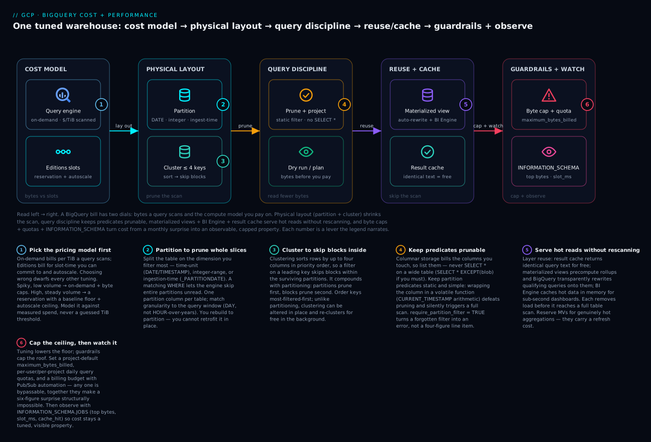
Read left → right: pick the pricing model, lay the table out so partitioning and clustering prune the scan, keep query predicates prunable, serve hot reads from materialized views, BI Engine, and the result cache instead of rescanning, then cap the ceiling with byte limits and quotas and watch it all through INFORMATION_SCHEMA — the six numbered levers map to the sections below.
1. Pick the right pricing model before you tune anything
BigQuery bills compute two ways, and choosing wrong dwarfs every other optimization.
- On-demand: you pay per TiB of data scanned by queries (storage is billed separately). Zero capacity to manage, but cost is a direct function of bytes read, and a single
SELECT *over a fat table can cost real money. There is a per-project concurrency ceiling on slots but no reservation to manage. - Capacity (Editions): you buy slots (units of compute) under Standard, Enterprise, or Enterprise Plus editions. You pay for slot-time, not bytes. Slots can be on-demand-style autoscaling, or purchased as 1-year / 3-year commitments at a discount. Cost is a function of compute consumed over time, decoupled from bytes.
The crossover is about predictability and volume, not a magic TiB number. A rough decision frame:
| Signal | Lean on-demand | Lean capacity (Editions) |
|---|---|---|
| Monthly query volume | Low / spiky / unpredictable | High and sustained |
| Spend pattern | A few analysts, bursty | Steady pipelines + BI dashboards |
| Need for cost ceiling | Per-query byte limits suffice | Want a hard slot cap on total compute |
| Workload isolation | Not required | ETL must not starve BI, etc. |
The honest test: if your on-demand bytes-scanned bill is large and steady month over month, model it against a baseline commitment plus autoscaling. If it is small or wildly spiky, on-demand with aggressive byte limits is usually cheaper and far less operational overhead. You can mix: keep some projects on-demand and assign others to a reservation.
Check what a project is using and inspect recent spend by job before you commit:
-- Bytes billed by user over the last 30 days (on-demand cost driver)
SELECT
  user_email,
  ROUND(SUM(total_bytes_billed) / POW(1024, 4), 2) AS tib_billed,
  COUNT(*) AS jobs
FROM `region-us`.INFORMATION_SCHEMA.JOBS
WHERE creation_time >= TIMESTAMP_SUB(CURRENT_TIMESTAMP(), INTERVAL 30 DAY)
  AND job_type = 'QUERY'
  AND statement_type != 'SCRIPT'
GROUP BY user_email
ORDER BY tib_billed DESC;
2. Read the query plan to find the real bottleneck
Do not optimize by guessing. Every query exposes a stage-by-stage execution plan, and the plan tells you whether you are I/O-bound (reading too much), shuffle-bound (repartitioning too much), or compute-bound.
In the console, the Execution Details tab shows stages with wait/read/compute/write timing and rows in/out. The same data is queryable. The single most important number for cost is total_bytes_processed — that is what you pay for on-demand and what partitioning/clustering attacks directly.
-- Most expensive queries by bytes processed, with cache + slot signal
SELECT
  job_id,
  user_email,
  ROUND(total_bytes_processed / POW(1024, 3), 2) AS gib_processed,
  cache_hit,
  total_slot_ms,
  TIMESTAMP_DIFF(end_time, start_time, SECOND) AS runtime_s,
  SUBSTR(query, 0, 120) AS query_preview
FROM `region-us`.INFORMATION_SCHEMA.JOBS
WHERE creation_time >= TIMESTAMP_SUB(CURRENT_TIMESTAMP(), INTERVAL 7 DAY)
  AND job_type = 'QUERY'
  AND state = 'DONE'
ORDER BY total_bytes_processed DESC
LIMIT 25;
Interpretation cheatsheet:
- High bytes processed, low slot-ms -> classic full-scan problem. Fix with partitioning, clustering, and
SELECTdiscipline (steps 3-5). - High slot-ms, modest bytes -> compute/shuffle heavy. Look for skewed joins, exploding
CROSS JOIN/UNNEST, repeated subqueries, orORDER BYon huge result sets. Materialized views (step 6) often help. cache_hit = true-> free and instant; lean into result caching for repeated reads (step 6).
Always preview cost before running an exploratory query. The dry run returns the byte estimate without executing:
bq query --use_legacy_sql=false --dry_run \
  'SELECT * FROM `proj.ds.events` WHERE event_date = "2026-05-01"'
# Prints: Query successfully validated. ... will process N bytes
3. Partitioning: cut the table into prunable slices
Partitioning splits a table into segments so the engine can skip entire segments that a query’s filter cannot match (partition pruning). It is the biggest single lever on bytes scanned. BigQuery supports three kinds.
Time-unit partitioning on a DATE, TIMESTAMP, or DATETIME column — by far the most common. Choose the granularity that matches your query filters: DAY for most event/log data, HOUR only for very high-volume short-window queries, MONTH/YEAR for sparse historical data.
CREATE TABLE proj.ds.events (
  event_id   STRING,
  event_ts   TIMESTAMP,
  user_id    STRING,
  country     STRING,
  payload     JSON
)
PARTITION BY DATE(event_ts)
OPTIONS (
  partition_expiration_days = 540,
  require_partition_filter  = TRUE
);
Integer-range partitioning when you filter on a bounded integer (customer ID bucket, tenant ID):
CREATE TABLE proj.ds.txn (
  tenant_id  INT64,
  amount      NUMERIC,
  created      TIMESTAMP
)
PARTITION BY RANGE_BUCKET(tenant_id, GENERATE_ARRAY(0, 4000, 10));
Ingestion-time partitioning when rows have no natural date column — BigQuery partitions by load time and exposes the pseudo-column _PARTITIONTIME (and _PARTITIONDATE):
CREATE TABLE proj.ds.raw_logs (line STRING)
PARTITION BY _PARTITIONDATE;
Critical constraints to internalize:
- A table has one partitioning column. Pick the dimension you filter on most.
- The hard ceiling is large (tens of thousands of partitions per table), but cardinality still matters:
HOURgranularity on years of data burns through it fast. Match granularity to retention and query window. partition_expiration_daysauto-deletes old partitions — the cleanest, cheapest retention mechanism there is.
Convert an existing unpartitioned table by
CREATE TABLE ... PARTITION BY ... AS SELECT ...then swapping names. You cannot retrofit partitioning onto a table in place.
4. Clustering: sort within partitions so blocks prune too
Clustering physically co-locates rows that share values in up to four columns, in priority order. Within each partition (or across the whole table if unpartitioned), data is sorted into blocks; a filter on a leading clustering column lets BigQuery skip blocks it cannot match. Clustering compounds with partitioning: partitioning skips partitions, clustering then skips blocks inside the surviving partitions.
CREATE TABLE proj.ds.events (
  event_id STRING,
  event_ts TIMESTAMP,
  user_id  STRING,
  country   STRING,
  payload   JSON
)
PARTITION BY DATE(event_ts)
CLUSTER BY country, user_id;
Rules that actually matter in practice:
- Order is significant. List clustering columns from most-frequently-filtered to least. A filter on
country(the first key) prunes well; a filter onuser_idalone (second key) prunes far less, because the data is sorted bycountryfirst. - Best for high-cardinality columns you filter or aggregate on, and for join keys. It also speeds
GROUP BYon the leading keys. - Unlike partitioning, you can add or change clustering on an existing table with
ALTER TABLE ... SET OPTIONS, but only newly written/modified data is reclustered until BigQuery’s automatic background re-clustering catches up. Re-clustering is free and automatic. - Clustered tables give estimated (not exact) dry-run byte counts, because pruning is decided at run time. The real bill reflects the pruned scan.
-- Add or change clustering keys on an existing table
ALTER TABLE proj.ds.events
SET OPTIONS (clustering_fields = ['country', 'user_id']);
5. Kill full scans with SELECT discipline and forced filters
Even perfectly laid-out tables get hammered by careless SQL. Three habits remove most waste.
Never SELECT * on wide tables. BigQuery is columnar; cost is the sum of the columns you touch across the scanned rows. Selecting five columns instead of fifty can cut bytes ~10x with zero layout changes. Need almost everything except a couple of huge columns? Use SELECT * EXCEPT (payload, raw_blob).
Always filter on the partition column so pruning can engage. The filter must be on the partitioning column itself (or its pseudo-column), with a literal or a constant expression BigQuery can evaluate at planning time:
-- Prunes: filter is on the partition column with a static range
SELECT user_id, country
FROM proj.ds.events
WHERE DATE(event_ts) BETWEEN '2026-05-01' AND '2026-05-07'
  AND country = 'IN';   -- leading clustering key prunes blocks too
Wrapping the partition column in a non-trivial function, or comparing it to a subquery/volatile value, can defeat pruning and silently trigger a full scan. Keep partition predicates simple and static.
Make the filter mandatory. Setting require_partition_filter = TRUE rejects any query that omits a partition filter, turning a class of accidental full scans into an immediate error instead of a four-figure line item:
ALTER TABLE proj.ds.events
SET OPTIONS (require_partition_filter = TRUE);
Now a naked SELECT * FROM proj.ds.events fails fast with a “Cannot query over table … without a filter” error — exactly the guardrail you want on a hot, expensive table.
6. Materialized views, BI Engine, and result caching for hot queries
Once layout is right, attack repeated reads.
Result caching is free and automatic: identical query text against unchanged tables returns from cache in milliseconds at zero cost (cache_hit = true). It is defeated by non-determinism (CURRENT_TIMESTAMP(), RAND()), and by any change to the underlying tables. Parameterize and stabilize query text in dashboards so they actually hit cache.
Materialized views precompute and incrementally maintain an aggregation. BigQuery transparently rewrites qualifying queries against the base table to read the smaller MV — even queries that do not name the view — and refreshes it as base data changes.
CREATE MATERIALIZED VIEW proj.ds.daily_country_counts
PARTITION BY day
CLUSTER BY country
AS
SELECT
  DATE(event_ts) AS day,
  country,
  COUNT(*)        AS events,
  COUNT(DISTINCT user_id) AS uniques
FROM proj.ds.events
GROUP BY day, country;
MVs suit high-frequency aggregations over slowly-appending data. They have real limits — a restricted SQL surface (no arbitrary joins in older forms; check current support before relying on a complex shape) and refresh cost — so reserve them for genuinely hot rollups, not one-off reports.
BI Engine is an in-memory acceleration layer. You buy a small amount of reservation capacity, and BigQuery caches hot data in memory to serve sub-second dashboard queries (Looker Studio, Looker, and connecting BI tools) without re-scanning storage:
# Reserve 4 GiB of BI Engine memory in a location (adjust size/location)
bq update --reservation --project_id=PROJECT_ID \
  --location=US --bi_reservation_size=4294967296
Layer these: result cache for identical reads, MVs for common aggregations, BI Engine for interactive dashboards. Each removes load before it ever reaches a full table scan.
Cut compute with approximate aggregates and query-shape tuning
Sections 3–6 attack bytes scanned. But the query-plan triage in step 2 flags a second class of pain: high slot-ms on modest bytes — queries that read little but grind on compute (distinct counts, wide shuffles, exploding joins). On Editions that slot-time is money; on on-demand it is latency and slot pressure that starves everything else. Two levers cut it.
Approximate aggregate functions trade a sliver of accuracy for a large drop in compute. COUNT(DISTINCT user_id) over billions of rows must shuffle and de-duplicate every value; APPROX_COUNT_DISTINCT(user_id) uses a HyperLogLog++ sketch to answer within roughly 1–2% using a fraction of the memory and slots.
-- Exact: heavy shuffle on a high-cardinality column
SELECT COUNT(DISTINCT user_id) AS uniques FROM proj.ds.events;

-- Approximate: ~1-2% error, a fraction of the slot-time
SELECT APPROX_COUNT_DISTINCT(user_id) AS uniques_approx FROM proj.ds.events;
The family covers the common heavy aggregations: APPROX_QUANTILES(latency_ms, 100) for percentiles, APPROX_TOP_COUNT(page, 10) for “top N”, APPROX_TOP_SUM(sku, revenue, 10) for weighted top-N. When you refresh distinct counts incrementally, the HLL_COUNT.* functions expose the raw sketches: precompute per-day HLL_COUNT.INIT sketches in a rollup, then HLL_COUNT.MERGE them across any date range far more cheaply than re-counting raw rows.
The crucial nuance: approximate functions cut slot-time, not bytes scanned. They still read the column, so on on-demand they barely move the bill (you pay bytes) — they buy speed and slot headroom. On Editions they cut slot consumption directly, which is the cost. Know which model you are on before you reach for them.
Query shape is the other lever. A few habits keep the plan lean:
- Filter before you join. Push
WHERE(and partition pruning) onto each side before the join so you shuffle thousands of rows, not billions. - Avoid self-joins for “previous row” logic — use window functions (
LAG,LEAD,SUM() OVER) and filter windows withQUALIFYinstead of a self-join or a correlated subquery. - Watch
CROSS JOIN/UNNESTexplosions. A join that fans one row out into thousands multiplies every downstream stage; unnest late and filter early. - Never
ORDER BYa huge result without aLIMIT. A global sort forces all data through a single final stage — the classic “one slow stage at the end” in the execution plan. - Materialize a shared subquery once. If three CTEs each re-scan the same base filter, write the filtered set to a temp table (or an MV) and join to it.
| Symptom in the plan | Likely cause | Fix |
|---|---|---|
| High slot-ms, low bytes | Distinct count / wide shuffle | Approximate aggregate; cluster the group key |
| One final stage dominates | Global ORDER BY without LIMIT |
Add LIMIT, or sort only the top-N |
| Rows out ≫ rows in on a stage | CROSS JOIN / UNNEST fan-out |
Filter before unnest; reduce fan-out |
| Repeated identical scans | Same subquery in many CTEs | Materialize once; join to it |
Storage billing: logical vs physical, and long-term storage
Compute gets all the attention, but storage is the other line on the bill — and it has its own knobs that cost nothing to turn. BigQuery bills storage two ways, chosen per dataset:
- Logical bytes (the default): you pay for the uncompressed size of your data. Simple, predictable, blind to how well the data compresses.
- Physical bytes: you pay for the compressed bytes actually on disk — plus the bytes held by time travel and fail-safe. Physical’s per-GiB rate is higher, but real analytics data often compresses 4–10×, so the compressed total usually wins big.
The decision is a compression bet. If your tables compress well (most columnar analytics data does), physical billing is typically far cheaper. Switch a dataset with a one-liner:
-- Bill this dataset on compressed physical bytes
ALTER SCHEMA `proj.ds`
SET OPTIONS (storage_billing_model = 'PHYSICAL');
Measure before you commit — the physical vs logical sizes are sitting in INFORMATION_SCHEMA.TABLE_STORAGE:
SELECT
  table_name,
  ROUND(total_logical_bytes  / POW(1024, 3), 2) AS logical_gib,
  ROUND(total_physical_bytes / POW(1024, 3), 2) AS physical_gib,
  ROUND(time_travel_physical_bytes / POW(1024, 3), 2) AS time_travel_gib,
  ROUND(SAFE_DIVIDE(total_logical_bytes, total_physical_bytes), 1) AS compression_x
FROM `proj.ds`.INFORMATION_SCHEMA.TABLE_STORAGE
ORDER BY total_physical_bytes DESC;
If compression_x is comfortably above the ratio of physical-to-logical pricing in your region, physical billing wins. One caveat: after switching a dataset’s model you must wait 14 days before switching again, so decide from data, not a hunch.
Long-term storage is the free ~50% nobody claims — because it is automatic. Any table or individual partition not modified for 90 consecutive days drops to long-term storage pricing, roughly half the active rate. There is no separate tier to move data to, no performance or durability difference, and no API call: BigQuery just starts billing that partition at the lower rate. Any write to a partition resets its 90-day clock. This is a strong argument for partitioning by time even on tables you rarely query — old partitions age into the discount on their own while recent ones stay active.
Two more storage levers, both of which actually cost you under the physical model:
- Time travel window. BigQuery keeps deleted/changed data queryable for a window (default 7 days, tunable 2–7 days). Under physical billing those retained bytes are billed. On churny, huge tables, trimming the window cuts real money:
ALTER SCHEMA `proj.ds`
SET OPTIONS (max_time_travel_hours = 48);  -- 2 days instead of 7
- Fail-safe adds a further ~7 days of retention BigQuery holds for disaster recovery (not queryable by you); under physical billing it too consumes storage. You cannot tune it, but know it is sitting in the
fail_safe_physical_bytescolumn when a physical bill looks larger than the live data suggests.
7. Slot reservations, assignments, and autoscaling for isolation
On Editions, you manage compute as reservations (pools of slots) and assignments (which projects/folders/orgs use which pool). This is how you stop ETL from starving BI, and how you put a hard ceiling on total compute spend.
The model has three objects:
- Capacity commitment — an optional baseline of slots bought for 1 or 3 years at a discount.
- Reservation — a named pool with a
baseline(always-on slots) andautoscale max(additional slots that scale on demand, billed only while active). - Assignment — binds a project/folder/org to a reservation for a job type (
QUERY,PIPELINEfor load/ETL, etc.).
# 1. Optional baseline commitment (Enterprise edition, 1 year)
bq mk --capacity_commitment --project_id=ADMIN_PROJECT \
  --location=US --edition=ENTERPRISE \
  --slots=500 --plan=ANNUAL

# 2. A reservation with a baseline + autoscaling headroom
bq mk --reservation --project_id=ADMIN_PROJECT \
  --location=US --edition=ENTERPRISE \
  --slots=500 --autoscale_max_slots=1000 \
  bi_reservation

# 3. Assign the BI/analytics project to that reservation for queries
bq mk --reservation_assignment --project_id=ADMIN_PROJECT \
  --location=US \
  --reservation_id=bi_reservation \
  --assignee_type=PROJECT \
  --assignee_id=analytics-prod \
  --job_type=QUERY
Create a separate reservation for ETL so a heavy nightly load cannot consume the slots your dashboards need:
bq mk --reservation --project_id=ADMIN_PROJECT \
  --location=US --edition=ENTERPRISE \
  --slots=0 --autoscale_max_slots=2000 \
  etl_reservation

bq mk --reservation_assignment --project_id=ADMIN_PROJECT \
  --location=US \
  --reservation_id=etl_reservation \
  --assignee_type=PROJECT \
  --assignee_id=etl-prod \
  --job_type=QUERY
Patterns that work:
- Baseline = your steady floor, autoscale = your spiky peak. A
baselineof 0 with autoscaling gives pure pay-as-you-go slots with a hardautoscale_max_slotsceiling — a clean compute cost cap. - Idle slot sharing: by default, idle slots in one reservation can be borrowed by others in the same admin project. Disable
ignore_idle_slotsbehavior per reservation when you need strict isolation and predictable performance. - Assignments inherit down the resource hierarchy: assign a folder and every project beneath it uses that reservation unless overridden.
Verify
Prove that layout changes actually reduce bytes and that capacity controls hold.
Confirm pruning works. Dry-run the same logical query with and without the partition filter and compare the byte estimate — the difference is your pruning win:
# With partition filter (should be small)
bq query --use_legacy_sql=false --dry_run \
  'SELECT user_id FROM `proj.ds.events`
   WHERE DATE(event_ts) = "2026-05-01" AND country = "IN"'

# Without it (full scan — should be dramatically larger, or rejected
# outright if require_partition_filter = TRUE)
bq query --use_legacy_sql=false --dry_run \
  'SELECT user_id FROM `proj.ds.events`'
Inspect partition health — row counts and sizes per partition catch skew and runaway cardinality:
SELECT
  partition_id,
  total_rows,
  ROUND(total_logical_bytes / POW(1024, 3), 2) AS gib
FROM `proj.ds`.INFORMATION_SCHEMA.PARTITIONS
WHERE table_name = 'events'
ORDER BY partition_id DESC
LIMIT 20;
Check slot utilization and autoscaling against your reservation, so you can right-size baseline vs autoscale:
SELECT
  reservation_name,
  job_type,
  ROUND(SUM(period_slot_ms) / 1000, 1) AS slot_seconds
FROM `region-us`.INFORMATION_SCHEMA.JOBS_TIMELINE
WHERE period_start >= TIMESTAMP_SUB(CURRENT_TIMESTAMP(), INTERVAL 1 DAY)
  AND reservation_name IS NOT NULL
GROUP BY reservation_name, job_type
ORDER BY slot_seconds DESC;
8. Guardrails: quotas, cost controls, and per-query byte limits
Tuning lowers the floor; guardrails cap the ceiling so a single mistake cannot ruin the month.
Per-query maximum bytes billed kills runaway scans before they run. Set it at session, job, or — best — as a project default:
# Reject any single query that would bill more than 100 GiB
bq query --use_legacy_sql=false \
  --maximum_bytes_billed=107374182400 \
  'SELECT ... FROM `proj.ds.events` WHERE ...'
In SQL you can pin it per statement, and you can set a project-level default so every query inherits the cap:
SET @@query.maximum_bytes_billed = 107374182400; -- 100 GiB this session
Custom query quotas cap daily bytes per user or per project, enforced by Cloud Quotas / IAM admin quotas — the backstop when someone forgets the byte limit. Set a per-user-per-day and per-project-per-day quota on the BigQuery API’s query-usage metric so spend cannot exceed a known maximum even under abuse.
Budgets and alerts in Cloud Billing notify (or trigger automation via Pub/Sub) at thresholds. Budgets do not stop spend by themselves, so pair them with the byte limits and quotas above; together they form a real cost ceiling rather than a smoke alarm.
Defense in depth:
require_partition_filteron hot tables, a project-defaultmaximum_bytes_billed, custom per-user daily quotas, and a billing budget with Pub/Sub automation. Any one can be bypassed; together they make a six-figure surprise structurally impossible.
Enterprise scenario
A fintech platform team I worked with ran clickstream analytics on a single events table approaching 90 TB. They were on-demand, and the bill had drifted past $40k/month. The table was partitioned by DATE(event_ts) — yet bytes scanned stayed enormous. The gotcha: their dbt models filtered on event_ts >= TIMESTAMP_SUB(CURRENT_TIMESTAMP(), INTERVAL 90 DAY). Because CURRENT_TIMESTAMP() is non-deterministic, the planner could not resolve the predicate to a static partition range, so pruning silently degraded to a near-full scan on every dashboard refresh. A dry run confirmed it: 88 TB estimated with the filter present.
The fix was two-part. First, pin the lower bound to a static, plannable expression so pruning engages — CURRENT_DATE() resolves at planning time, unlike CURRENT_TIMESTAMP() arithmetic on the column:
SELECT user_id, country
FROM `proj.ds.events`
WHERE DATE(event_ts) >= DATE_SUB(CURRENT_DATE(), INTERVAL 90 DAY)
  AND country = 'IN';
That alone dropped the estimate from 88 TB to under 3 TB. Second, they set require_partition_filter = TRUE on the table so any future model that lost its predicate failed loudly in CI instead of quietly billing five figures. Within a billing cycle the warehouse spend fell roughly 70%, enough that the eventual move to an Enterprise reservation with a 500-slot baseline and 1000-slot autoscale ceiling was a planned capacity decision rather than a panic. The lesson: a partitioned table is not a pruned table — validate the estimate, never the schema.
Going deeper
Why pruning is a metadata operation, not a scan. BigQuery stores tables in a columnar format (Capacitor) as blocks, and it keeps per-partition and per-block metadata — including min/max value ranges for columns. When your WHERE filters the partition column with a value the planner can resolve before execution, the engine consults that metadata and never opens the non-matching partitions. Clustering extends the same idea inside a partition: because rows are sorted by the clustering keys, each block’s min/max range on a leading key lets the engine skip blocks whose range cannot contain your value. This is why a volatile predicate (CURRENT_TIMESTAMP() arithmetic, a correlated subquery) breaks pruning — the value is not known at planning time, so the engine cannot consult metadata and must read everything. Pruning is decided against statistics, which is also why clustered-table dry runs return an estimate: the real skip happens at run time.
What a slot actually is. A slot is a unit of CPU and memory that executes one stage of your query’s DAG. total_slot_ms = slots used × wall time, and it is the currency of Editions. Stages hand data to each other through an in-memory shuffle tier (spilling to disk under pressure) — which is why a skewed join or a huge ORDER BY shows up as one dominant, long-running stage in Execution Details. On on-demand you draw from a large per-project slot pool with fair scheduling; on Editions you get exactly your reservation’s baseline + autoscale, and when they are exhausted new jobs queue rather than fail.
Autoscaling and idle-slot mechanics. Editions autoscaling adds slots in increments within seconds and bills them per second (with a short minimum) only while active, so a baseline = 0 reservation with an autoscale_max_slots ceiling is genuinely pay-as-you-go with a hard cost cap. By default, idle slots in one reservation are lent to other reservations in the same admin project — great for utilization, bad for isolation. Configure the reservation not to share idle slots when a workload needs predictable, guaranteed capacity. The edition tiers differ, too: capacity commitments (1- and 3-year discounts) require Enterprise or Enterprise Plus; Standard edition is autoscale-only.
Materialized view internals. An MV stores a precomputed result and refreshes incrementally — a refresh reads only the base rows added since the last one, not the whole table, which is what makes MVs cheap on append-mostly data and expensive on churny tables (an update or delete to the base can force a fuller recompute). BigQuery’s automatic query rewrite silently routes a query written against the base table to a matching MV when that is cheaper — you get the speedup without naming the view. For a cost/freshness trade-off, max_staleness lets a query accept a slightly stale MV rather than trigger a refresh, so interactive dashboards stay fast while refreshes batch up:
CREATE MATERIALIZED VIEW proj.ds.daily_country_counts
OPTIONS (enable_refresh = true, refresh_interval_minutes = 30)
AS SELECT DATE(event_ts) AS day, country, COUNT(*) AS events
   FROM proj.ds.events GROUP BY day, country;
The 10 MB floor and other on-demand rounding. On-demand bills a minimum of 10 MB per table referenced and rounds up — so thousands of tiny queries are not free; they are 10 MB each. Column data types matter too: INT64/FLOAT64 bill as 8 bytes, BOOL as 1, STRING/BYTES as their length + 2, and a query is billed the byte size of every column it references across the scanned rows. That is the arithmetic behind “select five columns, not fifty.”
Cost attribution at scale. Turn on a billing export to BigQuery and tag jobs with labels so you can slice spend by team, pipeline, or environment. INFORMATION_SCHEMA.JOBS_BY_PROJECT / JOBS_BY_FOLDER / JOBS_BY_ORGANIZATION give org-wide job visibility; joined to the billing export they answer “which dbt model, which analyst, which dashboard is the cost.” That closes the loop from the guardrails in step 8 back to an accountable owner.
Checklist
Practice challenges
Work these against a scratch dataset. Each has a worked solution and the one-line reason it matters. Replace proj.ds with your own.
Challenge 1 — Preview cost before you run (beginner)
Before running an exploratory query, estimate what it will bill. Dry-run a query and convert the byte estimate to an on-demand dollar figure (assume $6.25/TiB, or your region’s rate). Why is this the cheapest habit in BigQuery?
<details> <summary>Solution</summary>
bq query --use_legacy_sql=false --dry_run \
  'SELECT user_id, country FROM `proj.ds.events`
   WHERE DATE(event_ts) = "2026-05-01"'
# → "Query successfully validated. ... will process 12884901888 bytes"
12,884,901,888 bytes ÷ 1024⁴ = 0.0117 TiB × $6.25/TiB ≈ $0.07. In the console the same estimate appears top-right before you hit Run.
Why: the dry run costs nothing and executes nothing — it is the byte estimate the planner will bill, so you catch a 50 TiB mistake before it runs, not after. </details>
Challenge 2 — Born partitioned, clustered, and filter-required (beginner)
Create an events table partitioned by day on event_ts, clustered by country then user_id, that rejects any query without a partition filter. Why does column order in CLUSTER BY matter?
<details> <summary>Solution</summary>
CREATE TABLE proj.ds.events (
  event_id STRING, event_ts TIMESTAMP, user_id STRING, country STRING, payload JSON
)
PARTITION BY DATE(event_ts)
CLUSTER BY country, user_id
OPTIONS (require_partition_filter = TRUE);
Why: clustering sorts by country first, so a filter on country prunes blocks well but a filter on user_id alone prunes far less — list keys most-filtered-first. require_partition_filter turns a forgotten WHERE into an error instead of a full-table bill.
</details>
Challenge 3 — Rescue a query that defeats pruning (intermediate)
A dashboard runs WHERE event_ts >= TIMESTAMP_SUB(CURRENT_TIMESTAMP(), INTERVAL 90 DAY) on a table partitioned by DATE(event_ts), and dry runs show a near-full scan. Rewrite it so pruning engages, and explain the root cause.
<details> <summary>Solution</summary>
SELECT user_id, country
FROM `proj.ds.events`
WHERE DATE(event_ts) >= DATE_SUB(CURRENT_DATE(), INTERVAL 90 DAY);
Why: CURRENT_TIMESTAMP() arithmetic is non-deterministic, so the planner cannot resolve it to a static partition range and reads everything. CURRENT_DATE() resolves at planning time and filters on the partition column directly, so pruning engages. Confirm the win with two dry runs.
</details>
Challenge 4 — Trade a little accuracy for a lot of compute (intermediate)
A “daily unique users” query on billions of rows shows high total_slot_ms but modest bytes. Rewrite it to cut slot-time, and state what it does — and does not — save on on-demand.
<details> <summary>Solution</summary>
SELECT DATE(event_ts) AS day, APPROX_COUNT_DISTINCT(user_id) AS uniques
FROM `proj.ds.events`
WHERE DATE(event_ts) >= DATE_SUB(CURRENT_DATE(), INTERVAL 7 DAY)
GROUP BY day;
Why: APPROX_COUNT_DISTINCT (HyperLogLog++) answers within ~1–2% using far less shuffle and memory than COUNT(DISTINCT), cutting slot-time. It reads the same bytes, so on on-demand the bill barely moves — it buys speed and slot headroom; on Editions the slot saving is the saving.
</details>
Challenge 5 — Precompute a hot rollup and prove auto-rewrite (advanced)
A BI tool re-runs SELECT DATE(event_ts), country, COUNT(*) all day. Create a materialized view for it, then show that a query against the base table uses the MV without naming it.
<details> <summary>Solution</summary>
CREATE MATERIALIZED VIEW proj.ds.daily_country_counts
PARTITION BY day CLUSTER BY country
OPTIONS (enable_refresh = true, refresh_interval_minutes = 30)
AS SELECT DATE(event_ts) AS day, country, COUNT(*) AS events
   FROM proj.ds.events GROUP BY day, country;

-- Query the BASE table; dry-run bytes should collapse toward MV size
SELECT day, country, events
FROM (
  SELECT DATE(event_ts) AS day, country, COUNT(*) AS events
  FROM proj.ds.events GROUP BY day, country
)
WHERE country = 'IN';
Check the query plan / dry-run bytes — the optimizer rewrites onto the MV; INFORMATION_SCHEMA.MATERIALIZED_VIEWS shows refresh status.
Why: BigQuery transparently rewrites qualifying base-table queries onto a smaller MV, so every consumer benefits from the rollup without changing their SQL — the highest-leverage form of caching for repeated aggregations. </details>
Challenge 6 — A compute cost cap that cannot be exceeded (advanced)
Stand up an Enterprise reservation with no baseline and a hard 1000-slot autoscale ceiling, assign your analytics project to it for queries, and add a project-default 100 GiB byte cap. Why is baseline = 0 plus an autoscale max a clean cost cap?
<details> <summary>Solution</summary>
bq mk --reservation --project_id=ADMIN_PROJECT --location=US \
  --edition=ENTERPRISE --slots=0 --autoscale_max_slots=1000 capped_res

bq mk --reservation_assignment --project_id=ADMIN_PROJECT --location=US \
  --reservation_id=capped_res --assignee_type=PROJECT \
  --assignee_id=analytics-prod --job_type=QUERY
-- Project-default byte cap so every query inherits it
SET @@query.maximum_bytes_billed = 107374182400;  -- 100 GiB
Why: with baseline = 0 you pay only for autoscaled slots while queries run, and autoscale_max_slots is a hard ceiling — compute can never exceed it. The byte cap is defense in depth: no single query can scan past 100 GiB even inside the reservation.
</details>
Common beginner mistakes
-
“The table is partitioned, so my queries are pruned.” Partitioning is potential pruning; it only engages when the query filters the partition column with a statically resolvable predicate. Wrap it in
CURRENT_TIMESTAMP()arithmetic or a subquery and you silently full-scan a partitioned table. Right model: validate every hot query’s estimate with a dry run — schema is not proof. -
“
LIMIT 10makes it cheap.”LIMITcaps the rows returned, not the bytes scanned.SELECT * FROM huge_table LIMIT 10still reads (and bills) the columns across the scanned partitions. Right model: reduce cost with partition filters and column projection;LIMITis for output size, not the bill. (The console’s free table preview is the exception — that is not a query.) -
“
SELECT *is fine, I just want to look at everything.” BigQuery is columnar; you pay for every column you reference across scanned rows. Selecting 5 of 50 columns can cut bytes ~10× for free. Right model: name your columns, orSELECT * EXCEPT(big_blob)when you truly need almost all of them. -
“Clustering needs partitioning.” They are independent. You can cluster an unpartitioned table (blocks still prune), and you can add or change clustering in place — unlike partitioning, which you can only set at create time by rebuilding. Right model: partition on the time/ID dimension, cluster on the high-cardinality filter/join keys, use both when you can.
-
“On-demand is old / Editions is always cheaper” (or the reverse). Neither is universally cheaper. On-demand wins for spiky, low-volume work; Editions win for steady, high-volume pipelines. Right model: measure
total_bytes_billedover a real month and model it against a baseline + autoscale reservation before switching. -
“I set a billing budget, so spend is capped.” Budgets alert; they do not stop spend. A budget email arrives after the money is gone. Right model: budgets are the smoke alarm;
require_partition_filter,maximum_bytes_billed, and custom quotas are the sprinklers — you need both. -
“
COUNT(DISTINCT)on a billion rows is fine.” Exact distinct counts on high-cardinality columns are among the most slot-hungry operations there are. Right model: reach forAPPROX_COUNT_DISTINCTwhen ~1–2% error is acceptable (it usually is for dashboards), and remember it cuts slot-time, not on-demand bytes. -
“Long-term storage is a tier I have to migrate data into.” It is automatic — any partition untouched for 90 days is billed ~50% less with zero action and no downside. Right model: do not build a data-movement job for it; just partition by time so old partitions age into the discount on their own.
Glossary
- On-demand pricing — you pay per TiB of data scanned by queries (minimum 10 MB per table referenced), with no capacity to manage. Cost is a direct function of bytes read.
- Editions (Standard / Enterprise / Enterprise Plus) — capacity pricing where you pay for slot-time instead of bytes. Enterprise / Enterprise Plus support committed discounts; Standard is autoscale-only.
- Slot — a unit of CPU + memory that executes one stage of a query.
total_slot_ms= slots × time, the currency of Editions. - Reservation — a named pool of slots with a
baseline(always-on) andautoscale_max_slots(on-demand ceiling, billed only while active). - Capacity commitment — slots bought for 1 or 3 years at a discount (Enterprise / Enterprise Plus only).
- Assignment — binds a project/folder/org to a reservation for a job type (
QUERY,PIPELINE, …); inherits down the hierarchy. - Partition — a segment of a table (by time-unit, integer range, or ingestion time) the engine can skip whole.
- Partition pruning — skipping partitions whose values cannot match a statically resolvable filter; the biggest lever on bytes scanned.
- Clustering — sorting rows by up to four columns so a filter on a leading key skips blocks within a partition. Alterable in place; free background re-clustering.
- Block — the unit of columnar storage (Capacitor) whose min/max metadata drives clustering skips.
require_partition_filter— a table option that rejects any query lacking a partition filter, converting accidental full scans into errors.- Bytes processed vs bytes billed — processed is what the query read; billed is what you pay for (rounded up, minimum 10 MB/table). Watch
total_bytes_billed. maximum_bytes_billed— a cap that fails any query estimated to exceed it; set per-session or as a project default.- Dry run — a free plan-and-estimate (
--dry_run) that returns the byte estimate without executing. - Materialized view (MV) — an incrementally maintained precomputed aggregation the optimizer transparently rewrites qualifying queries onto.
max_staleness— an MV option letting a query accept a slightly stale result rather than trigger a refresh, trading freshness for speed/cost.- Result cache — free, automatic reuse of identical query text against unchanged tables (
cache_hit = true), valid ~24h. - BI Engine — an in-memory acceleration layer (reserved memory) that serves sub-second dashboard queries without rescanning storage.
- Approximate aggregate — HyperLogLog++ / quantile functions (
APPROX_COUNT_DISTINCT,APPROX_QUANTILES,APPROX_TOP_COUNT) that cut slot-time for ~1–2% error. - Logical vs physical storage billing — logical bills uncompressed bytes; physical bills compressed bytes plus time-travel/fail-safe. Chosen per dataset via
storage_billing_model. - Long-term storage — automatic ~50% discount on any table/partition unmodified for 90 days; no tier change, no performance difference.
- Time travel — the window (2–7 days) BigQuery keeps changed/deleted data queryable; billed under physical storage.
- Fail-safe — an extra ~7 days of non-tunable recovery retention BigQuery holds; billed under physical storage.
INFORMATION_SCHEMA.JOBS— the queryable view of query history (bytes, slot-ms, cache hits) used to triage cost and performance.
Pitfalls and next steps
The recurring mistakes: assuming you have outgrown on-demand without modelling it against a commitment plus autoscaling (often on-demand wins for spiky workloads); wrapping the partition column in a function and silently disabling pruning; ordering clustering keys by intuition instead of by filter frequency; and treating a billing budget as a cost limit when it only alerts. Remember you cannot retrofit partitioning in place — you rebuild — and that clustered-table dry runs give estimates, so validate against real total_bytes_billed, not the estimate.
Next, push these defaults into infrastructure as code so every new table is born partitioned, clustered, and filter-required, and wire a scheduled query over INFORMATION_SCHEMA.JOBS that flags any query exceeding a bytes-scanned threshold straight into your alerting. At that point cost stops being a monthly surprise and becomes a tuned, observable property of the warehouse.