In a nutshell
Dataflow is a serverless engine that runs your data pipeline on a fleet of machines it sizes for you — and the same pipeline works whether the data is a fixed pile of files (batch) or a never-ending stream of events (streaming). You write the recipe once, in Apache Beam; Dataflow hires the workers, splits the job among them, adds workers when the load grows and lets them go when it shrinks, retries anything that fails, and — for a batch job — shuts the whole thing down when the last row is done. There is no cluster to build, no scheduler to tune, no shuffle service to babysit.
Picture a parcel-sorting depot. Batch is the day-after-a-holiday backlog: a finite mountain of parcels; you throw a big crew at it, and when the mountain is gone everyone clocks off. Streaming is the everyday conveyor belt that never stops: parcels keep arriving, so you can’t wait for “the end” to tally anything. Instead you close the books on fixed slices of time — “everything stamped 10:00–10:01” — even though a few parcels always turn up late, dropped behind the belt or posted from a phone that was offline all morning. Three ideas run that clock: a window is the time-slice you tally over; the watermark is the supervisor’s judgement that “I think every 10:00 parcel has now arrived — close that hour”; and the trigger decides when you actually publish the hour’s total — early as a running estimate, once when the supervisor calls it complete, and again if a straggler shows up. Get those three straight and streaming stops being scary.
Level: Intermediate · Time: ~52 min · You’ll need: a GCP project with billing enabled, the gcloud CLI, and a working idea of Pub/Sub (the stream) and BigQuery (the warehouse).
If you remember only one sentence: Dataflow runs one Apache Beam pipeline over bounded or unbounded data on an autoscaling serverless fleet, and streaming correctness comes down to five knobs — window, watermark, trigger, allowed lateness, and accumulation mode.
Google Cloud Dataflow is Google’s fully managed, serverless service for running large-scale data processing pipelines — both batch (finite, bounded data, run once over a fixed dataset) and streaming (unbounded, never-ending data, processed continuously as it arrives). You write the pipeline once, in Apache Beam, and Dataflow provisions the workers, distributes the work, autoscales the fleet up and down with the load, rebalances stragglers, handles failures and retries, and tears everything down when a batch job finishes. There is no cluster to size, no scheduler to tune, no shuffle service to operate — Google runs all of that. You describe what transformation you want; Dataflow figures out how to execute it across a dynamically sized set of machines.
The thing that makes Dataflow distinctive — and the thing interviewers and the Professional Data Engineer exam probe hardest — is the unified model. The same Beam pipeline that processes a year of historical files in batch can process a live Pub/Sub stream with only a change of source and a windowing strategy. The hard parts of streaming — when is the data for a window complete? what do I do about events that arrive late? am I measuring time by when the event happened or by when my pipeline saw it? — are handled by three concepts that this lesson treats in full: windowing, watermarks, and triggers, all anchored on the distinction between event time and processing time. Get those three right and streaming stops being mysterious.
This lesson is deliberately exhaustive. We start from the Beam programming model — Pipeline, PCollection, PTransform, ParDo, GroupByKey, and the bounded/unbounded distinction — then cover batch versus streaming, the full windowing taxonomy (fixed, sliding, session, global), watermarks and the late-data problem, the complete trigger family (event-time, processing-time, data-driven, composite, and accumulation modes), the main sources and sinks (Pub/Sub, BigQuery, Cloud Storage, and more), and then the execution side on Dataflow: autoscaling, Streaming Engine, Dataflow Shuffle, Dataflow Prime, worker machine types and the every-job-option pipeline-options matrix, classic versus Flex templates and the Google-provided catalogue for no-code launches, the drain versus cancel decision and in-place update, and finally the architecture choice interviewers love — Dataflow versus Dataproc versus Cloud Data Fusion. Every option gets the same treatment — what it is · the choices · the default · when to pick which · the trade-off · the limit · the cost impact · the gotcha — and every core operation comes with a real gcloud command. Everything below reflects the current (2026) Dataflow surface, including the Runner v2 default and Dataflow Prime.
Learning objectives
After working through this lesson you will be able to:
- Explain the Apache Beam model — Pipeline, PCollection (bounded vs unbounded), PTransform, ParDo, GroupByKey, CoGroupByKey, Combine, Flatten, and side inputs — and reason about how Dataflow turns it into a distributed execution graph.
- Distinguish batch from streaming execution and know exactly what changes in the pipeline (and on Dataflow) when you move from one to the other.
- Choose and configure the right window (fixed, sliding, session, global) and reason precisely about event time vs processing time, the watermark, and how Dataflow decides a window is “done”.
- Configure triggers (event-time /
AfterWatermark, processing-time /AfterProcessingTime, data-driven /AfterCount, composite, with allowed lateness and accumulating vs discarding modes) to control when and how often results are emitted, including for late data. - Wire up the common sources and sinks (Pub/Sub, BigQuery via Storage Write API, Cloud Storage, JDBC, and others) and pick the right read/write mode.
- Tune the execution layer: autoscaling and worker counts, Streaming Engine, Dataflow Shuffle, Dataflow Prime (vertical autoscaling, Right Fitting), machine types, disk, and the full set of pipeline options that move performance and cost.
- Launch jobs three ways — from code, from a classic template, and from a Flex template (and the Google-provided templates) — and operate them with drain, cancel, and update.
- Decide correctly between Dataflow, Dataproc, and Cloud Data Fusion for a given workload.
Prerequisites & where this fits
You need a Google Cloud project with billing enabled (the $300 new-customer credit comfortably covers everything here; Dataflow itself has no perpetual free tier, but the lab below runs for minutes and costs cents), the Dataflow, Compute Engine, Cloud Storage, Pub/Sub, and BigQuery APIs enabled, the gcloud CLI installed and initialised, and either Python 3.9+ or a JDK if you want to author pipelines locally. An IAM principal that can run Dataflow needs roles/dataflow.developer (to create/cancel jobs) plus the ability to act as the worker service account; the workers themselves run as a service account that needs roles/dataflow.worker and read/write access to whatever sources and sinks the pipeline touches. A working mental model of Pub/Sub (the canonical streaming source) and BigQuery (the canonical sink) makes everything here click, because the textbook Dataflow job is Pub/Sub → Dataflow → BigQuery.
In the Google Cloud Zero-to-Hero course this is the Data module, the processing layer that sits between ingestion (Pub/Sub) and the warehouse (BigQuery). It follows the Cloud IAM deep dive (you need the worker-identity model) and precedes the Identity-Aware Proxy deep dive.
Core concepts
Dataflow is the runner; Apache Beam is the programming model and SDK you write against. Beam is portable — the same pipeline can run on Dataflow, Apache Flink, or Apache Spark — but Dataflow is its first-class, fully managed home on Google Cloud. So when you “write a Dataflow job”, you actually write a Beam pipeline and submit it with the Dataflow runner. Six terms carry the whole model.
A Pipeline is the entire data-processing job: a directed acyclic graph (DAG) of transforms, from one or more sources to one or more sinks. You construct it in code (Pipeline p = Pipeline.create(options) in Java, with beam.Pipeline(options=...) as p: in Python), build up the graph by applying transforms, and then run it — locally with the DirectRunner for testing, or on Dataflow with the DataflowRunner.
A PCollection (“parallel collection”) is the data that flows between transforms — Beam’s distributed, immutable dataset abstraction. It can be bounded (a finite dataset of known size — a file, a BigQuery table; this is batch) or unbounded (an infinite, continuously growing stream — a Pub/Sub subscription; this is streaming). Every element in a PCollection carries an implicit timestamp and a window, which is what makes time-based grouping possible. PCollections are immutable: a transform never mutates its input, it produces a new PCollection.
A PTransform is an operation that takes one or more PCollections and produces one or more PCollections — a Map, a Filter, a GroupByKey, a windowing assignment, a read, a write. You compose transforms with the apply operator (.apply(...) in Java, the | pipe in Python) and Beam encourages packaging your own multi-step logic as a composite transform so the pipeline reads at a high level.
ParDo is the most general element-wise transform — Beam’s “for each element, do this” primitive (analogous to the map/flatMap phase of MapReduce). You supply a DoFn (a class with a process method) that receives one input element and emits zero, one, or many output elements. ParDo is where most business logic lives: parsing, enriching, filtering, fan-out, format conversion.
GroupByKey is the core aggregation primitive: given a PCollection of key-value pairs, it groups all values that share a key into (key, Iterable<values>). This is the step that requires a shuffle (moving data across workers so all values for a key land together) and, for streaming, the step that forces Beam to decide when a group is complete — which is the whole reason windowing, watermarks, and triggers exist. Related primitives: CoGroupByKey (relational join of multiple keyed PCollections), Combine (associative/commutative aggregation like sum/mean/count, optimised with partial combining on the workers before the shuffle — far cheaper than GroupByKey when you only need an aggregate), and Flatten (merge several PCollections of the same type into one, like a UNION ALL).
A side input is a small, broadcast view of a PCollection that a ParDo can read in full for every main-input element — used for lookups/enrichment (e.g. a small dimension table). A window assigns each element to one or more time-based buckets; a trigger decides when the results for a window are emitted; a watermark is Dataflow’s estimate of how far event time has progressed. Those last three are the heart of streaming and have their own sections below.
| Term | What it is | Batch analogue | Notes |
|---|---|---|---|
| Pipeline | The whole DAG, source(s) → sink(s) | The job | Run with DirectRunner (test) or DataflowRunner (prod) |
| PCollection | Distributed, immutable dataset between transforms | An RDD / DataFrame | Bounded = batch; unbounded = streaming |
| PTransform | An operation on PCollections | A stage | Compose with .apply / |; package as composite |
| ParDo (+ DoFn) | General per-element processing | map/flatMap |
Where most logic lives; emits 0…N per element |
| GroupByKey | Group values by key (needs shuffle) | GROUP BY |
Forces “is this group complete?” → windowing/triggers |
| Combine | Associative aggregation (sum/mean/count) | aggregate fns | Cheaper than GBK — partial combine before shuffle |
Batch versus streaming: what actually changes
Beam’s promise is that the transforms are the same; only the shape of the data and the way Dataflow runs it differ. The table makes the distinction concrete.
| Aspect | Batch | Streaming |
|---|---|---|
| Input PCollection | Bounded (finite, known end) | Unbounded (infinite, never ends) |
| Typical source | GCS files, BigQuery table | Pub/Sub subscription |
| Job lifetime | Runs to completion, then stops | Runs forever until you drain/cancel/update |
| Default window | A single global window (all data in one group) | Still global by default — but you almost always apply event-time windows |
| Watermark | Implicitly “complete” at the end of input | A live, advancing estimate of event-time progress |
| Triggers | Fire once when input is exhausted | Fire repeatedly per the trigger you choose |
| Autoscaling | Throughput-based; can scale to large fleets and back to zero at the end | Backlog/CPU-based; keeps a live fleet sized to the stream |
| Shuffle | Dataflow Shuffle (service-side, batch) | Streaming Engine (service-side state + timers + shuffle) |
| Billing | Usually short, bursty | Continuous (a worker is always running) — the big cost driver |
--streaming flag |
Off (auto-detected from a bounded source) | On (auto-set when reading an unbounded source like Pub/Sub) |
The single most important conceptual point: in batch, “the data is complete” is obvious — the file ends. In streaming, data never ends, so you must define finite slices of time to aggregate over (windows) and a way to decide each slice is done enough to emit (watermarks + triggers). Everything difficult about streaming flows from that one fact.
Event time versus processing time
This is the distinction every streaming question hinges on, so be precise.
- Event time is when the event actually happened — the timestamp baked into the data (the moment a sensor took a reading, a user clicked, a transaction occurred). It is immutable and is what you almost always want to aggregate by (“revenue per hour” means per hour that the sales happened).
- Processing time is when your pipeline observed the element — wall-clock time on the worker. It drifts relative to event time because of network delay, queueing in Pub/Sub, retries, and backpressure.
In a perfect world the two would be equal. In reality there is skew: an event that happened at 10:00:00 (event time) might reach your DoFn at 10:00:07 (processing time), or — for a mobile device that was offline — at 14:00:00, four hours late. Windowing is defined in event time (so “the 10:00 window” always means events stamped 10:00, regardless of when they arrive), and the watermark is the mechanism that bridges the gap by estimating how far event time has progressed given what has been seen.
Beam lets you set the element timestamp from the source (Pub/Sub can use the publish time or a message attribute via --timestampAttribute), or assign it in a DoFn with outputWithTimestamp. Choosing the right timestamp source is a design decision: use the true event time from the payload when it exists, not Pub/Sub publish time, or your windows will be wrong by the ingestion delay.
Windowing: fixed, sliding, session, global
A window subdivides an (unbounded) PCollection into finite chunks by event time so that grouping/aggregation has something to close over. You apply a windowing strategy with beam.WindowInto(...) (Python) / Window.into(...) (Java) before the aggregation. Beam provides four window types.
| Window type | Shape | Defined by | Overlap | Classic use |
|---|---|---|---|---|
| Fixed (tumbling) | Contiguous, equal, non-overlapping intervals | size (e.g. 60 s) |
None — each event in exactly one window | “Count events per minute”; regular periodic aggregates |
| Sliding (hopping) | Equal-length windows that overlap, advancing by a period | size + period (e.g. size 60 s, period 10 s) |
Yes — each event in size/period windows |
“Trailing 1-minute average updated every 10 s”; moving averages |
| Session | Data-driven, variable-length; a window per burst of activity, closed by a gap | gap (e.g. 30 min of inactivity) |
None, but per-key | “User session” — group a user’s activity until they go quiet |
| Global | One single window covering all time | (the default) | n/a | Batch totals; streaming only with a non-default trigger |
Details and gotchas:
- Fixed (tumbling) windows partition time into back-to-back intervals (
[10:00, 10:01),[10:01, 10:02), …). Every element lands in exactly one. This is the default mental model for “per-minute”/“per-hour” metrics. Set withFixedWindows(60). - Sliding (hopping) windows are how you compute moving aggregates. With
size=60s, period=10sa new window starts every 10 seconds, each 60 seconds long, so the windows overlap and each element belongs to six windows. That multiplies your state and output volume bysize/period, so be deliberate — a tiny period over a long size is expensive. Set withSlidingWindows(60, 10). - Session windows are unique: they are data-driven and per-key. There is no fixed boundary; Beam opens a window when an element arrives and keeps extending it as long as elements for that key keep coming within the gap duration; once a gap larger than the configured value passes with no element, the session closes. Late elements that fall within the gap of two existing sessions can merge them. This is the natural model for “a browsing session” or “a vehicle trip”. Set with
Sessions(30 * 60). - Global window is the default for every PCollection. In batch that is fine — all the data is one group and it is emitted at the end. In streaming the default global window with the default trigger would never fire (the stream never ends), so if you keep the global window in streaming you must attach an explicit trigger (e.g. fire every N elements or every N seconds). Set with
GlobalWindows().
A crucial rule: windowing must be applied before the aggregation that needs it (the GroupByKey/Combine), and the window assignment propagates downstream until you re-window. Two PCollections must share a compatible windowing strategy to be joined with CoGroupByKey.
Watermarks: how Dataflow decides a window is “done”
A watermark is Dataflow’s continuously updated estimate of the statement “event time has now advanced to T; I believe I have seen (almost) all events with timestamp ≤ T.” It is how an unbounded pipeline decides a window can be closed and its result emitted.
- Dataflow computes the watermark from the source. For Pub/Sub, the service tracks the timestamps of messages flowing through and the oldest unacknowledged message to derive a watermark heuristically; for a file source the watermark is trivial (everything is known). The watermark only ever moves forward.
- When the watermark passes the end of a window, Dataflow considers that window’s input complete and (with the default trigger) fires it, emitting the aggregated result — the on-time pane.
- Because the watermark is a heuristic estimate, some events can arrive after the watermark has already passed their window’s end. These are late data (see next section). The watermark is the line between “on time” and “late”.
You can observe the watermark in the Dataflow UI per stage (the “data watermark” and “system watermark”). A watermark that is stuck or lagging far behind processing time is the canonical streaming symptom — usually a slow/oversubscribed stage, an under-provisioned fleet, or a hot key — and it means windows are not closing and results are not appearing. Watching the watermark vs the backlog is the first move in any streaming incident.
Triggers, allowed lateness, and late data
If the watermark answers “is the window’s input complete?”, the trigger answers “when, and how many times, do I emit a result for this window?” By default a window fires once, when the watermark passes its end (one on-time pane). Triggers let you emit early (speculative, before the watermark — for low-latency dashboards) and late (after the watermark, to incorporate late data) results too. Each emission is a pane.
The trigger family:
| Trigger | Fires when | Why you use it |
|---|---|---|
AfterWatermark (event-time, default) |
When the watermark passes the end of the window | The correct, on-time result |
AfterWatermark.withEarlyFirings(...) |
Repeatedly before the watermark, on a processing-time delay | Low-latency speculative results for live dashboards |
AfterWatermark.withLateFirings(...) |
After the watermark, when late data arrives (within allowed lateness) | Correct results that account for stragglers |
AfterProcessingTime |
A fixed amount of processing time after the first element in the pane | Periodic output independent of event time (e.g. flush every 30 s) |
AfterCount / AfterPane.elementCountAtLeast(N) (data-driven) |
After N elements have accumulated in the window | Emit once a batch size is reached |
Repeatedly.forever(...) |
Wraps another trigger to fire it again and again | Continuous output (e.g. with a global window in streaming) |
AfterAny / AfterAll / AfterEach (composite) |
Combine sub-triggers with OR / AND / sequence | “Fire when EITHER 1000 elements OR 60 s of processing time” |
Never / DefaultTrigger |
Never fire early/late / the standard AfterWatermark |
Defaults |
Two concepts complete the picture:
- Allowed lateness (
withAllowedLateness(duration)): how long after the watermark passes a window’s end Dataflow keeps the window’s state around so that late data can still update it. The default is zero — meaning by default, late data is dropped. If you need to incorporate stragglers, you must set allowed lateness (e.g. 1 hour) and a late-firing trigger. Larger allowed lateness = more state held = more cost; it is a direct latency/correctness/cost trade-off. After allowed lateness expires, the window’s state is garbage-collected and any further late element is discarded. - Accumulation mode: when a window fires more than once (early/late panes), how do successive panes relate?
- Accumulating (
accumulationMode=ACCUMULATING): each pane contains the full result so far (the new pane supersedes the old). Use when the sink does an upsert/overwrite keyed by window — each emission is the current best answer. - Discarding (
accumulationMode=DISCARDING): each pane contains only the new elements since the last firing (deltas). Use when the sink adds them up (e.g. appending increments) — accumulating here would double-count. Choosing the wrong mode for your sink is a classic correctness bug: accumulating + an additive sink = inflated totals; discarding + an overwrite sink = lost earlier data.
- Accumulating (
The mental model to carry into an interview: windowing = which bucket; watermark = is the bucket’s input complete; trigger = when/how often to emit the bucket; allowed lateness = how long to wait for stragglers; accumulation mode = whether each emission replaces or adds to the last. Five orthogonal knobs.
Sources and sinks (I/O connectors)
Beam ships a large catalogue of I/O connectors (...IO) for reading sources and writing sinks. The ones that matter on GCP:
| Connector | Read (source) | Write (sink) | Notes |
|---|---|---|---|
| PubSubIO | ReadFromPubSub (unbounded) |
WriteToPubSub |
The streaming source; use with_attributes/timestamp_attribute to carry event time; reads from a subscription or a topic (topic creates a temp subscription) |
| BigQueryIO | ReadFromBigQuery (table or query; bounded) |
WriteToBigQuery |
Write methods: STORAGE_WRITE_API (default, exactly-once, recommended), STREAMING_INSERTS (legacy), or FILE_LOADS (batch, free-er, higher latency). Supports CREATE_IF_NEEDED, WRITE_APPEND/WRITE_TRUNCATE |
| TextIO / FileIO | ReadFromText (GCS, bounded; or watchForNewFiles for streaming) |
WriteToText (sharded) |
The classic GCS source/sink; output is sharded (-00000-of-00010) |
| AvroIO / ParquetIO | read Avro/Parquet | write Avro/Parquet | Columnar/typed file formats on GCS |
| BigtableIO | read | write | Wide-column NoSQL sink for high-throughput key-value |
| JdbcIO | read via JDBC | write via JDBC | Cloud SQL / external relational DBs |
| SpannerIO / DatastoreIO | read | write | Spanner / Firestore-in-Datastore-mode |
| KafkaIO | read (unbounded) | write | Apache Kafka / Managed Service for Kafka |
Key choices and gotchas:
- For Pub/Sub, read from a subscription (durable, you control replay) in production; reading from a topic spins up a temporary subscription that disappears with the job — fine for quick tests, lossy on restart.
- For BigQuery writes, the Storage Write API (
STORAGE_WRITE_API) is the modern default: lower cost than legacy streaming inserts, exactly-once semantics, and works for both streaming and batch. UseFILE_LOADSfor pure batch where you want the cheapest path and can tolerate load-job latency. - For GCS text output, remember writes are sharded by default across workers; use
num_shards(with care — forcing one shard serialises the write) or downstream concatenation if you need a single file.
Execution on Dataflow: workers, autoscaling, Streaming Engine, Shuffle, Prime
Once you submit a pipeline with the DataflowRunner, Dataflow optimises the DAG (fuses adjacent transforms to avoid materialising intermediate data, a step called fusion) and runs it on a fleet of worker VMs (Compute Engine instances under the hood). Here is every lever that governs that execution.
Runner v2. Modern Dataflow uses Runner v2 (the portability framework, Docker-based, required for cross-language and Python streaming features) — it is the default and you rarely toggle it.
Autoscaling. Dataflow’s signature feature. It adjusts the number of workers automatically based on load.
- Batch: scales on throughput (CPU utilisation and the amount of work remaining); a job ramps up as there is parallel work and ramps down — and to zero — as the job completes. Algorithm:
THROUGHPUT_BASED(default; set toNONEto disable). - Streaming: scales on backlog (how far behind the pipeline is) and CPU utilisation, keeping the fleet sized to keep up with the stream. Effective streaming autoscaling requires Streaming Engine (below).
- You bound it with
--maxNumWorkers(or--max_num_workers) and an initial--numWorkers; a--minNumWorkerscan set a floor. Autoscaling is the main reason a Dataflow job is cheaper than a fixed cluster — it gives back capacity you are not using.
Streaming Engine. Moves the streaming pipeline’s state and shuffle off the worker VMs and into the Dataflow service backend. Benefits: workers become smaller and more disposable (less local state to move), autoscaling is much smoother and more responsive (rebalancing does not require shuffling state between VMs), and you use smaller persistent disks. It is the default for new streaming jobs and effectively required for good streaming autoscaling. Enable explicitly with --enable_streaming_engine. Cost: Streaming Engine has its own data-processed charge, but typically saves more on smaller/fewer workers and disk than it costs.
Dataflow Shuffle. The batch analogue: moves the shuffle (the data movement behind GroupByKey/CoGroupByKey/joins) off the workers into the service backend. Faster, more reliable, and lets workers use less local disk. It is the default for batch jobs (--experiments=shuffle_mode=service, now standard).
Dataflow Prime. The next-generation execution platform, layering two big features on top of Streaming Engine/Shuffle:
- Vertical autoscaling — Prime adjusts worker memory automatically (scaling the machine up in RAM when a stage is memory-pressured, e.g. to avoid OOMs), not just the worker count. This handles workloads with uneven memory needs without you hand-picking a huge machine for the whole job.
- Right Fitting — lets you request per-stage resource hints (e.g. this one stage needs lots of RAM or a GPU) so Dataflow can run different stages on appropriately sized resources instead of sizing the whole job for its hungriest step.
- Prime bills on a Data Compute Unit (DCU) model rather than separate vCPU/RAM/disk line items. Enable with
--dataflow_service_options=enable_prime. Use Prime for jobs with variable or hard-to-predict resource needs; classic (non-Prime) is fine and sometimes cheaper for steady, well-understood jobs.
Worker machine type and resources.
| Option | What it controls | Default | Notes |
|---|---|---|---|
--worker_machine_type |
The Compute Engine machine type for workers | n1-standard-1 (batch) / n1-standard-2-ish (streaming) depending on mode |
Use n2/e2/c2 for better price-performance; bump for memory-heavy DoFns (or use Prime vertical scaling) |
--num_workers / --max_num_workers |
Initial and ceiling worker count | autoscaled | The ceiling is your cost guardrail |
--disk_size_gb |
Persistent disk per worker | 250 GB batch / 400 GB streaming (much less with Streaming Engine) | Streaming Engine slashes the disk you need |
--worker_disk_type |
pd-standard vs pd-ssd |
pd-standard |
SSD for shuffle/disk-heavy jobs not using the service shuffle |
--number_of_worker_harness_threads |
Parallel threads per worker | runtime-chosen | Lower it if a DoFn is not thread-safe or is memory-hungry |
--worker_region / --worker_zone |
Where workers run | the job’s region | Pin for data residency / proximity to sources |
GPU (--dataflow_service_options=worker_accelerator=...) |
Attach GPUs to workers | none | For ML inference inside the pipeline |
FlexRS (--flexrs_goal) |
Flexible Resource Scheduling for batch — uses a mix of preemptible + regular VMs, delay-scheduled within 6 h | off | Big discount for non-urgent batch; not for streaming or time-sensitive jobs |
The pipeline-options matrix (the flags every job can take, beyond the above):
| Option | What it does |
|---|---|
--runner |
DataflowRunner (cloud) or DirectRunner (local test) |
--project / --region |
Project and the region the job runs in (pick close to your data) |
--temp_location / --staging_location |
GCS paths Dataflow uses for temp files and to stage your code (required) |
--streaming |
Force streaming mode (auto-set by an unbounded source) |
--job_name |
A human name; must be unique among running jobs |
--service_account_email |
The worker service account identity (least-privilege!) |
--subnetwork / --network / --no_use_public_ips |
VPC placement; private IPs only (needs Private Google Access / Cloud NAT) |
--dataflow_kms_key |
CMEK for the job’s state and temp data |
--autoscaling_algorithm |
THROUGHPUT_BASED or NONE |
--enable_streaming_engine / --dataflow_service_options=enable_prime |
Streaming Engine / Prime |
--experiments=... |
Opt-in features and tuning flags |
--update |
Replace a running streaming job in place (see below) |
--template_location |
(classic templates) stage the pipeline as a reusable template |
Templates: classic, Flex, and Google-provided
A template packages a pipeline so it can be launched without the SDK or source code — by a gcloud command, the console, a REST call, Cloud Scheduler, or a Cloud Function — and with runtime parameters. This is how non-developers (or automation) run a pipeline, and how you separate “who builds the pipeline” from “who runs it”.
| Classic templates | Flex templates | Google-provided templates | |
|---|---|---|---|
| What | The pipeline graph is compiled and staged to GCS at build time | The pipeline is packaged as a Docker image (in Artifact Registry) plus a small template spec in GCS | A large catalogue of ready-made classic/Flex templates Google publishes |
| Parameters | Only ValueProvider parameters can vary at runtime (the graph is largely fixed) |
Any parameter can vary; the graph is built at launch time inside the container | Parameterised for you |
| Flexibility | Limited (graph fixed at staging) | Full — dynamic graph, any I/O, any dependency baked into the image | N/A |
| Status | Legacy; still supported | The recommended approach for new custom templates | Use first if one fits |
| Launch | gcloud dataflow jobs run |
gcloud dataflow flex-template run |
Either, per template |
- Classic templates: you run your pipeline once with
--template_location=gs://.../my-templateto stage it; only parameters wrapped inValueProvidercan be supplied at run time. Limited but simple; mostly superseded by Flex. - Flex templates: you build a Docker image containing the pipeline and its dependencies, push it to Artifact Registry, create a template spec JSON in GCS (
gcloud dataflow flex-template build), and launch withgcloud dataflow flex-template run. Because the pipeline is constructed at launch inside the container, any value can be a parameter and you can bake in arbitrary dependencies. This is the modern, recommended way to ship a reusable pipeline. - Google-provided templates: an extensive library for the common jobs — Pub/Sub to BigQuery, Pub/Sub to GCS (Text/Avro/Parquet), GCS Text to BigQuery, BigQuery to GCS, Datastore/Spanner bulk operations, JDBC to BigQuery, streaming data generators, and more. They turn the textbook pipelines into a single
gcloudcommand with parameters — always check this catalogue before writing a custom template, because the common cases are already built, tested, and free to launch (you pay only for the workers).
Job lifecycle: drain, cancel, and update
A batch job ends on its own when the input is exhausted. A streaming job runs forever, so you stop or change it deliberately — and the choice matters.
- Drain (
gcloud dataflow jobs drain JOB_ID): stops ingesting new data from the source but finishes processing what is already in flight, advancing the watermark to infinity so all open windows close and emit, then shuts down. Use drain for a graceful stop / clean cutover — no in-flight data is lost and partial windows are flushed. Streaming only. The trade-off: it can take a while if there is a large backlog or wide-open session windows, and it advances the watermark, so any late data after the drain is gone. - Cancel (
gcloud dataflow jobs cancel JOB_ID): stops immediately, discarding in-flight, buffered, and un-emitted data. Faster, but you lose whatever was mid-flight (Pub/Sub messages that were read but not yet acked/checkpointed will be redelivered to the replacement job, but in-pipeline state is dropped). Use cancel when the job is wedged, you do not care about in-flight data, or you need to stop now. Works for batch and streaming. - Update / in-place update (
--updatewith the same--job_name, orgcloud dataflow jobs update): replaces a running streaming job with a new version while preserving its in-flight state and the watermark — the new code picks up exactly where the old left off, with no data loss and no replay. This is how you deploy a bug fix or a logic change to a 24×7 streaming pipeline. The catch: the new pipeline must be compatible — the transform graph names and the data types of state must line up (Beam matches stateful steps by name); incompatible changes (renaming a stateful step, changing a window/coder in an incompatible way) are rejected and you fall back to drain-then-relaunch. You can supply a transform name mapping to bridge renamed steps.
The exam-classic contrast: drain = stop cleanly, flush in-flight data, lose late data; cancel = stop now, lose in-flight data; update = swap code, keep state.
Dataflow versus Dataproc versus Cloud Data Fusion
GCP has three big data-processing services and the choice is a frequent interview/architecture question. They differ in who writes the code, what engine runs, and how managed it is.
| Dataflow | Dataproc | Cloud Data Fusion | |
|---|---|---|---|
| Engine / model | Apache Beam, unified batch + streaming, serverless | Managed Apache Spark / Hadoop / Hive / Flink / Presto clusters | Visual, no-code/low-code ETL (built on CDAP), runs on Dataproc under the hood |
| Cluster | None — fully serverless, autoscaled per job | You provision/size clusters (ephemeral or long-lived); autoscaling optional | Managed instance; executes pipelines on ephemeral Dataproc |
| Who builds | Developers writing Beam (Java/Python/Go) | Teams with existing Spark/Hadoop code & skills | Data analysts / engineers via drag-and-drop UI |
| Streaming | First-class (the unified model) | Spark Structured Streaming / Flink, you operate it | Real-time pipelines (limited) |
| Best for | New streaming + batch pipelines; you want zero infra ops and true autoscaling | Lift-and-shift of existing Hadoop/Spark workloads; full control of the engine/libraries | Visual ETL for teams who do not want to code; rich connector library |
| Ops burden | Lowest (serverless) | Highest (you own cluster lifecycle/tuning) | Low (visual), but pays for the instance |
The decision rule: green-field batch and streaming with minimal ops → Dataflow. Existing Spark/Hadoop jobs or you need a specific OSS engine/library → Dataproc. Non-engineers building ETL by drag-and-drop, or you want a managed connector-rich GUI → Cloud Data Fusion (which itself runs on Dataproc). Dataflow is the answer the PDE exam expects whenever the scenario says “unified batch and streaming”, “serverless”, or “Apache Beam”.
Diagram: the Dataflow execution model
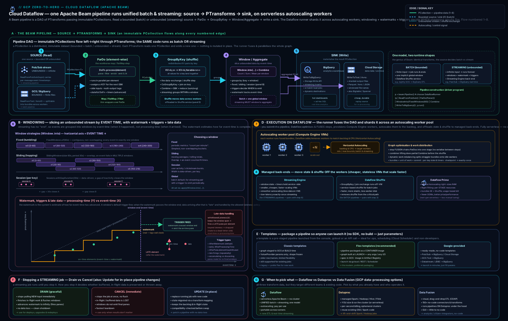
The diagram traces an unbounded stream from Pub/Sub through a Beam pipeline — ParDo → window assignment → GroupByKey/Combine → BigQuery sink — with the five streaming knobs off to the side: event-time windows as the buckets, the advancing watermark drawing the on-time/late line, the trigger emitting early/on-time/late panes, allowed lateness holding a window open for stragglers, and accumulation mode deciding whether each pane replaces or adds to the last; below it sits the execution layer — an autoscaling worker fleet with Streaming Engine holding state and shuffle in the service backend.
Going deeper
The serverless facade hides a lot of machinery. Knowing what actually happens after you press run — how Dataflow deduplicates, how it decides parallelism, how it computes the watermark, and how it bills — is exactly the depth the Professional Data Engineer exam and a serious streaming interview probe. This section is for the reader who already understood everything above.
Exactly-once processing — and where it stops being exactly-once
Dataflow gives exactly-once processing for the pipeline’s internal state: every input element affects each aggregation exactly once, even when workers crash, bundles retry, and the fleet rescales. It achieves this by checkpointing progress and by deduplicating on the shuffle using deterministic per-element identifiers — when a bundle is retried, records that already updated downstream state are recognised and dropped rather than double-counted. Streaming Engine (below) is where most of this checkpoint/dedup machinery lives.
The nuance that trips people up: exactly-once processing is not exactly-once side effects. Three honest caveats:
- Source dedup. Pub/Sub delivery is at-least-once — the same message can be redelivered. Dataflow deduplicates Pub/Sub messages using the message ID (or a payload attribute you nominate via
id_label/idAttribute) within a bounded window, so duplicate deliveries do not become duplicate records. Nominate a business idempotency key when the same event could be published twice, because Pub/Sub only dedups its own redeliveries, not your producer’s. - Sink side effects. A DoFn that calls an external API, sends an email, or does a naive HTTP
POSTcan run more than once on retry — Beam guarantees the element is processed exactly once into pipeline state, not that your side effect fires once. End-to-end exactly-once therefore needs an idempotent or transactional sink: BigQuery’s Storage Write API (exactly-once), or a write keyed so retries upsert the same row. External writes that cannot be made idempotent are the one place “exactly-once” leaks. - Non-determinism. If a DoFn produces different output on re-execution (it uses
random, wall-clock time, or a mutable global), the dedup keyed on its output cannot be trusted and results can drift. When a step must have a stable input before a side effect, annotate it@RequiresStableInput(Java) so Beam checkpoints first and any retry replays identical input.
Finally, you can trade exactly-once for latency and cost: Dataflow offers an at-least-once streaming mode (--dataflow_service_options=streaming_mode_at_least_once) that drops the dedup/checkpoint overhead. Use it only when the sink is already idempotent — it is cheaper and lower-latency, but records can appear more than once downstream. The default streaming mode is exactly-once.
Fusion, and when to break it
Dataflow fuses consecutive transforms into a single execution stage so the intermediate PCollection between them is never materialised or shuffled — a large, silent optimisation that avoids serialising data between a Map and a Filter. Usually fusion is pure win.
It bites in exactly one situation: a high-fan-out step. Suppose a ParDo reads 8 manifest files and each expands to ~2 million records. Because the ParDo is fused to its input’s parallelism (8-way), the whole 16-million-record expansion runs on ~8 workers and the fleet cannot scale, no matter how high --max_num_workers is — the parallelism is capped upstream. The symptom is a job that will not autoscale and a stage stuck at low parallelism.
The fix is a fusion break: insert a step that forces a materialise-and-shuffle so Dataflow can redistribute the expanded elements across the whole fleet. The idiomatic one is beam.Reshuffle() (Python) / Reshuffle.viaRandomKey() (Java); a GroupByKey or GroupIntoBatches breaks fusion too. Reshuffle doubles as a checkpoint — it prevents re-execution of expensive upstream work on retry — which is why it also appears before costly, non-idempotent steps.
Watermarks, holds, and the state-and-timers layer underneath
The watermark is computed per stage and only moves forward. A stage’s output watermark is bounded by the minimum of its input watermark and any watermark holds — a stage that has buffered an element it still intends to emit at an earlier timestamp holds the watermark back so it does not falsely declare that time complete. The Dataflow UI shows both a data watermark (event-time progress) and a system watermark; a stuck data watermark means windows are not closing.
Underneath windowing and triggers sits Beam’s state and timers API — the low-level primitive you reach for when the built-in windows and triggers do not fit. Within a stateful DoFn you get per-key-and-window state cells (ValueState, BagState, CombiningState, MapState) and timers you set in event time or processing time (@TimerId). Sessions, custom “emit after N or after T” logic, per-key deduplication, and rate-limiting are all expressible directly with state + timers. Watermark holds are what let a stateful DoFn buffer data and still emit it at the correct (earlier) event-time timestamp. This is advanced Beam, but it is the mechanism the high-level constructs are built on.
Hot keys and skew
A hot key — one key carrying a wildly disproportionate share of elements — serialises the GroupByKey/Combine for that key onto a single worker. The rest of the fleet idles, the watermark for that stage stalls, and autoscaling cannot help (adding workers does not split one key). It is the single most common cause of a stuck streaming pipeline.
Diagnose it by turning on hot-key logging (--experiments=enable_hot_key_logging, which surfaces the offending key value in the logs) and by watching for a large gap between average and max per-key work in a stage. Fixes depend on the aggregation:
- Combine (sum/mean/count): use
.with_hot_key_fanout(n)(Python) /.withHotKeyFanout(n)(Java). Because Combine is associative, Dataflow can split the hot key into n sub-keys, combine each partial in parallel, then combine the n partials — near-free correctness. - GroupByKey (you need the raw values): salt the key — append a random bucket suffix, group, then re-group on the real key — or pre-aggregate before the group. Also watch sliding windows, which multiply per-key state by
size/periodand amplify any skew.
Beam SQL (and why “Dataflow SQL” is gone)
You can express transforms in SQL inside a pipeline with Beam SQL: SqlTransform.query("SELECT ...") (Java) or the SqlTransform in apache_beam.transforms.sql (Python, via the Java expansion service on Runner v2). It supports streaming windows through table-valued functions — TUMBLE, HOP, and SESSION — so a windowed aggregation can be a SQL statement instead of a WindowInto + Combine. Beam SQL runs on Dataflow like any other transform.
Note the history so you do not chase a dead surface: the standalone “Dataflow SQL” offering — writing a SQL statement in the BigQuery UI or via gcloud dataflow sql query that launched a streaming Dataflow job directly — has been deprecated and retired. Do not build new work on it. For SQL over a stream today, use Beam SQL in a pipeline, a Google-provided template, or BigQuery’s own continuous queries — not the old Dataflow SQL command.
Autoscaling, Streaming Engine (Windmill), and Prime internals
Streaming autoscaling targets keeping the backlog small: Dataflow estimates backlog in seconds (how long the current queue would take to clear at the present throughput), watches CPU, and adjusts the worker count to hold backlog under a threshold — bounded by --max_num_workers, with dampening so it does not thrash, and with downscaling deliberately slower than upscaling (it is cheaper to be briefly over-provisioned than to flap). This only works well because Streaming Engine holds per-key state, timers, and the shuffle in the service backend (internally Windmill); a worker becomes nearly stateless, so Dataflow can add or remove one without moving gigabytes of state between VMs. That is the mechanistic reason Streaming Engine is effectively required for smooth streaming autoscaling. Batch autoscaling instead estimates remaining work and available parallelism, and Dataflow Shuffle likewise moves the batch shuffle to the backend.
Dataflow Prime adds two things on top. Vertical autoscaling watches memory pressure and OOM signals and replaces workers with higher-memory machines mid-job, so you never pre-size the whole fleet for its hungriest stage. Right Fitting attaches per-step resource hints (min_ram, accelerator) so one heavy or GPU stage gets a big machine while the rest stay small. Prime meters everything as Data Compute Units (DCUs) — one bundled unit spanning vCPU, memory, and Streaming Engine — instead of separate line items.
The cost model, dimension by dimension
Dataflow bills per second across several dimensions. Knowing which one dominates tells you what to optimise.
| Dimension | Charged on | Dominates when |
|---|---|---|
| vCPU | per vCPU-hour of running workers | Long-running streaming jobs (a worker is always up) |
| Memory | per GB-hour of worker RAM | Memory-heavy DoFns / large machines |
| Persistent Disk | per GB-hour | Jobs not on Streaming Engine/Shuffle (which slash local disk) |
| GPU | per accelerator-hour | ML inference inside the pipeline |
| Streaming Engine | data processed (streaming) | High-throughput streams — a separate charge from the workers |
| Dataflow Shuffle | data shuffled (batch) | Batch jobs with large joins/GroupByKey |
| Dataflow Prime | DCUs (bundles the above) | Prime-enabled jobs |
Two rules follow. In streaming, cost is dominated by time — a forgotten 24×7 job is the classic surprise bill, so cap it with --max_num_workers and stop it when idle. In batch, cost is dominated by data shuffled and vCPU-hours — prefer Combine over GroupByKey (less shuffle), and use FlexRS (--flexrs_goal=COST_OPTIMIZED) for delay-tolerant batch to run on discounted mixed preemptible/regular VMs scheduled within ~6 hours.
Update compatibility and version caveats
--update maps the new job’s transform graph onto the running one by step name, then carries over state and the in-flight watermark. What is compatible vs not:
- Compatible (accepted): adding new steps, changing a DoFn’s business logic that does not change its state or output coder, editing non-stateful internals.
- Incompatible (rejected): renaming a stateful step (bridge it with
--transform_name_mapping='{"old":"new"}'), changing a step’s coder or a window/trigger in a way that changes the state layout, or a fusion change that moves state. When rejected, you drain and relaunch (accepting a brief gap) — or, if the sink is idempotent, run old and new in parallel briefly.
Version caveats worth carrying: Runner v2 (the Docker-based portability framework) is the default and is required for Python streaming and cross-language transforms. Beam SDK versions have a support window — very old SDKs are eventually deprecated on Dataflow, so stay within the supported range. And the DirectRunner is local-testing only: it deliberately runs extra correctness checks (element immutability, coder round-tripping, out-of-order delivery) that the DataflowRunner does not, precisely to surface bugs before you spend on the cloud.
Hands-on lab
This lab runs the canonical streaming pipeline — Pub/Sub → Dataflow → BigQuery — using a Google-provided Flex template (so you do not need the SDK installed), watches it autoscale, then drains it cleanly. It runs for a few minutes and costs cents on the $300 credit. Set your project first.
export PROJECT=$(gcloud config get-value project)
export REGION=us-central1
export BUCKET=gs://${PROJECT}-dataflow-lab
gcloud services enable dataflow.googleapis.com compute.googleapis.com \
  pubsub.googleapis.com bigquery.googleapis.com storage.googleapis.com
1. Create the staging bucket, a Pub/Sub topic + subscription, and a BigQuery dataset/table.
gsutil mb -l $REGION $BUCKET
gcloud pubsub topics create lab-events
gcloud pubsub subscriptions create lab-events-sub --topic=lab-events
bq mk --dataset --location=$REGION ${PROJECT}:dataflow_lab
bq mk --table ${PROJECT}:dataflow_lab.events \
  'data:STRING,attributes:STRING,message_id:STRING,publish_time:TIMESTAMP'
2. Launch the Google-provided “Pub/Sub Subscription to BigQuery” Flex template. No code — just parameters.
gcloud dataflow flex-template run "lab-ps-to-bq-$(date +%s)" \
  --template-file-gcs-location=gs://dataflow-templates-${REGION}/latest/flex/PubSub_Subscription_to_BigQuery \
  --region=$REGION \
  --parameters=inputSubscription=projects/${PROJECT}/subscriptions/lab-events-sub,outputTableSpec=${PROJECT}:dataflow_lab.events \
  --temp-location=${BUCKET}/temp \
  --max-workers=3 \
  --enable-streaming-engine
Expected output: a job resource with an id and currentState: JOB_STATE_QUEUED → JOB_STATE_RUNNING. The job appears in the Dataflow → Jobs console with a live execution graph.
3. Publish some events so there is data to flow through.
for i in $(seq 1 20); do
  gcloud pubsub topics publish lab-events \
    --message="{\"event\":\"click\",\"n\":$i}" \
    --attribute=source=lab
done
4. Watch it run and autoscale. List the job, then inspect it.
gcloud dataflow jobs list --region=$REGION --status=active
JOB_ID=$(gcloud dataflow jobs list --region=$REGION --status=active \
  --format='value(JOB_ID)' --filter="NAME:lab-ps-to-bq" | head -1)
gcloud dataflow jobs describe $JOB_ID --region=$REGION
In the console, open the job and watch the execution graph, the data watermark per stage, and the autoscaling panel (worker count over time). Within a minute or two you should see workers spin up.
5. Validate the data landed in BigQuery.
bq query --use_legacy_sql=false \
  "SELECT COUNT(*) AS rows FROM \`${PROJECT}.dataflow_lab.events\`"
Expected output: a non-zero rows count matching the messages you published (allow a minute for the pipeline to process and write).
6. Drain the streaming job (graceful stop — flushes in-flight data, then shuts down). Contrast with cancel, which would stop immediately.
gcloud dataflow jobs drain $JOB_ID --region=$REGION
# (use `gcloud dataflow jobs cancel $JOB_ID --region=$REGION` to stop *now* and discard in-flight data)
gcloud dataflow jobs list --region=$REGION   # state moves to JOB_STATE_DRAINING → JOB_STATE_DRAINED
Cleanup (do this — a running streaming job bills continuously, which is the one way this lab could cost real money):
# ensure the job is stopped (drained/cancelled) first, then:
bq rm -r -f -d ${PROJECT}:dataflow_lab
gcloud pubsub subscriptions delete lab-events-sub
gcloud pubsub topics delete lab-events
gsutil -m rm -r $BUCKET
Cost note: the only meaningful charge is the workers running while the streaming job is up — a couple of small workers for a few minutes is cents, fully absorbed by the $300 credit. Streaming Engine adds a small data-processed charge. The expensive mistake is forgetting to drain/cancel a streaming job — it will run (and bill) 24×7 until you stop it. Pub/Sub (10 GiB/month free), this volume of BigQuery storage/writes, and the GCS staging are all effectively free at lab scale. Always confirm gcloud dataflow jobs list --status=active is empty when you are done.
Practice challenges
Work these in order — they escalate from beginner to advanced. Try each before opening the solution. No live runtime is assumed; every command and snippet is real and schema-correct, so you can run them in your own project. Replace placeholders (PROJECT, REGION, JOB_ID, SUB) with your own values.
Challenge 1 (beginner) — Launch the textbook pipeline with no code. Enable the Dataflow stack, then launch the Google-provided “Pub/Sub Subscription to BigQuery” Flex template into an existing subscription lab-events-sub and table dataflow_lab.events, with Streaming Engine and a 3-worker cap.
<details> <summary>Solution</summary>
gcloud services enable dataflow.googleapis.com pubsub.googleapis.com \
  bigquery.googleapis.com compute.googleapis.com

gcloud dataflow flex-template run "ps-to-bq-$(date +%s)" \
  --template-file-gcs-location=gs://dataflow-templates-${REGION}/latest/flex/PubSub_Subscription_to_BigQuery \
  --region=$REGION \
  --parameters=inputSubscription=projects/${PROJECT}/subscriptions/lab-events-sub,outputTableSpec=${PROJECT}:dataflow_lab.events \
  --temp-location=gs://${PROJECT}-dataflow-lab/temp \
  --max-workers=3 --enable-streaming-engine
Why: Google-provided templates run the common pipelines with no SDK and no source — you supply parameters, Dataflow builds and runs the Beam graph. </details>
Challenge 2 (beginner) — Stop a streaming job the graceful way. You have a running streaming JOB_ID. Stop it so in-flight data is flushed and open windows close, and state (in one line) which command you would use instead to stop now and discard in-flight data.
<details> <summary>Solution</summary>
gcloud dataflow jobs drain $JOB_ID --region=$REGION
# stop-now-and-discard alternative:
gcloud dataflow jobs cancel $JOB_ID --region=$REGION
Why: drain advances the watermark to infinity so every open window flushes before shutdown (no in-flight loss); cancel is immediate and lossy. Reach for drain by default. </details>
Challenge 3 (intermediate) — Window and trigger a Pub/Sub stream in Beam (Python). Write the pipeline fragment that reads Pub/Sub taking event time from a message attribute event_time, applies a 60-second fixed window, and a trigger that fires early every 10 s, on time at the watermark, and late for up to 10 minutes of allowed lateness, in accumulating mode.
<details> <summary>Solution</summary>
import apache_beam as beam
from apache_beam.transforms.window import FixedWindows
from apache_beam.transforms.trigger import (
    AfterWatermark, AfterProcessingTime, AccumulationMode)

windowed = (
    pcoll
    | "Read" >> beam.io.ReadFromPubSub(
          subscription=SUB, timestamp_attribute="event_time")
    | "Window" >> beam.WindowInto(
          FixedWindows(60),
          trigger=AfterWatermark(
              early=AfterProcessingTime(10),   # speculative every 10 s
              late=AfterProcessingTime(10)),   # re-fire as late data lands
          allowed_lateness=600,                # 10 minutes, in seconds
          accumulation_mode=AccumulationMode.ACCUMULATING))
Why: window = the bucket, trigger = when/how often to emit, allowed lateness = how long to keep the window open for stragglers, accumulating = each pane replaces the last (pair it with an upsert sink). </details>
Challenge 4 (intermediate) — Match the accumulation mode to the sink. A windowed Combine counts events per minute; the BigQuery sink INSERTs each pane as a new row and a dashboard SUMs them. On-time plus late panes for the same window are double-counting the total. Give two correct fixes.
<details> <summary>Solution</summary>
Fix A — change the mode to match the additive sink:
accumulation_mode=AccumulationMode.DISCARDING # each pane = only new elements
Fix B — keep ACCUMULATING and make the sink upsert/overwrite the window’s row (key the BigQuery row by window start), so each pane replaces the previous best answer instead of adding to it.
Why: accumulating + additive sink = inflated totals. Either emit deltas (discarding) into an additive sink, or emit the running total (accumulating) into an overwrite sink — never mix. </details>
Challenge 5 (advanced) — Break fusion for a high-fan-out step. A batch pipeline’s ParDo reads 8 GCS manifest files and each expands to ~2 million records, but only ~8 workers ever run and the job will not autoscale past that. Explain why, and fix it with one transform.
<details> <summary>Solution</summary>
records = (
    manifests                              # 8 elements → 8-way parallelism
    | "Expand" >> beam.ParDo(ExpandManifest())   # fused to the 8-way input
    | "Break fusion" >> beam.Reshuffle()          # materialise + shuffle
    | "Heavy" >> beam.ParDo(ExpensiveStep()))     # now scales across the fleet
Why: fusion pins the expansion to the input’s 8-way parallelism, so --max_num_workers can’t help. beam.Reshuffle() forces a materialise-and-shuffle, redistributing the ~16 M expanded records across the whole fleet (and checkpointing the expensive upstream work).
</details>
Challenge 6 (advanced) — Deploy a fix to a 24×7 job without losing state, and know when you can’t. You changed a DoFn’s business logic (no state or coder change) on a stateful streaming job. Deploy it with no data loss and no replay, then name the one change that would force a drain-and-relaunch instead.
<details> <summary>Solution</summary>
Relaunch the same pipeline with the same job name and --update:
python my_pipeline.py --runner=DataflowRunner --region=$REGION \
  --job_name=my-streaming-job --update \
  --temp_location=gs://${PROJECT}-dataflow-lab/temp
# (bridge a renamed step with --transform_name_mapping='{"OldName":"NewName"}')
Incompatible change → drain then relaunch: renaming a stateful step or changing its coder / window layout changes the state shape, which --update cannot map.
Why: --update matches steps by name and carries state + the in-flight watermark across; only edits that change the state layout are rejected.
</details>
Common beginner mistakes
These are misconceptions — the wrong mental model that produces the wrong instinct — not error messages. (For symptom → cause → fix, see the troubleshooting table below.)
- “Streaming and batch need two different pipelines.” They don’t: one Beam pipeline serves both. Right model — write the transforms once; batch vs streaming is a difference in the data shape (bounded vs unbounded source) and the windowing, not a rewrite.
- “The window decides when I get results.” No — the window is only which bucket an element lands in. Right model — the trigger decides when/how often to emit, the watermark decides when the input is complete, and allowed lateness decides how long to wait for stragglers. Four separate knobs; the window is just one.
- “Pub/Sub publish time is my event time.” Publish time drifts by the ingestion delay. Right model — take the timestamp from the true event field in the payload (
timestamp_attribute/outputWithTimestamp), or your windows are shifted by however long the data took to arrive. - “Late data just works.” Allowed lateness defaults to zero, so late events are dropped silently — no error. Right model — to keep stragglers you must set
withAllowedLateness(...)and a late-firing trigger, and choose an accumulation mode. - “I control the workers / one worker per key.” You don’t hand-place workers — Dataflow autoscales. Right model — you set a ceiling (
--max_num_workers), not a fixed fleet, and one hot key can bottleneck the whole job no matter how many workers you allow. - “GroupByKey is how you sum.” It works but shuffles every raw value. Right model — prefer Combine for sums/means/counts: it partial-combines on each worker before the shuffle, moving far less data.
- “Cancel is just a clean stop.” Cancel discards in-flight data. Right model — drain is the clean stop that flushes in-flight data and closes open windows; reach for drain unless the job is wedged.
- “Exactly-once means my HTTP POST fires once.” Exactly-once covers pipeline state, not external side effects; a bundle can retry. Right model — make external writes idempotent (or use a transactional sink like the Storage Write API), or a retried DoFn will repeat the side effect.
- “I’ll just leave the streaming job running.” A streaming job bills continuously, 24×7 — the classic surprise bill is a forgotten job. Right model — drain it when you’re done, and confirm
gcloud dataflow jobs list --status=activeis empty.
Common mistakes & troubleshooting
| Symptom | Likely cause | Fix |
|---|---|---|
| Streaming job never emits results | Default global window kept in streaming with the default trigger (never fires); or watermark stuck | Apply an event-time window (fixed/sliding/session), or add an explicit trigger to the global window; investigate the stuck stage |
| Late events silently missing from windows | Allowed lateness defaults to zero — late data is dropped | Set withAllowedLateness(...) and an AfterWatermark.withLateFirings() trigger; pick an accumulation mode |
| Watermark stuck / lagging far behind | A slow/oversubscribed stage, hot key (one key with disproportionate data), or too few workers | Raise --max_num_workers, fix the hot key (add salt / better key), enable Streaming Engine; check the per-stage watermark in the UI |
| Double-counted totals in the sink | ACCUMULATING mode into an additive sink (or late panes re-added) |
Use DISCARDING for additive sinks, or ACCUMULATING with an upsert/overwrite sink keyed by window |
Job stuck QUEUED / fails to start |
Worker SA lacks roles/dataflow.worker or source/sink access; bad --temp_location; quota for CPUs exhausted |
Grant the worker SA correct roles + I/O access; supply a valid GCS temp path; check Compute Engine CPU quota in the region |
| Update rejected (“incompatible”) | Renamed a stateful step, or changed a window/coder incompatibly | Provide a --transform_name_mapping, keep stateful step names stable, or drain then relaunch for incompatible changes |
| Wrong-time windows (events in the wrong bucket) | Timestamp taken from Pub/Sub publish time instead of the true event time in the payload | Set the element timestamp from the payload’s event time (timestamp_attribute / outputWithTimestamp) |
| OutOfMemory on workers | Memory-heavy DoFn / large per-key state on too-small a machine | Use a bigger --worker_machine_type, fewer harness threads, or Dataflow Prime vertical autoscaling; reduce per-key state |
| Sliding-window job is huge/expensive | Tiny period over a large size → each element in many windows |
Increase the period or reduce the size; reconsider whether you need a sliding window |
| Streaming autoscaling not happening | Streaming Engine not enabled | Add --enable_streaming_engine (required for responsive streaming autoscaling) |
Best practices
- Always window your streaming data in event time and choose the trigger/lateness/accumulation triplet deliberately — these five knobs (window, watermark, trigger, allowed lateness, accumulation mode) are the whole game.
- Use the true event time from the payload, not Pub/Sub publish time, so windows are correct regardless of ingestion delay.
- Enable Streaming Engine for every streaming job (smoother autoscaling, smaller/cheaper workers, less disk) and rely on Dataflow Shuffle for batch (it is the default).
- Prefer Combine over GroupByKey whenever you only need an aggregate — partial combining before the shuffle is dramatically cheaper than grouping all raw values.
- Cap cost with
--max_num_workersand let autoscaling handle the rest; never hard-pin a large fixed fleet “to be safe”. - Write to BigQuery with the Storage Write API (exactly-once, cheaper than legacy streaming inserts) and use
FILE_LOADSfor pure batch. - Ship reusable pipelines as Flex templates, and check the Google-provided catalogue first — the common pipelines (Pub/Sub→BQ, GCS→BQ, etc.) are already built.
- Use
--updateto deploy changes to 24×7 streaming jobs so you keep state; keep stateful step names stable to preserve update compatibility. - Drain (not cancel) for graceful stops so in-flight data is flushed; cancel only when you must stop immediately.
- Run workers with a least-privilege service account on private IPs (
--no_use_public_ips+ Cloud NAT / Private Google Access). - Test locally with the DirectRunner before spending on Dataflow, and write unit tests with Beam’s
TestPipeline/PAssert.
Security notes
- Two identities matter. The submitter needs
roles/dataflow.developerandiam.serviceAccounts.actAson the worker SA; the workers run as a worker service account that must haveroles/dataflow.workerplus only the read/write roles for the specific sources and sinks (e.g.pubsub.subscriber,bigquery.dataEditor). Do not run workers as the default Compute Engine service account with broad scopes — create a dedicated, least-privilege SA with--service_account_email. - Keep workers off the public internet with
--no_use_public_ipsand a--subnetwork; provide egress via Cloud NAT and reach Google APIs via Private Google Access. - Encrypt job state and temp data with CMEK using
--dataflow_kms_keywhere compliance requires customer-managed keys (the Dataflow service agent needs encrypt/decrypt on the key). - Scope source/sink access tightly — a pipeline that only reads one subscription and writes one table should have exactly those two grants, nothing wider.
- Use VPC Service Controls to put Dataflow, Pub/Sub, BigQuery, and GCS inside a perimeter so data cannot be exfiltrated to projects outside it.
- Audit Logs (Admin Activity always on; enable Data Access logs) record who launched, drained, or cancelled jobs — wire them into your central sink.
- Mind staging buckets: your pipeline code and temp data live in
--staging_location/--temp_location— lock those buckets down; they can contain sensitive logic and intermediate data.
Interview & exam questions
1. Explain the difference between event time and processing time, and why it matters. Event time is when the event actually happened (the timestamp in the data); processing time is when the pipeline observed it (worker wall clock). They diverge by skew (network delay, queueing, offline devices). Windowing is defined in event time so aggregates are correct regardless of arrival delay; the watermark bridges the two by estimating event-time progress.
2. What is a watermark, and what does it decide? Dataflow’s continuously updated estimate that “event time has reached T and I have seen (almost) all events ≤ T.” When it passes a window’s end, the window’s input is considered complete and (with the default trigger) the on-time result is emitted. It is heuristic, so some events arrive after it — those are late.
3. Describe the four window types and a use case for each.
Fixed/tumbling — contiguous non-overlapping intervals (“per-minute counts”). Sliding/hopping — overlapping fixed-length windows advancing by a period (“trailing 1-min average every 10 s”; each element in size/period windows). Session — data-driven, per-key, variable length closed by an inactivity gap (“a user session”). Global — one window for all time (batch totals; streaming only with an explicit trigger).
4. By default, what happens to late data, and how do you incorporate it?
By default allowed lateness is zero, so late data (arriving after the watermark passes its window) is dropped. To include it, set withAllowedLateness(duration) and a late-firing trigger (AfterWatermark.withLateFirings(...)), and choose an accumulation mode. More allowed lateness = more state held = more cost.
5. Accumulating vs discarding accumulation mode — when each? Accumulating: each pane re-emits the full result so far — use with an upsert/overwrite sink keyed by window. Discarding: each pane emits only the new elements since the last firing — use with an additive sink. Mismatch causes double-counting (accumulating + additive) or lost data (discarding + overwrite).
6. Drain vs cancel vs update.
Drain (streaming): stop ingesting, finish in-flight work, advance the watermark so windows flush, then stop — graceful, no in-flight loss (but late data after the drain is lost). Cancel: stop immediately, discard in-flight data — fast, lossy. Update (--update): replace a running streaming job with new code while preserving state and watermark — for zero-downtime deploys; requires a compatible graph (stateful step names/types must match).
7. What does Streaming Engine do, and why does it matter for autoscaling? It moves the streaming pipeline’s state and shuffle off worker VMs into the Dataflow service backend. Workers become small and disposable, so autoscaling can rebalance smoothly and quickly (no need to move large state between VMs) and disks shrink. It is effectively required for responsive streaming autoscaling and is the default for new streaming jobs.
8. GroupByKey vs Combine — why prefer Combine? Both aggregate by key, but Combine is associative/commutative, so Dataflow does partial combining on each worker before the shuffle (e.g. local partial sums), moving far less data across the network. GroupByKey shuffles all raw values to one place. For sums/means/counts, Combine is dramatically cheaper.
9. How do you run a pipeline without the SDK, with runtime parameters? Classic vs Flex templates?
Use a template. Classic: graph staged to GCS at build time; only ValueProvider params vary (legacy). Flex: pipeline packaged as a Docker image + spec in GCS, graph built at launch so any param can vary and you can bake in dependencies — the recommended approach. Or use a Google-provided template (Pub/Sub→BQ, GCS→BQ, etc.) for the common cases.
10. Dataflow vs Dataproc vs Cloud Data Fusion? Dataflow: serverless Apache Beam, unified batch+streaming, lowest ops — choose for green-field pipelines. Dataproc: managed Spark/Hadoop clusters — choose to lift-and-shift existing Spark/Hadoop or when you need a specific OSS engine. Cloud Data Fusion: visual no-code ETL (runs on Dataproc) — choose for non-engineers building drag-and-drop pipelines.
11. Your streaming job’s watermark is stuck and results stopped appearing. How do you diagnose it?
Open the per-stage watermark in the Dataflow UI to find the lagging stage; check the backlog and CPU; look for a hot key (skew), an under-provisioned fleet (raise --max_num_workers), Streaming Engine not enabled, or a slow external call in a DoFn. A stuck watermark means windows cannot close.
12. Why might windows contain events from the wrong time, and how do you fix it?
Because the element timestamp was taken from Pub/Sub publish time (or assigned at processing time) rather than the true event time in the payload, so ingestion delay shifts events into later windows. Fix by setting the timestamp from the payload’s event-time field (timestamp_attribute on the Pub/Sub read, or outputWithTimestamp in a DoFn).
13. What is Dataflow Prime and when would you use it? The next-gen execution platform adding vertical autoscaling (auto-adjusting worker memory, not just count) and Right Fitting (per-stage resource hints), billed in DCUs. Use it for jobs with variable or hard-to-predict resource needs (uneven memory, a single hungry stage) so you do not size the whole job for its worst step.
14. What exactly does “exactly-once” cover in Dataflow, and where does it not hold? It covers pipeline state — each element affects each aggregation once despite retries and rescaling, via checkpointing and shuffle-based dedup. It does not cover external side effects: a DoFn calling an API or doing an HTTP POST can run more than once on retry, so external writes must be idempotent (or transactional, like the Storage Write API). Non-deterministic DoFns can also break the guarantee unless you force stable input.
15. What is fusion, and when do you deliberately break it?
Fusion merges adjacent transforms into one stage so intermediate data is never materialised — usually a win. You break it for a high-fan-out step, where the expansion is pinned to the (small) input’s parallelism and the fleet can’t scale; inserting beam.Reshuffle() (or a GroupByKey) forces a shuffle so downstream work redistributes across all workers.
Quick check
- Which window type is data-driven, per-key, and closed by an inactivity gap?
- What is the default allowed lateness, and what does that imply for late events?
- Which Dataflow feature moves streaming state and shuffle into the service backend, and what does it enable?
- Which stop operation preserves in-flight data by flushing it before shutting down — drain or cancel?
- To deploy new code to a 24×7 streaming job without losing state, which operation do you use?
- “Exactly-once” in Dataflow guarantees each element affects pipeline state once — what does it not guarantee?
Answers
- Session windows.
- Zero — by default late events (arriving after the watermark passes their window) are dropped; you must set
withAllowedLatenessand a late trigger to keep them. - Streaming Engine — it enables smooth, responsive streaming autoscaling (and smaller workers/disks).
- Drain (cancel stops immediately and discards in-flight data).
- Update (
--update/gcloud dataflow jobs update), with a compatible transform graph. - External side effects — a DoFn’s outward writes/API calls can repeat on retry, so sinks must be idempotent or transactional for end-to-end exactly-once.
Exercise
Build the classic streaming-analytics pipeline end to end and exercise the time machinery. Create a Pub/Sub topic taxi-rides and a subscription, and a BigQuery table for per-minute aggregates. Write (or adapt a Beam quickstart for) a streaming pipeline that: reads from the subscription using a payload event-time field as the element timestamp (not publish time); applies a fixed 60-second event-time window; uses a trigger that fires early every 10 seconds (speculative), on time at the watermark, and late for up to 10 minutes of allowed lateness, in accumulating mode; Combines to count rides per window; and writes to BigQuery via the Storage Write API keyed so that accumulating panes upsert (overwrite) the window’s row. Launch it on Dataflow with Streaming Engine, --max_num_workers=4, a least-privilege worker service account, and no public IPs. Publish a burst of events including two deliberately late ones (timestamps a few minutes in the past) and confirm: on-time panes appear within a window, the late panes update the affected window’s row (not double-counted, because accumulating + upsert), and the autoscaling panel shows the fleet sizing to the load. Then make a compatible code change (e.g. add a field) and deploy it with --update, confirming the job keeps running with no data loss. Finally drain the job and verify the final windows flush. Tear everything down. Note which changes would have made the update incompatible and forced a drain-then-relaunch.
Certification mapping
- Associate Cloud Engineer (ACE): know that Dataflow is the serverless service for running Apache Beam batch and streaming pipelines, how to launch a Google-provided template with
gcloud dataflow flex-template run, the basics of autoscaling and worker options, and how to drain/cancel a streaming job. Recognise the canonical Pub/Sub → Dataflow → BigQuery pattern. - Professional Data Engineer (PDE): the heavyweight exam here. Expect deep scenario questions on windowing (fixed/sliding/session — pick the right one), event time vs processing time, watermarks, triggers (early/on-time/late, allowed lateness, accumulating vs discarding), exactly-once with the Storage Write API, drain vs cancel vs update, Streaming Engine / Shuffle / Prime, autoscaling and cost control, classic vs Flex templates, and the Dataflow vs Dataproc vs Cloud Data Fusion decision. Hot keys, late-data handling, and reprocessing/replay are common distractor-rich questions.
- Professional Cloud Architect (PCA): Dataflow as the processing layer in event-driven and analytics architectures (Pub/Sub → Dataflow → BigQuery/Bigtable), choosing it versus Dataproc/Data Fusion, and the operational story (serverless, autoscaling, zero-downtime updates) plus data-residency via region/CMEK/VPC-SC.
Glossary
- Apache Beam — the open-source, portable programming model and SDK (Java/Python/Go) for batch+streaming pipelines that Dataflow runs.
- Pipeline — the whole DAG of transforms from source(s) to sink(s); run with the DirectRunner (test) or DataflowRunner (prod).
- PCollection — Beam’s distributed, immutable dataset between transforms; bounded (batch) or unbounded (streaming).
- PTransform — an operation on PCollections (map, filter, window, group, read, write); composable.
- ParDo / DoFn — the general per-element transform; the DoFn’s
processmethod emits 0…N outputs per input. - GroupByKey — groups values by key (requires a shuffle); forces windowing/triggers in streaming.
- Combine — associative/commutative aggregation (sum/mean/count) with partial combining before the shuffle — cheaper than GroupByKey.
- CoGroupByKey / Flatten / side input — relational join of keyed PCollections / union of same-type PCollections / small broadcast lookup view.
- Bounded vs unbounded — finite (batch) vs infinite (streaming) PCollection.
- Event time vs processing time — when the event happened (in the data) vs when the pipeline saw it (worker clock).
- Window — an event-time bucket: fixed (tumbling), sliding (hopping, overlapping), session (gap-based, per-key), or global.
- Watermark — Dataflow’s estimate of event-time progress; when it passes a window’s end the window is “complete”.
- Watermark hold — a stage keeping the watermark from advancing past buffered data it still intends to emit at an earlier timestamp.
- Trigger — decides when/how often a window emits a result (pane):
AfterWatermark(on-time), early firings, late firings,AfterProcessingTime,AfterCount, composites. - Pane — one emission of a window’s result (early, on-time, or late).
- Allowed lateness — how long after the watermark a window’s state is kept so late data can update it (default zero = drop late data).
- Accumulation mode — accumulating (each pane = full result so far; for overwrite sinks) vs discarding (each pane = deltas; for additive sinks).
- State & timers — per-key-and-window state cells (Value/Bag/Combining/Map) plus event-/processing-time timers; the low-level primitive under windowing and triggers.
- Exactly-once processing — every element affects pipeline state once despite retries (via checkpointing + shuffle dedup); external side effects still need idempotence.
- At-least-once streaming mode — a Dataflow streaming mode (
streaming_mode_at_least_once) that drops dedup overhead for lower latency/cost when the sink is idempotent. - RequiresStableInput — an annotation forcing a checkpoint (stable input) before a side-effecting step so retries replay identical input.
- Autoscaling — Dataflow adjusting worker count on throughput (batch) or backlog (streaming); bounded by
--max_num_workers. - Streaming Engine — moves streaming state + shuffle into the service backend (internally Windmill) for smooth autoscaling and smaller workers/disks.
- Dataflow Shuffle — the batch equivalent: service-side shuffle off the workers (default for batch).
- Dataflow Prime — next-gen platform adding vertical autoscaling (memory) and Right Fitting (per-stage hints), billed in DCUs.
- Data Compute Unit (DCU) — Dataflow Prime’s single billing unit bundling vCPU, memory, and Streaming Engine.
- Fusion / fusion break — Dataflow’s optimisation that merges adjacent transforms to avoid materialising intermediate data; a fusion break (
beam.Reshuffle(), GroupByKey) forces a shuffle to restore parallelism after a high-fan-out step. - Hot key — a key holding a disproportionate share of data, serialising a GroupByKey/Combine; fixed with Combine
withHotKeyFanoutor by salting the key. - FlexRS — Flexible Resource Scheduling: discounted, delay-scheduled batch on mixed preemptible/regular VMs (
--flexrs_goal). - Beam SQL —
SqlTransformrunning SQL (withTUMBLE/HOP/SESSIONwindows) inside a Beam pipeline; the standalone “Dataflow SQL” surface is retired. - Classic / Flex / Google-provided template — staged-graph (legacy) / Docker-image (recommended) / ready-made templates to launch jobs without source code.
- Drain / cancel / update — graceful stop flushing in-flight data / immediate stop discarding it / in-place code swap preserving state.
- Runner v2 — Dataflow’s default Docker-based portability framework (required for Python streaming and cross-language transforms).
- Runner — the engine that executes a Beam pipeline (DataflowRunner, DirectRunner, Flink, Spark).
- Storage Write API — BigQuery’s modern, exactly-once, cost-efficient write path used by BigQueryIO.
Next steps
- Go upstream to the source with the Pub/Sub deep dive — topics, subscriptions, delivery guarantees, ordering, and dead-lettering that feed every streaming Dataflow job.
- Go downstream to the sink with the BigQuery deep dive — datasets, partitioning, the Storage Write API, and slots/pricing for the warehouse your pipeline writes to.
- Continue the course with the Identity-Aware Proxy deep dive to add zero-trust access to the apps and dashboards built on this data. </content> </invoke>