In a nutshell
Imagine the best shop assistant you have ever met. They remember what every one of your millions of customers has browsed and bought, they know every one of your 250,000 products cold, and when a shopper walks in they can instantly point to the handful of items that person is most likely to want next — in the time it takes the page to paint. That assistant is what a recommendation engine is: software that predicts, for this specific shopper right now, which products to put in the “Recommended for you” rail.
The clever bit is how it stays fast. You cannot have the assistant mentally compare the shopper against all 250,000 products on every visit — that is far too slow. So this design teaches the assistant two skills with the same mental yardstick. One skill reads a shopper and turns them into a point on a map (“this person, right now, wants budget-friendly baby and household items”). The other skill reads a product and turns it into a point on the same map. Because shoppers and products live on one shared map, recommending becomes simple: find the products sitting closest to the shopper’s point. That “two skills, one map” idea is the two-tower model, and “find the closest points fast” is vector search. A second, pickier assistant then puts the closest few hundred into the best final order — that is the ranking model.
This lesson is the engineering blueprint for building that engine on Google Cloud’s Vertex AI: how the two towers are trained, how vector search retrieves candidates in milliseconds, how features are kept fresh as a shopper fills their cart, how you handle brand-new products and brand-new shoppers, and — the part that funds the whole thing — how you prove with an A/B test that the new rail actually earns more money. It is deliberately the engine internals; the broader enterprise wrap (org design, ITSM, the full security stack) lives in a companion lesson.
Level: Intermediate · Time: ~36 min
Prerequisites & what you’ll be able to do. You’ll get the most from this if you’re comfortable with the idea of a machine-learning model as something you train on history and then serve predictions from, you know what an API request and response are, and you have seen BigQuery or another SQL warehouse. Deep math is not required — every idea is explained in plain language first. For the surrounding platform context, the Vertex AI Pipelines MLOps guide covers the training orchestration this engine plugs into, and the BigQuery deep dive covers the data layer it sits on. After working through this lesson you will be able to:
- Explain the two-stage funnel — candidate generation (retrieval) then ranking — and why real-time recommenders are built this way instead of scoring the whole catalog.
- Describe how a two-tower model produces user and item embeddings in a shared space, how it is trained, and how matrix factorization relates to it as a simpler baseline.
- Reason about Vector Search (ScaNN): approximate nearest-neighbour retrieval, filtering with restricts, and the recall-vs-latency dial you tune to hit a p99 budget.
- Keep features consistent and fresh with a Feature Store (batch materialization for training, streaming updates for in-session freshness) and avoid training/serving skew.
- Handle cold-start for new items and new users, and read offline evaluation metrics (recall@k, NDCG) without mistaking them for guaranteed revenue.
- Run an A/B test that produces a defensible lift number, and know when to reach for the managed alternative, Vertex AI Search for commerce, instead of building.
A national grocery and general-merchandise retailer — 1,400 stores, an app and web storefront doing 18 million sessions a week — gets a directive from its Chief Digital Officer after a brutal quarter: a discount-grocery competitor has been eating its margin, basket sizes are flat, and the “Recommended for you” rail on the homepage is a static, merchandiser-curated list that has not been personalized to a single shopper since it launched. The ask is specific: every logged-in customer should see a recommendation rail that reflects what they actually browse and buy, it should update within the same session when someone adds milk and bread to the cart, and the merchandising team must be able to prove — with a number the CFO trusts — that the new rail lifts revenue before it rolls out to all stores. The constraint is just as specific: this runs on GCP, the data platform is already BigQuery, peak is the 6pm weekday rush and the days before a holiday, and the security team will not approve anything that lets a third party touch customer purchase history. This article is the reference architecture for building that engine properly on Vertex AI — a two-tower retrieval model, a feature store, a streaming clickstream, a stateless serving tier, and an experimentation harness that a head of merchandising and a CISO will both sign.
The pressures stack the way they do in retail. Scale means tens of thousands of recommendation requests per second at the dinner-hour peak, against a catalog of 250,000 SKUs. Latency means the rail must render inside the page’s render budget — a recommendation that arrives after the homepage paints is a recommendation nobody sees, so the p99 budget is tens of milliseconds, not seconds. Freshness means in-session signal: the customer who just put nappies in the cart should see formula and wipes before they reach checkout, not tomorrow. And measurability means the engine is worthless to the business until an A/B test proves incremental revenue, because merchandising has been burned by “AI” that looked clever and moved no money. A two-tower retrieval model on Vertex AI satisfies all four, and the rest of this architecture exists to feed it, serve it, and prove it.
Why two-tower retrieval, not the obvious shortcuts
The naive approaches each fail predictably, and naming why matters because someone on the project will propose all three.
Hand-curated merchandiser rails — the status quo — do not personalize at all; they show the same “top sellers” to a vegan and a household of five, and they go stale the moment a promotion ends. A single “people who bought X also bought Y” co-occurrence table is better but brittle: it is recomputed in a nightly batch, has nothing to say about a brand-new SKU or a brand-new customer (the cold-start problem), and cannot fuse a shopper’s long-term taste with what they did ten seconds ago. A monolithic deep model that scores every one of 250,000 SKUs per request is mathematically the “right” answer and operationally impossible — scoring a quarter-million items inside a 40-millisecond budget at peak QPS is not something you can pay your way out of.
The two-tower architecture threads the needle, and it is worth understanding because it shapes everything downstream. You train two neural networks. The query tower ingests user and context features — recent browse and purchase history, time of day, store, device — and emits a single embedding vector representing “what this shopper wants right now.” The candidate tower ingests item features — category, brand, price band, attributes — and emits an embedding for each SKU. The training objective pulls the embeddings of items a user actually engaged with close to that user’s embedding, and pushes everything else away. The payoff is the operational trick: because items and users live in the same vector space, serving a recommendation becomes an approximate nearest-neighbor (ANN) lookup — embed the user once, find the closest item vectors in single-digit milliseconds, and never score 250,000 items at request time. Retrieval narrows a quarter-million SKUs to a few hundred candidates; a cheaper ranking pass then orders that shortlist.
Architecture overview
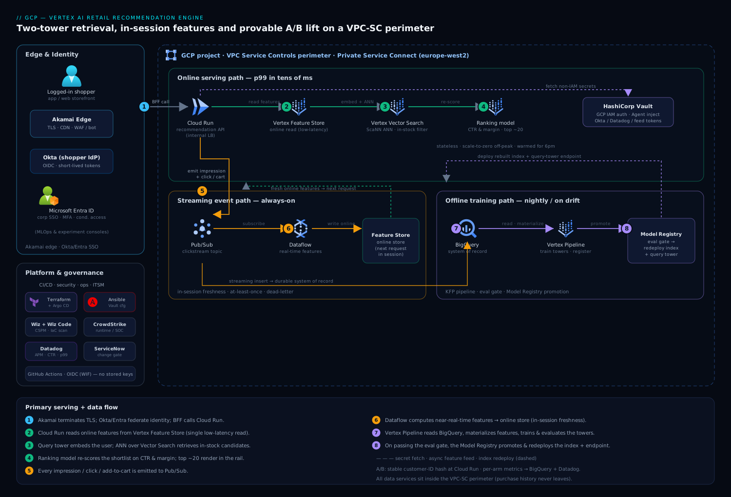
Reading the diagram: a shopper’s request enters through the edge into the Cloud Run serving tier, which reads features, embeds the user, retrieves candidates from Vector Search and ranks them back into the rail; underneath, the Pub/Sub → Dataflow streaming path refreshes features as customers act, while the BigQuery → Vertex AI Pipelines training path rebuilds the towers and the index on a schedule — three paths on three clocks, sharing one set of features.
The platform runs three distinct paths that share infrastructure but live on different schedules, and keeping them separate in your head is the first step to operating this well: an offline training path that learns the towers from history, an online serving path that answers recommendation requests in real time, and a streaming event path that keeps features fresh as customers act.
Serving path, following the request as a shopper sees it:
- A logged-in customer opens the app or storefront. The edge is Akamai — TLS termination, global anycast, CDN for the static catalog imagery, and WAF/bot mitigation so scrapers and credential-stuffers never reach the origin. Customer identity is federated through Okta as the consumer/workforce IdP (brokered to Microsoft Entra ID for the corporate merchandising and data-science staff who administer the platform), so the storefront carries a verified user token and the back-office tools enforce SSO and conditional access.
- The storefront’s backend-for-frontend calls the recommendation service running on Cloud Run. Cloud Run is the deliberate choice for the serving tier: it scales to zero overnight, scales out automatically to absorb the 6pm spike, and bills per request — you are not paying for idle GKE nodes at 3am. The service runs behind an internal HTTPS load balancer; it is stateless, which is what lets it scale horizontally without coordination.
- The service fetches the shopper’s online features from Vertex AI Feature Store with a single low-latency read — their last-N viewed categories, current cart contents, loyalty segment, recency/frequency aggregates. It pulls any secrets it needs that are not GCP-native identities — the Okta introspection secret, the Datadog API key, a partner pricing-feed token — from HashiCorp Vault via the Vault Agent with GCP IAM auth, so nothing sensitive sits in an environment variable or a container image.
- The service runs the query tower to turn those features into a user embedding, then issues an ANN query against the Vertex AI Vector Search index (the deployed item embeddings) to retrieve the few hundred nearest candidate SKUs — filtered server-side for what is in stock at this customer’s store and not on a suppression list (allergens the customer flagged, age-restricted items, already-purchased one-offs).
- A lightweight ranking model re-scores that shortlist with richer features — predicted click-through and predicted margin — so the final order optimizes for revenue, not just relevance. The top ~20 SKUs, hydrated with price and imagery, stream back and render in the rail. Every served impression and the user’s subsequent click or add-to-cart is emitted as an event.
Streaming event path, independent and always-on: every storefront interaction — page view, product view, add-to-cart, purchase — is published to Pub/Sub as a clickstream event. Two subscribers consume the same stream. A Dataflow streaming job computes near-real-time features (this session’s category affinities, rolling counts) and writes them to the online Feature Store so the next request in the same session reflects what just happened — that is the in-session freshness the CDO demanded. The same events land in BigQuery through its streaming insert path as the durable, queryable system of record for all behavioral data.
Offline training path, on a schedule: BigQuery is the analytical heart — years of transactions, the full clickstream, catalog and inventory snapshots. A Vertex AI Pipeline (the orchestrator, Kubeflow-based) reads training data from BigQuery, engineers features and materializes them to the Feature Store so training and serving compute features the same way (defeating training/serving skew, the single most common cause of “it worked offline and tanked in production”), trains the two towers on Vertex AI custom training, evaluates against held-out data, registers the model in the Vertex AI Model Registry, and — on passing the eval gate — rebuilds and redeploys the Vector Search index and the query-tower endpoint. This pipeline runs nightly for embeddings and is re-triggered whenever drift monitoring fires.
Component breakdown
| Component | Service / tool | Role in the platform | Key configuration choices |
|---|---|---|---|
| Edge | Akamai | TLS, anycast, image CDN, WAF, bot mitigation | Origin shield to the internal LB; cache catalog imagery, never the personalized rail |
| Identity / SSO | Okta + Microsoft Entra ID | Shopper auth (Okta) and corporate SSO for data-science/merch staff (Entra) | OIDC; conditional access on Entra for the MLOps console; short-lived tokens |
| Serving tier | Cloud Run | Stateless recommendation API: feature read → embed → ANN → rank | Min instances for warm peak, scale-to-zero off-peak; concurrency tuned to CPU |
| Retrieval | Vertex AI Vector Search | ANN over item embeddings; in-stock + suppression filtering | ScaNN index; restricts/crowding tags for store & category filters |
| Feature store | Vertex AI Feature Store | Low-latency online features + offline materialization | Online serving for reads; offline store backed by BigQuery for training parity |
| Streaming | Pub/Sub + Dataflow | Clickstream ingest; real-time feature computation | At-least-once delivery; dead-letter topic; windowed aggregations |
| Analytics / lake | BigQuery | System of record; training data; experiment analysis | Streaming inserts; partitioned + clustered tables; scheduled queries |
| Training / orchestration | Vertex AI Pipelines + Training | Build, train, evaluate, register the towers | KFP components; eval gate; Model Registry promotion |
| Secrets | HashiCorp Vault | Okta introspection, Datadog key, partner feed tokens | GCP IAM auth; dynamic leases; Vault Agent injection |
| CSPM / data posture | Wiz + Wiz Code | Cloud posture, sensitive-data exposure, IaC scanning | Agentless scan of BigQuery/buckets; Wiz Code gates Terraform in CI |
| Runtime security | CrowdStrike Falcon | Runtime threat detection on build/runner hosts and any GKE nodes | Sensor on CI runners and node pools; detections to the SOC |
| Observability | Datadog | Service APM, infra metrics, and model-performance dashboards | Agent + OTel traces; custom metrics for CTR, latency, model version |
| ITSM / approvals | ServiceNow | Model-promotion change approvals, incident records | Change gate before a model serves prod; auto-ticket on drift breach |
| CI/CD + IaC | GitHub Actions + Argo CD + Terraform | Build/test/deploy; GitOps rollout; infra as code | OIDC to GCP (no stored keys); Argo CD syncs Cloud Run revisions |
| Config mgmt | Ansible | Configure the self-managed Vault cluster and any VM appliances | Idempotent playbooks; pulls no secrets into the repo |
A few of these choices deserve the why, because they are the ones teams get wrong.
Why the Feature Store is non-negotiable, not a nice-to-have. The subtlest bug in any recommender is training/serving skew: the offline pipeline computes “30-day category purchase count” one way and the online service computes it slightly differently, so the model sees inputs in production it never saw in training and quietly degrades. A Feature Store fixes this by being the single place a feature is defined and computed — the training pipeline materializes features into the offline store, and the serving path reads the identical feature definitions from the online store. One definition, two read paths, no skew.
Why Vector Search instead of scoring everything. Restating the core trick because it is load-bearing: at 250,000 SKUs and tens of thousands of QPS, you cannot score the full catalog per request. Vertex AI Vector Search (built on Google’s ScaNN) does approximate nearest-neighbor in single-digit milliseconds and supports filtering via restricts — so “only items in stock at store 1183, excluding suppressed categories” is applied inside the index, not by fetching candidates and filtering in app code. Retrieval is the cheap funnel; ranking is the expensive polish on a shortlist of hundreds.
Why Cloud Run, not GKE, for serving. Recommendation traffic is spiky — a 6pm dinner-hour and pre-holiday peak many times the 3am trough. A stateless, autoscaling, scale-to-zero serverless tier matches that curve and the bill to it. GKE would mean paying for provisioned nodes through the quiet hours, and the serving logic (read features, embed, query ANN, rank) holds no state that needs a long-lived pod. Keep min-instances warm enough to absorb the peak’s leading edge without cold-start latency, and let it scale from there.
Implementation guidance
Provision with Terraform, and make the data boundary the first deliverable. The security team’s veto is about customer purchase history, so the network and IAM posture is the foundation, not an afterthought.
- A VPC with VPC Service Controls drawing a perimeter around BigQuery, Cloud Storage, the Feature Store, and Vector Search — so even a leaked credential cannot exfiltrate purchase data to a project outside the perimeter.
- Private Service Connect / private endpoints for the Vertex AI services and BigQuery, with public access off, so data-plane traffic never traverses the public internet.
- Least-privilege service accounts: the Cloud Run runtime SA gets only
aiplatform.userscoped for online prediction and Feature Store reads; the pipeline SA gets BigQuery read and Vertex AI training; no human holds standing write to the prod model endpoint. - The Pub/Sub topics, Dataflow templates, and BigQuery datasets (partitioned by event date, clustered by customer and SKU).
A minimal Terraform shape for the serving tier communicates the intent — internal ingress, dedicated SA, autoscaling bounds:
resource "google_cloud_run_v2_service" "recs" {
  name     = "reco-serving-prod"
  location = "europe-west2"
  ingress  = "INGRESS_TRAFFIC_INTERNAL_LOAD_BALANCER"  # not public

  template {
    service_account = google_service_account.reco_runtime.email
    scaling {
      min_instance_count = 6     # warm for the 6pm peak's leading edge
      max_instance_count = 400   # headroom for pre-holiday surge
    }
    containers {
      image = "europe-docker.pkg.dev/${var.project}/reco/serving:${var.git_sha}"
      resources { limits = { cpu = "2", memory = "2Gi" } }
    }
  }
}
The pipeline that builds and ships this runs in GitHub Actions, authenticating to GCP via Workload Identity Federation (OIDC) so there is no stored service-account key to leak — a hard lesson the platform team intends never to repeat. Argo CD then drives the GitOps rollout: a new Cloud Run revision is declared in the config repo, Argo CD reconciles it, and a model-serving change is therefore auditable and instantly revertable by reverting a commit. Wiz Code scans the Terraform and container manifests in that pipeline and fails the build on a public-bucket or over-broad-IAM regression before it can ever reach an environment.
Identity: federate the humans, kill the static keys. Shoppers authenticate through Okta; the corporate data scientists and merchandisers who operate the MLOps console and the experiment dashboards authenticate through Microsoft Entra ID with conditional access, so promoting a model to production requires a verified, MFA-backed corporate identity — not a shared key. The residual non-IAM secrets — the Okta introspection secret, the Datadog API key, a partner pricing-feed token — live in HashiCorp Vault, leased dynamically and injected by the Vault Agent, never written into a Cloud Run env var or baked into an image. Ansible configures that self-managed Vault cluster and any virtual appliances (for example, a partner-supplied pricing or fraud appliance that must run as a VM image) idempotently, so the security configuration is code, not a console click someone forgets.
Feature and index wiring. Define every feature once in the Feature Store registry. Materialize from BigQuery for training; serve from the online store at request time. Co-locate the Vector Search index, the Feature Store online store, and Cloud Run in the same region as the BigQuery dataset — a cross-region hop in the serving path is latency you cannot afford in a 40ms budget. Rebuild the index from the freshly trained candidate tower as the final pipeline step, and deploy it behind a new endpoint so a bad index can be rolled back by repointing traffic.
A/B experimentation: proving the lift
This is the section the CFO cares about, and it is where most recommender projects quietly fail — they ship a model that looks smarter and never prove it earns more. The engine is built for experimentation from day one.
Traffic is split at the serving tier by a stable hash of the customer ID into arms — control (the old merchandiser rail or the incumbent model) versus one or more challenger models. The split is deterministic so a given shopper always sees a consistent experience for the experiment’s duration, and it is configured, not coded, so merchandising can launch a test without a deploy. Every served impression is tagged with its experiment arm and model version and flows through Pub/Sub into BigQuery, where the analysis is a scheduled query: per arm, the add-to-cart rate, conversion rate, revenue per session, and average order value, with a statistical-significance test so “the challenger wins” is a defensible claim, not a vibe.
| Stage | Mechanism | What it answers |
|---|---|---|
| Online split | Stable customer-ID hash at Cloud Run | Which shoppers see which model, consistently |
| Metric capture | Impression + outcome events → Pub/Sub → BigQuery | Per-arm CTR, conversion, revenue/session, AOV |
| Live monitoring | Datadog dashboards on the same metrics, by model version | Is a challenger silently tanking right now |
| Decision | BigQuery scheduled query with significance test | Did the lift clear the bar to promote |
The crucial pairing is Datadog for the live view and BigQuery for the verdict. Datadog dashboards — fed custom metrics tagged with model version and experiment arm — show CTR, p99 latency, and error rate per arm in real time, so if a freshly promoted challenger is dropping conversion or blowing the latency budget, an alert fires and the arm can be cut in minutes via config, not after a week of lost revenue. BigQuery is where the statistically sound end-of-experiment decision is made and where merchandising gets the revenue number to take to the CFO. Promotion of a winning model to 100% of traffic passes through a ServiceNow change approval, giving merchandising leadership and the platform owner a documented gate before a model owns the homepage.
Going deeper
This section is for the reader who will actually build or operate the engine. It opens each box: how the towers learn, what ScaNN is really doing, how to read the evaluation numbers, where the milliseconds go, how freshness runs on three clocks, how cold-start is designed for, and how the managed alternative compares.
Inside the two towers: how they learn a shared map
Each tower is a small neural network — typically a few dense layers — that maps raw features to a fixed-length embedding vector (say 64 or 128 numbers). The query tower consumes user/context features; the candidate tower consumes item features. Training shows the model many real (user, engaged-item) pairs and optimizes a dot-product (or cosine) similarity so a user’s vector lands close to the items they truly engaged with and far from everything else. In practice this is built with TensorFlow Recommenders (TFRS) or Vertex AI’s two-tower built-in algorithm, then the trained candidate encoder is used to embed the whole catalog.
The trick that makes training affordable is in-batch negatives: for a training batch of, say, 4,096 (user, positive-item) pairs, every other item in the batch is treated as a negative for a given user. One batch therefore yields thousands of cheap negatives without a separate sampling step, and the loss is a sampled softmax over them. Because popular items appear as negatives disproportionately often, production setups apply a log-Q / popularity correction so the model is not unfairly punished for retrieving genuinely popular products.
Matrix factorization is the linear ancestor of this. Classic collaborative filtering factorizes the user–item interaction matrix into user factors and item factors — which are exactly embeddings whose dot product predicts affinity. You can train one in pure SQL with BigQuery ML:
CREATE OR REPLACE MODEL `proj.reco.mf_candidates`
OPTIONS (
  model_type    = 'matrix_factorization',
  user_col      = 'customer_id',
  item_col      = 'sku',
  rating_col    = 'implicit_rating',   -- e.g. view=1, cart=3, purchase=5
  feedback_type = 'implicit',
  wals_alpha    = 40
) AS
SELECT customer_id, sku, implicit_rating
FROM `proj.reco.interactions`;
It is a superb baseline — cheap, transparent, entirely in BigQuery — and the factors it produces can even be loaded straight into Vector Search. Its limits are exactly what two-tower fixes: matrix factorization is transductive (it only knows users and items seen in training, so it cannot embed a brand-new SKU) and it cannot use rich features (price band, brand, time of day, cart contents). Two-tower generalizes matrix factorization by replacing the lookup-table factors with feature-driven towers — which is precisely why it handles cold-start and context that plain factorization cannot. (One operational caveat: BigQuery ML matrix-factorization training requires a BigQuery reservation with assigned slots — it does not run on pure on-demand billing.)
Inside ScaNN and Vertex AI Vector Search
Retrieval is an approximate nearest-neighbour (ANN) search, and Vertex AI Vector Search is Google’s productization of ScaNN (Scalable Nearest Neighbors). Exact nearest-neighbour over 250,000+ vectors per request is too slow, so ScaNN does three things: it partitions the vector space into a tree of leaves (a query searches only a few nearby leaves, not all of them); it quantizes vectors with anisotropic (score-aware) quantization so approximate dot products stay accurate where it matters; and it rescores the top few with full-precision vectors. This is the “tree-AH” (tree + asymmetric hashing) algorithm.
You do not implement any of that — you tune it. The knobs that matter:
| Knob | Where | Effect |
|---|---|---|
distanceMeasureType |
Index build | DOT_PRODUCT_DISTANCE for dot-product-trained towers; COSINE_DISTANCE (auto unit-normalizes); SQUARED_L2_DISTANCE for Euclidean |
leafNodeEmbeddingCount / approximateNeighborsCount |
Index build | Leaf granularity and how many candidates to gather before rescoring — higher = better recall, more compute |
fractionLeafNodesToSearchOverride |
Query time | Search more leaves for higher recall at higher latency — your main real-time recall/latency dial |
| Restricts (allow/deny tokens) | Index + query | Server-side filtering — e.g. in_stock_store=1183, NOT suppressed_category, applied inside the index |
| Numeric restricts | Index + query | Range filters (price ≤ X, age-rating ≤ Y) evaluated in the index |
| Crowding | Query time | Cap results per attribute (e.g. max 3 per brand) so one brand cannot dominate the rail |
Two update paths keep the index current: a batch update rebuilds the whole index from a fresh embedding export (the nightly job), while a streaming update upserts individual vectors within seconds — how a brand-new SKU becomes retrievable the same day it is listed, without waiting for a full rebuild.
The two “recalls”, and reading offline metrics honestly
“Recall” is overloaded here, and conflating the two is a classic mistake:
- Model recall@k — of the items a user actually engaged with, how many appear in the top-k the model would retrieve (measured against exact/brute-force search). This grades the quality of the learned embeddings.
- ANN recall — of the true top-k nearest vectors, how many the approximate search actually returns (measured against a brute-force index over the same vectors). This grades the search approximation, not the model.
You can have excellent model recall and poor ANN recall (search tuned too aggressively for latency), or vice versa. Keep a small brute-force index alongside the ScaNN index precisely so you can measure ANN recall and set the latency dial at the knee of the curve.
| Stage | Metric | What it tells you |
|---|---|---|
| Retrieval | recall@k, hit-rate@k | Did the funnel’s first stage surface the right candidates at all |
| Retrieval (search) | ANN recall vs brute force | Is the approximation costing you real candidates |
| Ranking | AUC-ROC, log-loss, NDCG@k | Does the ranker order the shortlist well and predict engagement calibratedly |
| Whole system | catalog coverage, diversity/novelty | Are you recommending the long tail or just the same hits |
The essential humility: offline metrics are a proxy, not the verdict. They are computed on logged behavior that was itself shaped by the old model (presentation and feedback bias), so an offline win does not guarantee an online lift. That is why the A/B test — not the offline dashboard — decides what ships. Expect an offline/online gap and treat a disagreement as a diagnosis, not a disappointment.
Where the milliseconds go
A 40 ms p99 serving budget is spent, not given. Decompose it:
- Feature fetch from the online store — single-digit ms if you use the low-latency Optimized online store and colocate it in the serving region.
- Query-tower inference — a few ms for a small MLP on CPU. For returning users whose long-term features rarely change, precompute the user embedding offline and only fold in the fast-changing session signal at request time.
- ANN query against Vector Search — single-digit ms, governed by the recall dial above.
- Ranking — a few ms, because you score only a few hundred candidates, not 250,000.
- Everything else — network hops, serialization, suppression/inventory joins, and hydrating the winners with price and imagery.
The two silent killers are a cross-region hop (put Vector Search, the online store, Cloud Run, and BigQuery in one region) and a cold Cloud Run pool at the peak’s leading edge (keep min-instances warm ahead of the 6pm surge).
Freshness runs on three clocks
Beginners hear “keep it fresh” as one thing; production runs several cadences at once:
| Clock | Cadence | Mechanism | Keeps fresh |
|---|---|---|---|
| Streaming features | seconds | Pub/Sub → Dataflow → online Feature Store | This session’s behavior (just added nappies) |
| New-SKU upsert | minutes | Vector Search streaming update | A newly listed product becomes retrievable same-day |
| Embedding rebuild | nightly | Vertex AI Pipeline exports item embeddings, batch-rebuilds the index | Item vectors reflect the latest interactions |
| Full retrain | weekly-ish or on drift | Retrain both towers, re-evaluate, re-register | The learned model itself, when patterns shift |
Crucially, in-session freshness is a feature-store write problem, not a retrain problem — the model does not change when a shopper adds an item; the feature it reads changes, and the query tower re-embeds on the next request.
Cold-start and the exploration trap
Two-tower handles the item cold-start far better than matrix factorization because the candidate tower ingests content features — a brand-new SKU with a known category, brand, and price band gets a sensible embedding on day one, before it has a single interaction. User cold-start (an anonymous or first-time shopper) has no personal history, so you fall back to popularity-and-context rails (trending in this store, seasonal, category-entry) and personalize as signal arrives within the session.
The subtler trap is the feedback loop: the engine only learns from items it shows, so a purely exploitative recommender starves new items of the impressions they need to prove themselves, and your logs quietly encode the old model’s biases. Counter it with a little exploration — an epsilon-greedy or bandit re-rank, or a diversity/novelty boost that guarantees new and long-tail items a slice of impressions — so the system keeps learning rather than calcifying around yesterday’s winners.
Feature Store internals and point-in-time correctness
The modern Vertex AI Feature Store is built on BigQuery: you register Feature Groups (pointing at BigQuery source tables or views) and Feature Views, and sync them to a Feature Online Store for low-latency reads. Pick the online store type by need — Bigtable-backed for very high throughput and large keyspaces, Optimized for the lowest read latency in a real-time path like this one.
The advanced correctness concern when you build training data is point-in-time correctness. A training row’s label is “did the user engage at time T”; its features must be the feature values as of time T, never today’s values. Fetch “30-day category count as of the event timestamp,” not the current count, or you leak the future into training and the model looks brilliant offline and fails live. The Feature Store’s offline/point-in-time serving (an as-of join in BigQuery) exists precisely to produce leakage-free training sets — the same discipline that, on the serving side, defeats training/serving skew.
The managed alternative in depth: Vertex AI Search for commerce
If you would rather not own towers, indexes, and pipelines, Vertex AI Search for commerce (the evolution of Recommendations AI / the Retail API) packages this whole engine as a service. You import a product catalog and a stream of user events (views, add-to-carts, purchases), and Google trains and serves the models behind an API. You choose a model type by the placement it fills:
| Model type | Placement it fills |
|---|---|
recommended-for-you |
Personalized homepage rail |
others-you-may-like |
Product-detail page |
frequently-bought-together |
Cart / add-on upsell |
similar-items |
“More like this” |
buy-it-again |
Reorder rail for consumables (very apt for grocery) |
page-level-optimization |
Which rail to show where, chosen by the service |
The trade is the usual build-vs-buy one: you gain speed-to-launch, Google-managed retraining, and no ANN tuning; you give up deep control over features, the ranking objective (e.g. optimizing margin rather than clicks), and portability. A pragmatic pattern is to launch on Search for commerce to prove personalization moves money, then graduate to the custom two-tower stack when you need bespoke features, margin-aware ranking, or tighter latency and cost control. For the broader enterprise operating model around either choice — identity, ITSM, security posture, org design — see the companion enterprise architecture for GCP retail recommendations; this lesson stays on the engine.
Enterprise considerations
Security & data posture. The architecture is Zero-Trust by construction: identity-based access only, least-privilege service accounts, and a VPC Service Controls perimeter so customer purchase history physically cannot leave to an unauthorized project. Layer on top: (a) Wiz running continuous CSPM and sensitive-data scanning across BigQuery, Cloud Storage, and the Feature Store, alerting the moment a dataset drifts to broader access or a bucket turns public — the posture backstop behind the IAM policy; (b) Wiz Code shifting that same checking left into the Terraform/container pipeline so misconfigurations are caught pre-merge; © CrowdStrike Falcon sensors on the CI runners and any GKE node pools for runtime threat detection, feeding the retailer’s SOC; (d) a drift or guardrail breach auto-raising a ServiceNow incident so security and MLOps get a ticket, not just a log line. Org Policy denies public ingress on the Vertex AI and serving resources, and Wiz independently verifies the policy is actually holding.
Cost optimization. Compute and data scanning dominate, and both grow with success, so engineer for them from day one.
| Lever | Mechanism | Typical effect |
|---|---|---|
| Serverless serving | Cloud Run scale-to-zero off-peak, autoscale to peak | Pay for the dinner-rush, not 3am idle |
| Retrieval funnel | ANN to a few hundred candidates, rank only the shortlist | Avoids scoring 250k SKUs per request |
| Embedding cadence | Rebuild item embeddings nightly, not per-request | Amortizes training cost across millions of calls |
| BigQuery hygiene | Partition + cluster tables; scheduled rollups; BI Engine for dashboards | Cuts bytes scanned per analytical query |
| Feature reuse | One feature definition serves train + online | No duplicate compute, no skew-debugging cost |
Tag spend by environment and pipe BigQuery and Cloud Run cost metrics to Datadog, which the platform team uses for the showback dashboard the CDO and CFO see.
Scalability. Each tier scales independently. Cloud Run scales on concurrent requests; Vector Search scales by adding replicas to the deployed index for query QPS; the Feature Store online store scales its serving nodes for read throughput; Pub/Sub and Dataflow scale on backlog depth, with the streaming job’s autoscaler matching the clickstream’s diurnal curve. BigQuery’s analytical capacity is elastic by design. The natural ceiling at peak is feature-read and ANN-query latency under load, which is why the index and online store are over-provisioned and warmed ahead of the known dinner-hour and pre-holiday spikes rather than discovered cold.
Failure modes, and what each one looks like. Name them before they page you.
- Cold start at the peak’s leading edge — Cloud Run scaled to zero overnight and the 6pm surge hits a cold pool, so the first wave of shoppers eats container start latency and the rail renders late. Mitigation: min-instances warmed ahead of the known peak; scheduled scale-up before 6pm.
- Stale features / streaming lag — Dataflow falls behind, so in-session signal arrives late and the just-added-to-cart nudge does not appear. Mitigation: monitor subscription backlog as a first-class SLO; autoscale the streaming job; a dead-letter topic so one poison event does not stall the pipeline.
- Cold-start items and users — a brand-new SKU has no engagement history and a first-time shopper has no profile, so pure two-tower retrieval has little to go on. Mitigation: content-based item features (category, brand, attributes) give new SKUs a reasonable embedding immediately; fall back to popularity-and-context rails for anonymous or brand-new users.
- Training/serving skew — a feature computed differently offline vs online silently degrades quality with no error. Mitigation: the shared Feature Store definition, plus Vertex AI model monitoring on feature drift between training and serving distributions.
- A bad model promoted — a challenger wins offline but tanks live conversion. Mitigation: the staged A/B rollout, the Datadog live guardrail that cuts the arm in minutes, and instant rollback by repointing serving traffic to the prior endpoint via Argo CD.
Reliability & DR (RTO/RPO). Decide the numbers per tier. BigQuery is multi-region-durable and is the recoverable source of truth for all behavioral and training data, so the engine is rebuildable from it. The serving tier is stateless and regional — for DR, deploy the Cloud Run service, a replicated Vector Search index, and the online Feature Store in a paired region and fail over at the load-balancer/Akamai layer. A pragmatic target for this platform: RTO 15 minutes, RPO near-zero for the behavioral event stream (Pub/Sub buffers and re-drives), with the model and index rebuildable from BigQuery within hours if lost. Critically, the storefront must degrade gracefully: if the recommendation service is unavailable, the rail falls back to a cached popularity list rather than failing the page — a recommender outage must never take down the homepage.
Observability. Instrument the serving request end to end in Datadog with OpenTelemetry: one trace covering feature-read → embed → ANN → rank, with timing on each hop and the model version as a tag, so a latency regression is attributable to a specific stage and release. Emit the metrics the business actually cares about — recommendation CTR, add-to-cart rate, conversion and revenue per session by model version, plus p99 serving latency and streaming backlog. The model-performance dashboards in Datadog are the daily operational view; BigQuery scheduled queries are the rigorous periodic verdict. Vertex AI model monitoring watches feature and prediction drift and, on breach, re-triggers the training pipeline and opens a ServiceNow ticket. New models pass a ServiceNow change gate before serving production, giving the business a documented promotion record.
Governance. Pin and register every model version in the Vertex AI Model Registry with its training-data snapshot and eval metrics, so a production model is always traceable to exactly what produced it and promotion is an auditable event, never a floating “latest.” Keep feature definitions, pipeline code, and the experiment configuration in version control, reviewable and revertable. Apply Org Policy to deny public ingress and require the VPC-SC perimeter, with Wiz as the independent check that the controls are real. Retain the clickstream under the retailer’s data-retention and consent regime, honoring deletion requests across BigQuery and the Feature Store, since purchase history and behavioral data are personal data.
Explicit tradeoffs
Accept these or do not build it. A two-tower retrieval engine adds real moving parts — a streaming pipeline, a feature store to keep consistent, embedding rebuilds, and retrieval quality you must measure and tune. Latency is the sum of feature read and embedding and ANN and ranking; budget all four. Approximate nearest-neighbor is approximate — you trade a sliver of recall for the latency that makes real-time serving possible, and ranking on the shortlist is what recovers quality. Cold start is a genuine weakness of any embedding recommender and needs the content-feature and popularity-fallback mitigations baked in, not bolted on. The VPC-SC perimeter and private endpoints that make the security team sign cost you setup complexity and remove public debugging shortcuts. And the A/B harness, the dual Okta/Entra identity planes, and the Vault-held secrets are overhead you could skip for a single-store pilot and absolutely cannot skip for a 1,400-store, regulated-data rollout.
The alternatives, and when they win. If your catalog is small and traffic modest, a nightly co-occurrence/matrix-factorization batch served from a cache is far simpler and may be enough — graduate to two-tower when real-time freshness and a large catalog demand it. If you want a managed black box and less ML ownership, Vertex AI Search for commerce / Recommendations AI packages much of this as a service — you trade control and customizability for speed-to-launch. If your problem is really ranking a known small set rather than retrieving from a huge catalog, you may not need the retrieval tower at all — a single ranking model suffices. And if personalization is not yet a proven revenue lever for your business, start with the experimentation harness and a simple popularity model, prove the rail moves money, and only then invest in the full Vertex AI stack described here.
The shape of the win
For the retailer, the payoff is not “an AI rail.” It is that a shopper who just put nappies in their cart sees formula and wipes in the recommendation slot before checkout, the rail rendered inside the page’s latency budget, the purchase history never left the GCP perimeter — and, the sentence that funds the platform, merchandising can show the CFO a BigQuery-backed, statistically significant lift in revenue per session from the controlled rollout before the model ever owned 100% of the homepage. Everything upstream — the two towers, the Feature Store parity, the Pub/Sub clickstream, the Vector Search funnel, the Okta-to-Entra identity planes, the Vault-held secrets, the Wiz posture scanning, the Datadog model dashboards — exists to make a head of merchandising, a CISO, and a CFO each say yes. The architecture here is the destination; start with the experiment and a simple model if you must, but this is where real-time, at-scale, provable retail personalization on GCP has to land.
Practice challenges
Work these in order; each has a worked solution. They escalate from arithmetic you can do on paper to production tuning decisions.
1. (Beginner) The funnel math. The catalog holds 250,000 SKUs. Retrieval returns 300 candidates; ranking trims to 20. What fraction of the catalog does the ranking model score per request, and why does the two-stage design matter?
<details><summary>Solution</summary>
Ranking scores 300 / 250,000 = 0.12% of the catalog. The point: ranking is the expensive, feature-rich pass, so you only ever run it on a few hundred candidates that the cheap ANN retrieval already narrowed down. Scoring all 250,000 with the ranker every request would blow both the latency budget and the bill. Why: the funnel exists to make per-request cost roughly independent of catalog size. </details>
2. (Beginner) Choose the distance measure. You trained two-tower embeddings with a dot-product objective and did not normalize the vectors. Which distanceMeasureType should the Vector Search index use, and what would change if you picked COSINE_DISTANCE?
<details><summary>Solution</summary>
Use DOT_PRODUCT_DISTANCE to match the training objective. COSINE_DISTANCE unit-normalizes vectors, discarding magnitude — which for dot-product-trained embeddings changes the ranking (magnitude often encodes popularity/confidence). Mismatching the serving distance to the training objective is a quiet quality bug. Why: the index must score vectors the same way the model was trained to.
</details>
3. (Intermediate) A one-SQL baseline. Before committing to two towers, you want a candidate generator you can ship this week. Write the BigQuery ML that produces user/item factors from an interactions(customer_id, sku, implicit_rating) table, and name one limitation.
<details><summary>Solution</summary>
CREATE OR REPLACE MODEL `proj.reco.mf_baseline`
OPTIONS (model_type='matrix_factorization', user_col='customer_id',
         item_col='sku', rating_col='implicit_rating',
         feedback_type='implicit', wals_alpha=40) AS
SELECT customer_id, sku, implicit_rating FROM `proj.reco.interactions`;
Limitation: it is transductive — it cannot score a brand-new customer or SKU unseen in training (no cold-start), and it uses no side features. Also, MF training needs a BigQuery reservation. Why: it’s a fast, transparent baseline to beat, and its weaknesses motivate the two-tower upgrade. </details>
4. (Intermediate) Trace in-session freshness. A shopper adds nappies to the cart. List the components, in order, that must act for the next request to recommend formula and wipes, and name the one that makes it fast enough to feel “in-session.”
<details><summary>Solution</summary>
add-to-cart event → Pub/Sub → Dataflow (updates the session's category-affinity feature) → online Feature Store → next request's feature fetch → query tower re-embeds the user → Vector Search returns formula/wipes → ranking. The online Feature Store (Optimized) low-latency write-then-read is what makes it in-session, and the model never retrains. Why: freshness here is a feature-update latency problem, not a model-training one.
</details>
5. (Advanced) The offline win that didn’t pay. You lifted offline recall@50 by 4%, but the A/B test shows no revenue lift. Give three plausible causes and how you’d distinguish them.
<details><summary>Solution</summary>
(a) Offline/online gap / feedback bias — recall was measured on logs shaped by the old model, so the “win” is partly illusory; check by slicing metrics by segment and comparing to online per-arm outcomes. (b) Right candidates, wrong order/objective — retrieval improved but ranking (or a clicks-not-margin objective) didn’t surface them; check ranking-stage NDCG and the business metric per arm. © Production regression — ANN recall or p99 latency degraded under load, eating the gain; check the brute-force-vs-ScaNN recall and the latency/error dashboards per arm. Why: offline metrics are a proxy; disagreement with the A/B test is a diagnostic signal, not noise. </details>
6. (Advanced) Set the recall/latency operating point. Your retrieval p99 budget is 8 ms. Which build-time and query-time knobs trade ANN recall for latency, and what procedure finds the right setting?
<details><summary>Solution</summary>
Build-time: leafNodeEmbeddingCount / approximateNeighborsCount and shard size. Query-time: fractionLeafNodesToSearchOverride — searching more leaves raises recall and latency. Procedure: stand up a brute-force index as ground truth, then sweep the fraction upward, measuring ANN recall@k and p99 at each step; stop at the knee where recall plateaus while still inside 8 ms. Why: ANN recall is a tunable dial, so you deliberately pick the point on the recall-vs-latency curve that fits the budget.
</details>
Common beginner mistakes
- “The model scores the whole catalog for each shopper.” It does not, and it could not at 250,000 SKUs and peak QPS. Retrieval (ANN) narrows the catalog to a few hundred; only that shortlist is ranked. Right model: a two-stage funnel — cheap wide retrieval, then expensive narrow ranking.
- “Vector Search returns the exact nearest items.” It returns approximate neighbours — that approximation is the whole reason it is fast. Treat ANN recall as a number you measure (against a brute-force index) and tune, not a guarantee. Right model: you trade a sliver of recall for a huge latency win, and you own where on that curve you sit.
- “Better offline metrics mean more revenue.” Offline recall/NDCG are computed on logs biased by the old model; they are a proxy. The A/B test is the arbiter. Right model: ship on lift; use offline metrics to decide what is even worth testing.
- “Freshness means retraining the model.” In-session freshness is a feature-store update, not a retrain — the shopper’s just-added item changes a feature the query tower reads, not the tower’s weights. Retraining runs on a much slower clock. Right model: three cadences — streaming features (seconds), embedding rebuild (nightly), full retrain (weekly/on drift).
- “Retrieval and ranking are the same model doing one job.” They optimize different things: retrieval maximizes recall over a huge space with light features; ranking maximizes a business objective (CTR, margin) over a tiny shortlist with rich features. Right model: two models, two objectives, in sequence.
- “The model will handle cold-start on its own.” A pure ID-embedding model cannot represent an item or user it never saw. New items need content features; new users need popularity/context fallbacks; and without a little exploration, new items never earn the impressions to prove themselves. Right model: cold-start is a design requirement you build for, not an emergent property.
- “Features computed offline and online will naturally match.” They won’t unless you force them to. Two code paths computing “30-day category count” will drift, and the model degrades silently. Right model: define each feature once in the Feature Store; training materializes it, serving reads the identical definition — plus point-in-time joins so training never sees the future.
Glossary
- Recommendation engine — software that predicts which items to show a specific user, here to fill a “Recommended for you” rail.
- Candidate generation / retrieval — the first funnel stage: cheaply narrow the full catalog to a few hundred plausible items.
- Ranking — the second stage: score and order that shortlist with richer features to optimize a business objective (clicks, conversion, margin).
- Two-tower model — two neural networks (query tower for users/context, candidate tower for items) that map into one shared embedding space so similarity is a dot product.
- Embedding — a fixed-length vector of numbers representing a user or item; nearby vectors mean “similar / relevant.”
- Query tower / candidate tower — the user-side and item-side encoders of a two-tower model.
- In-batch negatives — a training trick where other items in the same batch serve as negative examples, making training cheap.
- Matrix factorization — classic collaborative filtering that factorizes the user–item matrix into user/item factors (embeddings); a simple baseline, available in BigQuery ML, but transductive and feature-blind.
- ANN (approximate nearest neighbour) — finding near-closest vectors quickly instead of the exact closest slowly; the basis of real-time retrieval.
- ScaNN — Google’s ANN library (tree partitioning + anisotropic quantization + rescoring) that powers Vertex AI Vector Search.
- Vertex AI Vector Search — the managed ANN service that indexes item embeddings and retrieves nearest candidates; formerly Matching Engine.
- Restricts / numeric restricts — allow/deny and range filters applied inside the Vector Search index (e.g. in-stock at this store, price ≤ X).
- Crowding — a query-time cap on results sharing an attribute (e.g. max 3 per brand) to keep the rail diverse.
- Distance measure — how vector similarity is scored: dot-product, cosine, or squared-L2; must match the training objective.
- recall@k — the fraction of the items a user engaged with that appear in the top-k retrieved; the key retrieval-quality metric.
- ANN recall — how well approximate search matches exact search; distinct from model recall@k, and measured against a brute-force index.
- NDCG — Normalized Discounted Cumulative Gain; a ranking metric that rewards relevant items placed high in the order.
- Offline/online gap — the common divergence between offline metric wins and real online lift, because logs are biased by the deployed model.
- Feature Store — the single place features are defined; materialized to an offline store (BigQuery) for training and an online store for low-latency serving.
- Feature View / Feature Group — Vertex AI Feature Store objects that map BigQuery sources into synced, servable features.
- Online store (Bigtable / Optimized) — the low-latency serving backend of the Feature Store; Optimized for lowest latency, Bigtable for very high throughput.
- Materialization — computing feature values and writing them to the store (offline for training data, online for serving).
- Point-in-time correctness — building training rows with feature values as of each event’s timestamp, so the model never sees future data (no label leakage).
- Training/serving skew — the bug where a feature is computed differently in training vs serving, silently degrading quality.
- Cold-start — the problem of recommending for brand-new items (no interaction history) or brand-new users (no profile).
- Clickstream — the stream of user interaction events (page views, product views, add-to-carts, purchases).
- Pub/Sub — GCP’s managed message bus; here it carries the clickstream events.
- Dataflow — GCP’s managed Apache Beam service; here it computes streaming features and writes them to the online store.
- Vertex AI Pipelines — Kubeflow-based orchestration for the train → evaluate → register → deploy workflow.
- Model Registry — Vertex AI’s versioned catalog of trained models, tying a serving model to its training snapshot and metrics.
- A/B test (arm, stable hash) — splitting traffic deterministically (by a hash of customer ID) into control vs challenger arms to measure incremental lift.
- Vertex AI Search for commerce — Google’s managed recommendation/search product (formerly Recommendations AI) — the build-vs-buy alternative to this custom stack.
- p99 latency — the 99th-percentile response time; the budget the rail must render within.
- VPC Service Controls — a security perimeter around GCP data services so data cannot be exfiltrated to projects outside it.