Every pandas lesson so far started from a DataFrame that already existed — a CSV on disk, a table in a database, a JSON payload. Data engineering is the discipline that puts it there: moving and shaping data reliably, at scale, so that the analyst opening a notebook, the dashboard refreshing at 6am, and the ML model retraining nightly all get correct, fresh, query-cheap data without knowing or caring how it arrived. It is the plumbing. When it works, nobody notices; when it breaks, every number downstream is quietly wrong.
The gap between a data script and a data pipeline is the whole subject. A script runs once, on your laptop, and produces the right answer today. A pipeline runs unattended every day for two years, survives the source system going down mid-run, gets re-run three times by a nervous on-call engineer, back-fills six months of history when someone finds a bug, and must produce the same correct answer every single time — no duplicated rows, no doubled revenue, no silently dropped records. This lesson is about the handful of properties — idempotency, incrementality, partitioning, validation, orchestration — that turn the former into the latter, and it demonstrates every one of them on executed output rather than assertion.
Everything in the batch half of this lesson is executed on Python 3.12.3 with pandas 3.0.3 and pyarrow 25.0.0, and the numbers, row counts and file listings are real. The Airflow DAG is parse-validated on apache-airflow 2.10.5 (loaded in a real
DagBagwith zero import errors) but its task bodies were not run against a live scheduler or warehouse. The Kafka producer/consumer code is API-accurate for kafka-python 3.0.8 (every parameter verified by introspection) but was not run against a broker — there is no Kafka cluster here, and I will say so again at the point it matters. Nothing in the streaming section is fabricated runtime output.
Why this matters
You have learned to wrangle a DataFrame: group, merge and clean it, read it from and write it to disk, pull it out of a SQL database. Data engineering is what makes those inputs exist and stay trustworthy. It is the difference between a one-off analysis and a system: the code that runs at 3am when you are asleep, that a colleague re-runs without understanding it, that must not corrupt six months of history because a source file arrived twice.
The single most expensive lesson in the field is that a broken pipeline almost never raises an exception — it hands you a wrong number. A re-run that appends instead of overwrites doubles your revenue. A join to a dimension table with a duplicate key triples a customer’s orders. A CSV read where a Parquet was needed turns a two-second query into a two-minute one and a rupee into a hundred. A missing timezone in a partition key files an event under the wrong day. None of these throw. The analyst notices when the board deck disagrees with Finance, three weeks later, and now you are doing archaeology. Every property this lesson teaches exists to convert one of those silent, downstream, wrong-number failures into a loud, immediate, right-at-the-source one.
The mental model to hold for the whole lesson is a pipeline as a sequence of idempotent, observable steps over partitioned data. Idempotent so a re-run is safe. Observable so you know the row count, the freshness, and where a number came from. Partitioned so a query touches a slice, not the whole history. Get those three right and almost everything else is detail. Get any one wrong and you have a script that happens to be scheduled — which is the most dangerous thing in a data platform, because it looks like a pipeline right up until the day it silently isn’t.
There are two shapes of pipeline, and you need both. Batch processes bounded chunks of data on a cadence — “every night, roll up yesterday’s orders.” Streaming processes an unbounded flow of events as they arrive — “flag a fraudulent transaction within 200 milliseconds.” Most of the world’s data work is batch, it is where you should start, and it is where this lesson spends most of its words; streaming is the specialised tool for genuinely low-latency problems, and the last third of the lesson is an honest map of when you need it and what it costs.
Here is the whole lesson as one picture — two lanes, both ending in the same warehouse:
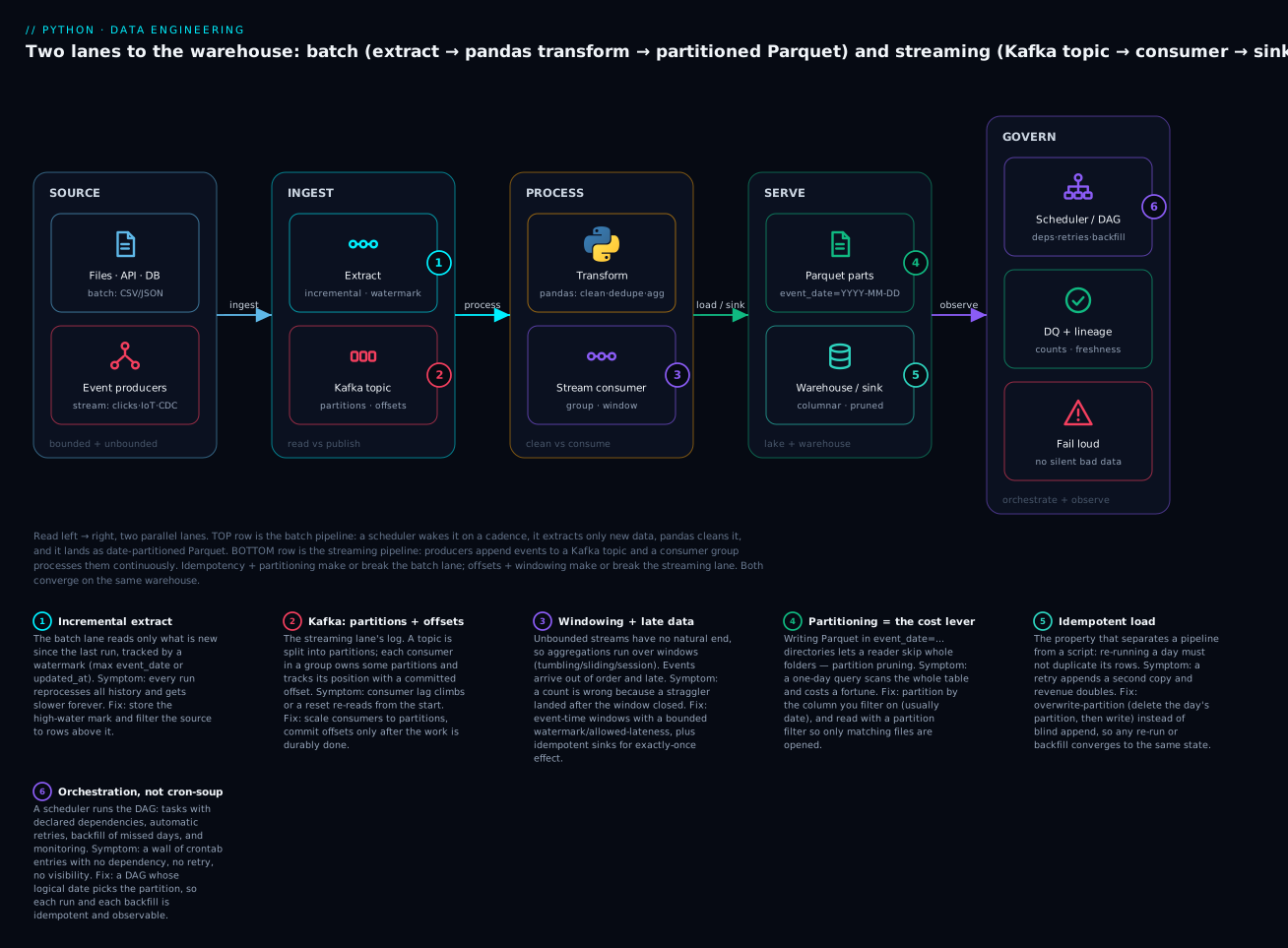
Read it as two lanes. The top lane is batch — extract only new data, clean it with pandas, land it as partitioned Parquet — where idempotency and partitioning are the make-or-break (badges 4, 5) and a scheduler/DAG orchestrates the whole thing (badge 6). The bottom lane is streaming — producers append to a Kafka topic, a consumer group processes continuously — where offsets and windowing are the make-or-break (badges 2, 3). Both lanes converge on the same warehouse, and both are governed by the same data-quality discipline. Every one of those badges is a section of this lesson.
What data engineering is, and ETL vs ELT
Strip away the tooling and data engineering is three verbs repeated forever: Extract data from where it lives, Transform it into a clean, conformed shape, and Load it to where it can be queried. That acronym — ETL — is the oldest three letters in the field, and for decades it described the literal order: pull data out of source systems, run it through a transformation engine that cleaned and joined and aggregated it, then load the finished, analysis-ready tables into a warehouse. The transform happened before the load, on a separate box, because warehouse compute was scarce and expensive and you did not want to waste it on raw, dirty data.
Then cloud warehouses changed the economics and the order flipped. ELT — Extract, Load, Transform — loads the raw data into the warehouse first, cheaply, and does the transformation there, in SQL, using the warehouse’s own elastic compute. Snowflake, BigQuery, Databricks and Redshift made in-warehouse compute so cheap and so scalable that the old reason to transform-before-load evaporated. Loading raw and transforming in place turned out to have real advantages: you keep the raw data (so you can re-transform when requirements change without re-extracting), the transformation is version-controlled SQL that analysts can read and modify, and you are not maintaining a separate transformation cluster. The tool that won the “T” in ELT is dbt, which is essentially “SQL SELECT statements plus dependency management plus tests plus documentation,” and it is now the default way transformations are expressed in a modern warehouse.
| Dimension | ETL (transform then load) | ELT (load then transform) |
|---|---|---|
| Order | Extract → Transform → Load | Extract → Load → Transform |
| Where the T runs | a separate engine (Spark, an ETL server, pandas) | inside the warehouse, in SQL |
| Raw data kept? | often no — only the cleaned output lands | yes — raw lands first, transform reads it |
| Re-transform on new requirements | must re-extract from source | just re-run SQL on the raw you already have |
| Best when | source is heavy/remote; warehouse compute scarce; complex non-SQL logic | cloud warehouse; SQL-expressible logic; analyst-owned transforms |
| Typical stack | pandas / Spark / Informatica → warehouse | Fivetran/Airbyte load → dbt transforms in Snowflake/BigQuery |
| Where Python fits | the whole T (this lesson’s batch ETL) | the E and L (ingestion), orchestration, and non-SQL transforms |
The honest summary: ELT won for the cloud-warehouse world, but ETL never died — it is alive and well wherever the transformation is not naturally SQL (parsing logs, calling an ML model, reshaping nested API payloads, joining across systems the warehouse cannot see), and that is exactly where Python lives. When your transform is a pandas pipeline of clean-dedupe-derive-aggregate, you are doing ETL, and you are doing it in Python because SQL would be miserable for it. The two are not a religious war; a real platform uses both — ELT for the warehouse-native rollups, Python ETL for the awkward ingestion and the non-SQL logic, and one orchestrator scheduling all of it.
Where does the transformed data land? Two related destinations. A data warehouse is a structured, query-optimised store of modelled tables (Snowflake, BigQuery, Redshift) — schema-on-write, SQL-first, built for analytics. A data lake is cheap object storage (S3, GCS, ADLS) holding files — often Parquet — in a schema-on-read layout; you point a query engine at the files. The lakehouse (Delta Lake, Apache Iceberg, Apache Hudi) is the modern convergence: warehouse-like tables (ACID transactions, schema evolution, time travel) built on top of Parquet files in a lake, giving you the cheap storage of a lake with the correctness guarantees of a warehouse. The batch pipeline you build in this lesson writes partitioned Parquet — the raw material of a lakehouse — and the idempotency you will engineer by hand is exactly what Delta and Iceberg give you for free.
| Destination | Stores | Schema | ACID / transactions | Cost | Examples |
|---|---|---|---|---|---|
| Data warehouse | modelled tables | schema-on-write (defined up front) | yes | higher (managed compute + storage) | Snowflake, BigQuery, Redshift |
| Data lake | raw files (Parquet, JSON) | schema-on-read (applied at query) | no (files, not tables) | lowest (object storage) | S3, GCS, ADLS + Athena/Spark |
| Lakehouse | Parquet files as tables | schema-on-read + evolution tracked | yes — on top of files | low storage + table guarantees | Delta Lake, Iceberg, Hudi |
The batch pipeline, built for real
A batch pipeline is the three verbs made concrete. Let us build each one properly, because each has a decision that separates a toy from a system.
Extract: full vs incremental, and the watermark
Extraction pulls data from a source — files on disk or object storage, an HTTP API, a production database, a message queue’s archive. The critical decision is how much you pull each run. A full load re-reads the entire source every time: simple, always correct, and ruinous once the source is large — re-reading a billion-row table nightly to capture yesterday’s ten thousand new rows is pure waste, and it gets slower every day forever. An incremental load pulls only what changed since last time, which is what every real pipeline does past a certain size.
Incremental extraction needs a watermark: a stored high-water mark that says “I have already processed everything up to here.” The next run reads only rows above the watermark, processes them, and advances it. The watermark is usually a monotonically increasing column — an updated_at timestamp, an auto-incrementing ID, or a partition date. The subtle failures live here: a watermark on created_at misses rows that were updated after creation; a watermark compared with > instead of >= (or vice-versa) either skips or double-reads the boundary row; a source clock skewed from yours drops rows near the edge.
| Extract strategy | How it selects rows | Cost per run | Risk |
|---|---|---|---|
| Full load | read everything, every run | grows with total data forever | slow and wasteful at scale; but always complete |
| Incremental (append-only) | WHERE created_at > watermark |
grows with new data only | misses updates to old rows; boundary > vs >= bugs |
| Incremental (upsert) | WHERE updated_at > watermark |
grows with changed data | needs a reliable updated_at; late updates before watermark are missed |
| CDC (change data capture) | read the DB’s transaction log | near-real-time deltas | most complex; needs log access + a CDC tool (Debezium) |
| Snapshot + diff | full extract, diff against last | full read but small load | expensive extract; used when source has no watermark column |
The watermark column you pick decides which changes you can even see:
| Watermark column | Catches | Misses | Boundary risk |
|---|---|---|---|
created_at |
new inserts | updates to existing rows | > skips / >= re-reads the edge row |
updated_at |
inserts and updates | hard deletes; rows updated with no updated_at bump |
needs the source to touch it on every write |
auto-increment id |
new inserts | updates and deletes | gaps from rolled-back transactions |
| partition date | a whole day’s data | intra-day late arrivals | timezone skew at the day boundary |
| CDC log offset | inserts, updates, and deletes | nothing (it is the source of truth) | needs log access + a CDC tool |
Change Data Capture (CDC) is the incremental method taken to its limit: instead of polling a column, you read the database’s own write-ahead log (the same log the DB uses for replication) and capture every insert/update/delete as it commits. Tools like Debezium stream those changes into Kafka, which is the bridge into the streaming half of this lesson — CDC is how a batch warehouse gets fed by a streaming source.
Transform: clean, dedupe, derive, validate — with pandas
The transform is where the pandas lessons pay off. It is the same verbs you already know — clean and normalise, drop duplicates, join, aggregate, handle missing values — now applied as a repeatable, validated stage rather than an ad-hoc notebook. A production transform does five things in order:
| Transform step | pandas tool | Why it is here |
|---|---|---|
| Clean | .str.strip(), .str.title(), pd.to_datetime, .astype() |
normalise whitespace, case, types so keys and categories actually match |
| Dedupe | .drop_duplicates(subset=[key]) |
a retried API call or replayed file delivers the same record twice |
| Derive | .assign(...), arithmetic, .dt accessors |
compute revenue, extract the partition date, bucket values |
| Aggregate | .groupby().agg(), .pivot_table() |
roll events up to the grain the warehouse needs |
| Validate | assertions on schema/nulls/ranges | fail the run loudly rather than load bad data silently |
The validation step is the one beginners skip and seniors never do. A transform that cleans perfectly today will meet a malformed row tomorrow — a null where a price should be, a category no one has seen, a negative quantity, a duplicate that survived the dedupe. The choice is between catching it at the transform (a loud failure, a paged engineer, no bad data downstream) and letting it flow (a silent wrong number, discovered weeks later). A data-quality gate — a block of assertions that raises if any invariant is violated — is cheap insurance:
problems = []
if df["event_id"].duplicated().any():
    problems.append("duplicate event_id after dedupe")
if not set(df["category"]).issubset(VALID_CATEGORIES):
    problems.append(f"unknown category {set(df['category']) - VALID_CATEGORIES}")
if (df["qty"] <= 0).any():
    problems.append("non-positive qty")
if problems:
    raise ValueError("data-quality check failed: " + "; ".join(problems))
Feed that gate a batch with a typo’d category and it stops the pipeline dead, exactly as you want:
ValueError: data-quality check failed: unknown category {'Dairyy'}
That is a real, executed traceback line. The checks worth writing fall into a small set of categories:
| Check type | Asserts | pandas expression | Catches |
|---|---|---|---|
| Schema | expected columns + dtypes present | set(cols) <= set(df.columns) |
a renamed/dropped source field |
| Not-null | required columns have no holes | df[req].isna().any() |
missing prices, unmatched keys |
| Uniqueness | a key is unique | df["id"].duplicated().any() |
a failed dedupe, a fan-out join |
| Range | numbers are in bounds | (df["qty"] <= 0).any() |
negative qty, absurd prices |
| Set membership | categoricals are known values | set(df["cat"]) <= VALID |
typos, new unhandled categories |
| Referential | foreign keys exist in the dim | ~df["cust_id"].isin(dim) |
orphan facts |
| Freshness | newest data is recent enough | df["ts"].max() >= cutoff |
a stalled upstream source |
| Volume | row count is in a sane band | not lo <= len(df) <= hi |
a truncated or duplicated extract |
For richer validation than hand-rolled asserts, Great Expectations (and the lighter Pandera) let you declare a suite of expectations — “column revenue is non-null, between 0 and 100000, and 99% of the time under 5000” — and get a validation report, data docs, and a pass/fail you can wire into the pipeline. The principle is identical; the library just makes the invariants declarative, documented, and testable. Treat data quality as a first-class stage, not a comment.
Load: overwrite, append, or upsert
The load writes the transformed data to its destination, and the mode you choose is the whole idempotency story (which the next section demonstrates in full). Append adds rows — correct for immutable event logs, catastrophic on a re-run because it duplicates. Overwrite replaces everything — safe but wasteful, and it destroys history. Overwrite-partition replaces only the slice this run produced — the sweet spot for date-partitioned data, and the pattern this lesson builds. Upsert/merge (SQL MERGE, Delta merge) updates existing keys and inserts new ones — the correct mode when rows can change, and what CDC pipelines use.
| Load mode | Effect | Idempotent on re-run? | Use when |
|---|---|---|---|
| Append | add rows to the target | No — duplicates every re-run | immutable log where you guarantee one write per record |
| Full overwrite | replace the entire target | Yes | small tables; a full-refresh dimension |
| Overwrite-partition | replace only this run’s partition(s) | Yes | date-partitioned facts (this lesson) |
| Upsert / merge | update matched keys, insert new | Yes | rows mutate; CDC; slowly-changing dimensions |
Real pipelines rarely load in one hop from raw to analytics-ready; they land data in layers, a pattern the lakehouse world calls medallion (bronze → silver → gold) and the dbt world calls staging → intermediate → marts. Bronze/raw is the source data landed as-is, immutable, so you can always re-derive everything downstream from it. Silver/cleaned is the conformed, deduplicated, validated version — the output of your transform, the partitioned Parquet this lesson builds. Gold/marts are the business-level aggregates analysts actually query — revenue by region by day, the tables a dashboard hits. Each layer is a separate, idempotent load, and the value of the split is blast radius: a bug in an aggregate is fixed by re-running gold from silver, without re-extracting from the source, and a new requirement becomes a new gold table over the silver you already trust. The event warehouse you build below is a silver table; the daily rollup in the final step is a gold one.
| Layer | Also called | Holds | Rebuilt from |
|---|---|---|---|
| Bronze | raw / landing / staging | source data, as-is, immutable | the source (re-extract) |
| Silver | cleaned / conformed / core | validated, deduped, typed, partitioned | bronze |
| Gold | marts / serving / aggregates | business rollups analysts query | silver |
File formats and partitioning: the biggest cost lever
Before the pipeline can be idempotent, it has to write files, and which format and how partitioned is the single largest lever on query cost and speed in the entire field. This is not a detail; it is often a 10-to-100× difference in money and minutes, and it is executed here on 500,000 real rows.
Row formats vs columnar: CSV/JSON vs Parquet
CSV and JSON are row formats: values are stored one record at a time, as text. They are human-readable, universal, and the right choice for interchange and small data — and wrong for analytics at scale, for two reasons. First, text is bulky and uncompressed: every number is re-parsed from its decimal string on every read. Second, they are row-oriented, so a query that wants one column out of twenty must still read all twenty off disk.
Parquet is a columnar binary format: values are stored one column at a time, typed, compressed, with statistics (min/max/null-count) per chunk. That layout is transformational for analytics. A query for SUM(revenue) reads only the revenue column and skips the rest (column projection). The per-chunk min/max lets the reader skip chunks that cannot match a filter (predicate pushdown). And typed columns of similar values compress far better than text. Measured on the same 500,000-row, 7-column event frame:
| Format | Size on disk | vs CSV | Notes |
|---|---|---|---|
| JSON lines (text) | 65.0 MB | 0.4× (bigger!) | most verbose — repeats every key on every row |
| CSV (text, no compression) | 24.0 MB | 1.0× (baseline) | universal, human-readable, bulky |
| Parquet, uncompressed | 13.6 MB | 1.8× smaller | columnar layout alone beats text |
| CSV + gzip | 7.5 MB | 3.2× | compresses well but still row-oriented, opaque |
| Parquet + snappy (default) | 8.2 MB | 2.9× | fast codec — the sensible default |
| Parquet + gzip | 6.1 MB | 3.9× | smaller, slower to write |
| Parquet + zstd | 5.3 MB | 4.5× | best ratio; modern default on many platforms |
Parquet with zstd is 4.5× smaller than raw CSV and 12× smaller than JSON lines — and the size is the smaller half of the win. The read speed is the bigger half:
read all cols from CSV        :    228.1 ms
read all cols from Parquet    :     10.7 ms   (21.4x faster than CSV)
read 1 col  from Parquet      :      4.2 ms   (columnar projection: skip 6 of 7 cols)
Reading the whole frame from Parquet is 21× faster than from CSV — no text parsing, no type inference, just typed bytes into typed arrays. Reading a single column is faster still, because columnar storage lets the reader physically skip the other six columns’ bytes. (These millisecond figures are machine- and cache-dependent; the magnitudes — one to two orders of magnitude — are the durable fact.) Compression codecs trade write-time CPU for size:
| Codec | Ratio (this data) | Write speed | Splittable | Use when |
|---|---|---|---|---|
snappy |
2.9× | fast | yes | the safe default — balanced speed and size |
zstd |
4.5× | fast-ish (tunable level) | yes | best all-round; the modern default on many platforms |
gzip |
3.9× | slow | yes | cold/archival data where read is rare |
lz4 |
~2.9× | fastest | yes | write-heavy hot paths |
| none | 1.8× | fastest | yes | rarely worth it — you give up size for little gain |
snappy is the safe default; zstd gives the best ratio at modest cost and is what most modern platforms now standardise on; gzip is smaller but slow; uncompressed is rarely worth it.
Partitioning: the query-cost lever
Columnar format makes each file cheap to read. Partitioning makes it so you read fewer files at all. To partition a dataset is to split it into subdirectories by the value of a column — almost always a date — so that warehouse/events/ becomes:
warehouse/events/
├── event_date=2026-03-01/part-0.parquet
├── event_date=2026-03-02/part-0.parquet
├── event_date=2026-03-03/part-0.parquet
└── event_date=2026-03-04/part-0.parquet
That directory layout (column=value, called Hive partitioning) is not cosmetic — it is a physical index the query engine reads from the path. A query filtered to one day opens one directory and ignores the rest. That is partition pruning, and it is the biggest single cost lever in analytics because cloud warehouses and lake engines bill by bytes scanned. Partition by the column you filter on and a one-day query scans one day’s bytes; forget to, and it scans all of history for every query. Measured on a 10-day, 500,000-row partitioned dataset:
read ALL 10 partitions        :     20.2 ms   (500,000 rows)
read 1 partition (pruned)     :      3.4 ms   ( 49,967 rows, ~1/10th the data)
The pruned read touches roughly a tenth of the data and returns in roughly a tenth of the time — and on a real warehouse where “all partitions” is years of terabytes, that ratio is the difference between a ₹0.05 query and a ₹50 one.
| Partition choice | Effect | When |
|---|---|---|
By date (event_date=…) |
one directory per day; prune to a date range | almost always — most queries filter by time |
| By date + low-card key (region, tenant) | prune on two dimensions | large multi-tenant/multi-region data |
| Too fine (by hour, by user_id) | millions of tiny files — the “small-files problem” | never partition by a high-cardinality column |
| Too coarse (by year) | prune helps little; each partition huge | only for genuinely small or rarely-filtered data |
| Unpartitioned | every query is a full scan | tiny tables, or a staging area before partitioning |
The two ways to get partitioning wrong are opposite and both painful. Partition on a high-cardinality column (a user ID, a UUID) and you get the small-files problem: millions of tiny Parquet files, each with per-file overhead, and reads slow to a crawl because opening a file costs more than reading it. Partition too coarsely and pruning buys you nothing. The reliable default is: partition by date, at day granularity, and make sure each partition holds files of a sensible size (hundreds of MB, not kilobytes). Everything else is tuning.
What separates a real pipeline from a script
Here is the heart of the lesson. A script that extracts, transforms and writes Parquet is maybe forty lines. Turning it into a pipeline means giving it a set of properties that only matter the second time it runs, or the day the source misbehaves. Every one is demonstrated on executed output.
Idempotency: the re-run-safe property
Idempotency means running the pipeline twice produces the same result as running it once. It is the single most important property, because in production a pipeline will be re-run: a task retries after a transient failure, an engineer re-triggers yesterday after a fix, a backfill replays three months. If a re-run duplicates data, every one of those events silently corrupts the warehouse.
The classic bug is append on re-run. The naive load writes the batch’s rows into the partition — and pandas/pyarrow, told to partition, writes a new file each call. Run it twice and the partition has two files, and double the rows. Executed, on the same day’s input, run twice:
# THE BUG — naive partitioned write appends a new part-file every run
df.to_parquet(warehouse, partition_cols=["event_date"], engine="pyarrow")
after run #1: total rows = 5
after run #2 (same input): total rows = 10   <-- DOUBLED
part-files in event_date=2026-03-01/ : 2
    ab5a8d63f3834b9f808a2d5832a46d29-0.parquet
    dff70eaf8a534ecfa52b26ec8bfbbeb3-0.parquet
Nothing raised. The second run dropped a second randomly-named part-file into the same partition directory (your hex names will differ — they are UUIDs), and a reader of that partition now sees every row twice. In a real pipeline this is a retried Airflow task, and your daily revenue is now 2×.
The fix is overwrite-partition: before writing a partition, delete what is already there, so the partition ends each run holding exactly this run’s output. pyarrow’s dataset writer does it with one argument, existing_data_behavior="delete_matching", which deletes the partitions this batch touches and rewrites them:
# THE FIX — overwrite exactly the partitions this batch produces
import pyarrow as pa, pyarrow.dataset as ds
table = pa.Table.from_pandas(df, preserve_index=False)
part = ds.partitioning(pa.schema([("event_date", pa.string())]), flavor="hive")
ds.write_dataset(table, warehouse, format="parquet", partitioning=part,
                 existing_data_behavior="delete_matching",   # <- the whole trick
                 basename_template="part-{i}.parquet")
after run #1: total rows = 5
after run #2 (same input): total rows = 5   <-- STABLE
part-files in event_date=2026-03-01/ : 1 ['part-0.parquet']
Now the re-run converges: five rows in, five rows out, one clean part-0.parquet, no matter how many times it runs. That is idempotency, and it is not a nicety — it is the property that makes retries, backfills, and on-call re-triggers safe instead of corrupting. The deterministic basename_template matters too: a fixed filename means re-running truly overwrites rather than accumulating uniquely-named files. (A lakehouse table format — Delta, Iceberg — gives you this as an atomic transaction; here you build it by hand, which is the point.)
| Technique | How it stays idempotent | Best for | Watch out |
|---|---|---|---|
| Overwrite-partition | delete the partition, then rewrite it | date-partitioned facts (this lesson) | must partition on the batch’s unit of work |
| Upsert / merge by key | update matched keys, insert the rest | mutable rows, CDC, dimensions | needs a reliable primary key |
| Truncate-and-reload | replace the whole target each run | small tables, full-refresh dims | wasteful and destroys history at scale |
| Insert + dedup on read | append freely, dedupe when querying | append-only staging | pushes cost to every reader |
Deterministic keys + INSERT … ON CONFLICT |
DB rejects/updates duplicates | row-at-a-time loads to a RDBMS | per-row overhead |
| Blind append | it does not | immutable logs with proven exactly-once | duplicates on any re-run — the bug above |
Incremental processing and backfill
Incremental processing is the extract-side twin of idempotency: process only new data, keyed to a watermark or a partition date. Backfill is its complement: the ability to re-process a specific past window — because you found a bug, added a column, or the source corrected historical data. The two properties depend on each other. A pipeline whose unit of work is “one day’s partition” can naturally do both: to process incrementally, run today’s partition; to backfill, run the past partitions you need. And because each partition write is idempotent (overwrite-partition), backfilling March 3rd overwrites only March 3rd and leaves every other day untouched. Executed — the warehouse starts with three days (14 rows), and an incremental run adds a fourth:
before: 14 rows, 3 partitions
loaded new day: {'source': 'events_2026-03-04.csv', 'raw_rows': 3, 'loaded_rows': 3, 'deduped': 0}
after:  17 rows, 4 partitions
new partitions added: ['event_date=2026-03-04']
existing partitions untouched? True
The new day added exactly one partition and three rows; the three existing partitions were not read, not rewritten, not touched. That is what “incremental” should mean — and note it is only safe because the load is idempotent. Incrementality without idempotency is a duplication bug waiting for its first retry.
Data quality, schema evolution, and observability
Three more properties turn a pipeline from “runs” into “trustworthy.”
Data quality you have met: a validation gate that fails the run rather than loading bad data. The rule is fail loud, fail early, fail at the source. A null that slips through the transform becomes a NaN-poisoned average three dashboards downstream, and the cost of finding it grows every step it travels.
Schema evolution is what happens when the source’s shape changes under you — a new column appears, a type widens, a field is renamed. Handled well it is routine; handled badly it either breaks the load or, worse, silently drops data. Here is the trap, executed: write one day’s partition without a channel column, a later day with it, then read the dataset back the default way:
files on disk:
   event_date=2026-03-01/…-0.parquet -> cols ['user_id', 'revenue']
   event_date=2026-03-02/…-0.parquet -> cols ['user_id', 'revenue', 'channel']

[default read] ds.dataset(...).to_table() columns: ['user_id', 'revenue', 'event_date']
The channel column silently vanished. pyarrow infers the dataset’s schema from the first file it discovers, and that file predates channel, so the column is dropped on read with no error — a schema change that quietly loses data. The fix is to unify schemas explicitly rather than trust first-file inference:
import pyarrow as pa, pyarrow.dataset as ds
schemas = [pa.parquet.read_schema(p) for p in warehouse.rglob("*.parquet")]
unified = pa.unify_schemas(schemas)          # union of all fields across files
tbl = ds.dataset(warehouse, partitioning="hive",
                 schema=unified.append(pa.field("event_date", pa.string()))).to_table()
columns: ['user_id', 'revenue', 'channel', 'event_date']
 user_id  revenue channel event_date
       1    100.0     NaN 2026-03-01
       2    200.0     app 2026-03-02
Now channel survives, null-filled for the day that predated it — which is the correct semantics. This hand-work is precisely what lakehouse formats (Delta, Iceberg) automate: they track schema as metadata and evolve it transactionally, so an added column is a recorded, safe operation rather than a first-file lottery.
| Schema change | Safe by default? | What breaks / happens | Handle it by |
|---|---|---|---|
| Add a column | risky | silently dropped on read (first-file inference) | unify_schemas; declare an explicit schema; Delta/Iceberg |
| Drop a column | mostly | old files still have it; new reads null-fill | unify schemas; keep the column, stop populating it |
| Rename a column | no | reads as two columns, each half-null | treat as add + drop; map old→new in transform |
| Widen a type (int→float) | usually | pyarrow may up-cast; some engines error | cast to the target type in the transform |
| Narrow a type (float→int) | no | data loss or a load error | never auto-narrow; version the table |
| Reorder columns | yes | Parquet is name-based, not positional | nothing needed |
Observability is knowing your pipeline is healthy without waiting for someone downstream to complain. The three signals that matter most:
| Signal | What it answers | How you get it |
|---|---|---|
| Row counts | did the expected volume arrive? | log len(df) in and out; alert on a sudden drop/spike |
| Freshness | how old is the newest data? | max(event_date) vs now; alert if a partition is missing |
| Lineage | where did this number come from? | track which sources/runs produced which tables (OpenLineage, dbt docs) |
| Null/dupe rates | is quality drifting? | log the DQ metrics each run; trend them |
| Run duration | is it slowing down (un-incremental)? | time each run; a growing trend means a full-scan crept in |
A pipeline that logs its row counts, checks its freshness, and asserts its quality is one you can trust while you sleep. One that does none of those is a script you hope is working — and hope is not an operational strategy.
Orchestration with Airflow
You have a working, idempotent, incremental batch pipeline. Now you need it to run every day, in the right order, retrying transient failures, backfilling on demand, alerting on real ones, and showing you what happened. You could wire that with cron — and the moment you have more than one job with a dependency between them, you have invented “cron-soup”: a tangle of crontab lines where job B assumes job A finished, with no enforcement, no retry, no visibility, and a 2am failure that cascades silently because B ran on A’s stale output. Orchestration is the discipline that replaces cron-soup with a declared, monitored graph of work.
Apache Airflow is the most widely used orchestrator, and its core abstraction is the DAG — a Directed Acyclic Graph of tasks. Directed: edges point from a task to the task that depends on it. Acyclic: no cycles, so there is always a valid execution order. Graph: tasks are nodes, dependencies are edges. You declare the tasks and the edges; Airflow works out the order, runs independent tasks in parallel, retries failures, and gives you a UI and logs.
| Airflow concept | What it is |
|---|---|
| DAG | the whole workflow — a graph of tasks with dependencies, plus a schedule |
| Task | one unit of work (a node in the graph) |
| Operator | the kind of task: PythonOperator, BashOperator, SQLExecuteQueryOperator, sensors, … |
Dependency (a >> b) |
an edge: b runs only after a succeeds |
| Schedule | the cadence — @daily, a cron string, or a dataset trigger |
Logical date (ds) |
the date the run represents (the data interval), not the wall-clock run time |
| XCom | “cross-communication” — small values passed between tasks (a path, an ID) |
| Retry | automatic re-run of a failed task, with a delay |
| Backfill | running past intervals to fill history (catchup=True) |
The operator is the kind of task, and a handful cover most pipelines:
| Operator | Runs | Typical use |
|---|---|---|
PythonOperator / @task |
a Python callable | the E, T, or L when it is Python (this lesson) |
BashOperator |
a shell command | invoke a CLI, a dbt run, a script |
SQLExecuteQueryOperator |
SQL against a connection | in-warehouse transforms, MERGE, rollups |
Sensors (FileSensor, ExternalTaskSensor) |
wait for a condition | block until a file lands or an upstream DAG finishes |
Transfer operators (S3ToSnowflake, …) |
move data between systems | the L of ELT — load raw into the warehouse |
KubernetesPodOperator |
a container | isolated/heavy jobs with their own deps |
The single most misunderstood concept is the logical date (historically execution_date, now logical_date, templated as ds). It is not the time the task runs — it is the date the run represents. The run for event_date=2026-03-01 fires after March 1st ends (when the day’s data is complete) but its logical date is March 1st. Your tasks must key off the logical date, not datetime.now(), or backfills break: a task that reads “today’s” file with date.today() will, when backfilling March, wrongly read today’s data for every historical run. Bind the partition to ds and each run — scheduled or back-filled — processes exactly its own day. This is the orchestration-level restatement of idempotency: the logical date makes every run reproducible.
Here is the batch pipeline as an Airflow DAG — extract → transform → load, with retries, catchup=True for backfill, and each task keyed to the logical date:
from __future__ import annotations
import pendulum
from datetime import timedelta
from airflow import DAG
from airflow.operators.python import PythonOperator

default_args = {
    "owner": "data-eng",
    "retries": 2,                          # transient failures retry, don't page a human
    "retry_delay": timedelta(minutes=5),
    "depends_on_past": False,
}

def extract(ds: str, **_):
    """Read the raw file for THIS logical day. `ds` is the run's date (YYYY-MM-DD)."""
    src = f"/data/raw/events_{ds}.csv"
    print(f"[extract] logical date={ds} reading {src}")
    return src                              # return value is pushed to XCom

def transform(ds: str, ti, **_):
    src = ti.xcom_pull(task_ids="extract")  # pull the upstream XCom
    staged = f"/data/staging/events_{ds}.parquet"
    return staged

def load(ds: str, ti, **_):
    """Overwrite-partition load: delete THIS day's partition, then write it.
    Idempotent by construction, so a retry never double-writes."""
    staged = ti.xcom_pull(task_ids="transform")
    partition = f"/data/warehouse/events/event_date={ds}"
    print(f"[load] overwriting {partition} from {staged}")

with DAG(
    dag_id="events_daily_etl",
    default_args=default_args,
    description="Daily grocery-events batch ETL to partitioned Parquet",
    schedule="@daily",                      # one run per day (Airflow 2.x arg name)
    start_date=pendulum.datetime(2026, 3, 1, tz="UTC"),
    catchup=True,                           # let Airflow backfill missed days
    max_active_runs=1,                      # days run in order, one at a time
    tags=["etl", "batch", "parquet"],
) as dag:
    t_extract = PythonOperator(task_id="extract", python_callable=extract)
    t_transform = PythonOperator(task_id="transform", python_callable=transform)
    t_load = PythonOperator(task_id="load", python_callable=load)

    t_extract >> t_transform >> t_load      # the dependency edges = the DAG
This DAG was parse-validated, not task-executed. It was loaded into a real Airflow 2.10.5
DagBag— the same parser the scheduler uses — and reported zero import errors. Its structure introspects exactly as intended:import errors: {} (none) dags found: ['events_daily_etl'] schedule: @daily | catchup: True | max_active_runs: 1 tasks: ['extract', 'load', 'transform'] retries (per task): 2 each extract upstream=[] downstream=['transform'] transform upstream=['extract'] downstream=['load'] load upstream=['transform'] downstream=[] roots: ['extract'] | leaves: ['load']The task bodies (which read from
/data/...) were not run against a live scheduler or warehouse — there is no Airflow metadata database or file tree here. What is proven is that the DAG is syntactically and structurally valid Airflow: it parses, its three tasks exist, its dependency chain isextract → transform → load, and its retry/schedule/backfill settings are as written.
Notice how the DAG encodes the pipeline properties. retries=2 with a delay means a transient failure (a source API blip) self-heals without a human. catchup=True means Airflow will backfill every day from start_date — safe only because the load is idempotent. max_active_runs=1 serialises the days so backfill runs in order. The >> operator declares the edges; Airflow derives the order. And every task keys off ds, so run and backfill are reproducible. The settings that control all of this:
| Parameter | Controls | Sane default for a daily ETL |
|---|---|---|
schedule |
cadence — cron, @daily, or a dataset trigger |
@daily |
start_date |
first interval the DAG represents | a fixed past date (never now()) |
catchup |
backfill every interval since start_date |
True only if tasks are idempotent |
max_active_runs |
how many DAG runs run at once | 1 for ordered backfill |
retries / retry_delay |
auto re-run of a failed task | 2 / 5 min |
depends_on_past |
require the prior run to succeed first | False unless runs are truly sequential |
sla |
alert if a task overruns | set to your freshness target |
execution_timeout |
kill a task that hangs | bound it so a stuck run doesn’t block others |
Modern Airflow also offers the TaskFlow API (@task-decorated functions whose return values become XComs automatically), which reads more like plain Python; the classic PythonOperator shown here makes the tasks, operators, XComs and edges explicit, which is what you want when learning the model.
One non-negotiable: Airflow tasks must themselves be idempotent. Airflow will retry a task, and if the task’s load appends instead of overwrites, retry #2 double-writes. The orchestrator guarantees at-least-once execution of each task, so each task must be safe to run more than once — which is exactly the overwrite-partition property you already built. Orchestration does not grant idempotency; it requires it.
Airflow is not the only orchestrator. Prefect and Dagster are the modern Python-native alternatives — Dagster in particular centres on data assets (the tables you produce) rather than tasks, which fits the “materialise this partition” mental model well. The concepts transfer wholesale: DAGs, retries, backfills, logical dates.
Streaming: batch vs stream, Kafka, and the unbounded world
Everything so far is batch: bounded chunks of data, processed on a cadence, where “yesterday’s orders” is a complete, finite set you can re-read and re-process. A large fraction of the world is not like that. Events happen continuously and you often need to react in milliseconds, not hours — a fraud check on a card swipe, a real-time inventory decrement, a live dashboard, an alert when a sensor crosses a threshold. That is streaming: an unbounded flow of events processed continuously as they arrive.
The distinction is bounded vs unbounded, and it changes everything downstream. A batch job knows where its data ends, so it can sort, join, aggregate over the whole set, and re-run deterministically. A stream never ends, so “the total” is never final — you compute over windows, you cope with events that arrive out of order or late, and “re-run” means “replay from an offset.” Reach for streaming when latency genuinely must be sub-second and the value of an event decays fast; stay with batch — which is simpler, cheaper, and easier to make correct — for everything else. Most “we need real-time” requirements are satisfied by a batch job running every few minutes, and you should confirm you truly need streaming before paying its complexity.
| Dimension | Batch | Streaming |
|---|---|---|
| Data boundary | bounded — a finite chunk (a day, a file) | unbounded — a never-ending flow |
| Latency | minutes to hours | milliseconds to seconds |
| Processing | run, complete, exit | run continuously, never “done” |
| Aggregation | over the whole dataset | over windows (tumbling/sliding/session) |
| Ordering | sort freely; whole set available | out-of-order and late events are the norm |
| Re-run | re-read the input, reprocess | replay from a stored offset |
| Correctness | easy — deterministic over a fixed set | hard — windows, watermarks, exactly-once |
| Cost & complexity | lower — start here | higher — justify the need |
| Typical tools | pandas, Spark, dbt, Airflow | Kafka, Flink, Spark Structured Streaming, Kafka Streams |
| Use when | reports, rollups, ML training data, nightly loads | fraud, alerting, live dashboards, CDC, event-driven apps |
Kafka: the log at the centre
Apache Kafka is the backbone of most streaming systems, and its mental model is one word: the log. Not “a queue you pop from” — an append-only, replayable log that many consumers can read independently at their own positions. Producers append events to the end; consumers read forward from wherever they are; the events persist (for a retention window) so a new consumer can replay history and a crashed one can resume.
| Kafka concept | What it is |
|---|---|
| Topic | a named stream of events (“orders”, “clicks”) — the logical log |
| Partition | a topic is split into partitions for parallelism; each is an ordered, append-only log |
| Offset | a message’s position within a partition — a monotonically increasing integer |
| Producer | writes (appends) events to a topic; a key decides the partition |
| Consumer | reads events forward from a partition, tracking its offset |
| Consumer group | a set of consumers that share a topic’s partitions — the unit of horizontal scaling |
| Broker | a Kafka server holding partitions; a cluster is many brokers |
| Retention | how long events persist (time or size) before deletion — enables replay |
Three facts unlock Kafka. Ordering is per-partition, not per-topic — Kafka guarantees order within a partition but not across partitions, so if you need all of one user’s events in order, you must key them to land in the same partition. Consumer groups are how you scale — within a group, each partition is consumed by exactly one member, so you scale throughput by adding consumers up to the partition count (beyond that, extra consumers sit idle). Offsets are the replay mechanism — a consumer commits its offset to mark progress; commit after processing and a crash re-reads the last batch (at-least-once); commit before and a crash loses it (at-most-once). The offset is the streaming analogue of the batch watermark.
Here is an accurate kafka-python producer and consumer. This code was not run against a broker — there is no Kafka cluster in this environment. Every parameter and method, however, was verified against kafka-python 3.0.8 by introspecting the library, so the API is real, not invented:
# PRODUCER — append events to a topic (CONCEPTUAL: not run against a broker)
import json
from kafka import KafkaProducer

producer = KafkaProducer(
    bootstrap_servers="localhost:9092",
    value_serializer=lambda v: json.dumps(v).encode("utf-8"),
    key_serializer=lambda k: k.encode("utf-8"),
    acks="all",                 # wait for all in-sync replicas — durability
    enable_idempotence=True,    # broker de-dupes producer retries (exactly-once append)
    retries=5,
    linger_ms=10,               # batch briefly for throughput
    compression_type="zstd",
)

for event in stream_of_events():                     # your event source
    # key by user_id so one user's events share a partition -> ordered
    producer.send("events", key=event["user_id"], value=event)

producer.flush()   # block until buffered records are actually sent
# CONSUMER — read forward, process, commit offset (CONCEPTUAL: not run)
import json
from kafka import KafkaConsumer

consumer = KafkaConsumer(
    "events",
    bootstrap_servers="localhost:9092",
    group_id="etl-loader",          # consumer group -> shares partitions, scales out
    auto_offset_reset="earliest",   # a brand-new group starts from the log's start
    enable_auto_commit=False,       # WE commit, after the work is durably done
    value_deserializer=lambda m: json.loads(m.decode("utf-8")),
    key_deserializer=lambda k: k.decode("utf-8"),
    max_poll_records=500,
)

for msg in consumer:
    # msg exposes: msg.topic, msg.partition, msg.offset, msg.key, msg.value, msg.timestamp
    handle(msg.value)               # process (idempotently!) — e.g. upsert to a sink
    consumer.commit()               # commit AFTER handling -> at-least-once delivery
The parameters that matter most (all verified against kafka-python 3.0.8):
| Producer setting | Does | Correctness note |
|---|---|---|
acks="all" |
wait for all in-sync replicas before ack | durability — "1"/"0" are faster but can lose data |
enable_idempotence=True |
broker de-dupes producer retries | exactly-once append within Kafka |
retries |
resend on transient failure | needs idempotence on, or retries can reorder/dupe |
key_serializer / value_serializer |
bytes ← your objects | key decides the partition → ordering |
linger_ms / compression_type |
batch + compress before sending | throughput knobs |
| Consumer setting | Does | Correctness note |
|---|---|---|
group_id |
join a consumer group | the unit of scaling; one member per partition |
enable_auto_commit=False |
you commit offsets | commit after processing → at-least-once |
auto_offset_reset |
where a new group starts | "earliest" replays; "latest" skips backlog |
max_poll_records |
batch size per poll | tune against processing time |
value_deserializer |
your objects ← bytes | mirror the producer’s serializer |
The enable_auto_commit=False plus commit-after-processing is the crux: it gives at-least-once delivery (a crash mid-batch re-reads uncommitted messages), and since re-delivery is possible, handle() must be idempotent — the same event processed twice must not double-count. That is the same idempotency discipline from the batch half, now load-bearing for streaming correctness.
Windowing, delivery semantics, and late data
Two hard problems define stream processing, and they are why streaming is harder than batch.
Windowing. You cannot sum an unbounded stream — there is no end. So aggregations run over windows: bounded slices of the stream. Three kinds cover most needs:
| Window | Definition | Example use |
|---|---|---|
| Tumbling | fixed-size, non-overlapping | “orders per 1-minute bucket” |
| Sliding | fixed-size, overlapping, step < size | “5-min moving average, updated every minute” |
| Session | dynamic, closed by a gap of inactivity | “group a user’s clicks until 30 min idle” |
Late and out-of-order data. Events do not arrive in the order they happened — a mobile phone goes offline and flushes an hour later, a partition lags, clocks skew. So there are two clocks: event time (when it happened) and processing time (when you saw it). Correct aggregations use event time, which means a window for 10:00–10:01 might receive a 10:00 event at 10:05. The system needs a watermark — a bound on lateness (“assume nothing older than 2 minutes will still arrive”) — after which a window is considered complete and emitted; events later than the watermark are dropped or sent to a side output. This is the streaming twin of the batch watermark, and getting it wrong means either waiting forever or emitting wrong (incomplete) aggregates.
Delivery semantics describe how many times an event is processed under failure:
| Semantic | Guarantee | Cost | How |
|---|---|---|---|
| At-most-once | 0 or 1 — may lose data | cheapest | commit offset before processing |
| At-least-once | 1 or more — may duplicate | moderate | commit after processing; requires idempotent handling |
| Exactly-once | exactly 1 effect | most expensive | idempotent producer + transactional writes, or idempotent sink |
True exactly-once is the hardest guarantee in distributed systems, and the practical route to it is almost always “at-least-once delivery + an idempotent sink” — process each event one-or-more times, but design the write so duplicates have no effect (upsert by key, dedupe on an event ID). Kafka’s enable_idempotence and transactions provide exactly-once within Kafka; end-to-end exactly-once into an external system still leans on the sink being idempotent. Once again: idempotency is the property that makes distributed data correct.
One clarification that trips up newcomers: Kafka is the log, not the processor. It transports and stores events; it does not, by itself, compute windowed aggregates or manage watermarks. That work lives in a stream-processing framework layered on top. Kafka Streams (a JVM library) and ksqlDB process Kafka topics with windowing and joins; Apache Flink is the heavyweight for true event-time streaming with sophisticated watermarking and exactly-once state; Spark Structured Streaming brings the batch DataFrame API to micro-batched streams, which is often the pragmatic middle ground. Python’s reach into this layer is real but thinner than in batch — PyFlink and Faust exist, and kafka-python handles produce/consume — but the heavy stateful processing is still JVM territory, and a common architecture is Python producing to and consuming from Kafka with Flink or Spark doing the stateful windowing in between. When you evaluate “do we need streaming,” you are really committing to operating one of these frameworks, and that operational weight is a large part of why batch-every-few-minutes so often wins.
The modern data stack: where Python fits
No one builds all of this from raw parts anymore. The modern stack is a set of specialised tools, and the useful thing to know is where Python sits in each.
| Tool | Category | What it does | Where Python fits |
|---|---|---|---|
| Apache Spark | distributed compute | batch + stream processing across a cluster; scales pandas-style logic to TBs | PySpark — the DataFrame API is Python; the T of heavy ETL |
| dbt | transformation (ELT) | the “T”: versioned SQL SELECTs with tests, docs, lineage, in-warehouse |
config + macros; Python models on some warehouses |
| Snowflake / BigQuery | cloud warehouse | elastic SQL storage + compute; the ELT destination | Python connectors, Snowpark (Python UDFs/DataFrames) |
| Apache Flink | stream processing | true low-latency streaming with event-time windows, exactly-once | PyFlink — Python API over the Flink runtime |
| Apache Kafka | event streaming | the durable log at the centre of streaming | kafka-python, confluent-kafka, Faust |
| Airflow / Dagster / Prefect | orchestration | schedule, retry, backfill, monitor the whole graph | the DAGs are Python — this is Python’s home turf |
| Delta Lake / Iceberg / Hudi | lakehouse table format | ACID + schema evolution + time-travel on Parquet | delta-rs, PyIceberg, Spark/PySpark |
| Great Expectations / Pandera | data quality | declarative validation suites with reports | pure Python — the DQ gate, industrialised |
| Polars / DuckDB | fast local engines | columnar, multi-core DataFrame/SQL on one machine | Python-first; a pandas-scale-up without a cluster |
The strategic read: Python owns orchestration, ingestion, non-SQL transforms, ML feature pipelines, and data quality; SQL (via dbt) owns the in-warehouse modelling; and a distributed engine (Spark/Flink) takes over when one machine is not enough. For a huge share of real workloads you never need the cluster — pandas, or its faster cousins Polars and DuckDB, handle gigabytes on one box, and the pipeline you built in this lesson is the honest core of it. Start with the simplest thing that is correct — a scheduled, idempotent, partitioned Python batch job — and reach for Spark, Flink and the rest only when scale or latency forces you to. The properties transfer; the tools are implementation detail.
Hands-on lab
You will build a complete, idempotent batch ETL: generate raw daily event files (CSV and JSON), extract → transform (clean, dedupe, derive, validate, aggregate) → load to date-partitioned Parquet, then prove the three properties that make it a pipeline — idempotency, partition pruning, and incremental loading. Every number below is real, executed on Python 3.12.3 / pandas 3.0.3 / pyarrow 25.0.0.
Parquet needs a columnar engine, so work in a virtual environment:
python3.12 -m venv .venv && source .venv/bin/activate    # Windows: .venv\Scripts\activate
pip install pandas pyarrow
python -c "import pandas, pyarrow; print(pandas.__version__, pyarrow.__version__)"   # 3.0.3 25.0.0
Step 1 — Generate dirty raw daily sources (two CSV days, one JSON day). Real sources are messy: a retried webhook duplicates an event, categories arrive with stray whitespace and mixed case, a price is missing, an event lands just before midnight. Create make_raw.py:
import json
from pathlib import Path

RAW = Path("de_lab/raw"); RAW.mkdir(parents=True, exist_ok=True)

(RAW / "events_2026-03-01.csv").write_text(
"""event_id,ts,user_id,sku,category,qty,unit_price
e1001,2026-03-01T08:15:00,u1,MILK1,Dairy,2,62.0
e1002,2026-03-01T09:40:00,u2,RICE5, grain ,1,360.0
e1003,2026-03-01T12:05:00,u1,CURD1,dairy,3,55.0
e1004,2026-03-01T18:22:00,u3,OIL1,Oil,1,
e1002,2026-03-01T09:40:00,u2,RICE5, grain ,1,360.0
e1005,2026-03-01T23:50:00,u4,GHEE1,Oil,2,540.0
""")
(RAW / "events_2026-03-02.csv").write_text(
"""event_id,ts,user_id,sku,category,qty,unit_price
e2001,2026-03-02T07:05:00,u2,MILK1,Dairy,1,62.0
e2002,2026-03-02T10:30:00,u5,ATTA2,Grain,4,42.0
e2003,2026-03-02T14:12:00,u1,CURD1, DAIRY ,2,55.0
e2004,2026-03-02T16:45:00,u3,OIL1,oil,1,165.0
e2005,2026-03-02T21:15:00,u6,RICE5,Grain,2,360.0
""")
# Day 3 arrives as a JSON payload (an API/webhook dump), same logical schema.
day3 = [
    {"event_id": "e3001", "ts": "2026-03-03T08:00:00", "user_id": "u1", "sku": "MILK1", "category": "Dairy", "qty": 3, "unit_price": 62.0},
    {"event_id": "e3002", "ts": "2026-03-03T11:20:00", "user_id": "u7", "sku": "OIL1", "category": "Oil", "qty": 2, "unit_price": 165.0},
    {"event_id": "e3003", "ts": "2026-03-03T13:05:00", "user_id": "u2", "sku": "ATTA2", "category": "grain", "qty": 5, "unit_price": 42.0},
    {"event_id": "e3004", "ts": "2026-03-03T19:30:00", "user_id": "u3", "sku": "CURD1", "category": "Dairy", "qty": 1, "unit_price": 55.0},
]
(RAW / "events_2026-03-03.json").write_text(json.dumps(day3, indent=2))
(RAW / "events_2026-03-04.csv").write_text(   # the "new day" for the incremental run
"""event_id,ts,user_id,sku,category,qty,unit_price
e4001,2026-03-04T09:10:00,u5,MILK1,Dairy,2,62.0
e4002,2026-03-04T12:00:00,u1,RICE5,Grain,1,360.0
e4003,2026-03-04T15:40:00,u8,GHEE1,Oil,1,540.0
""")
print("raw sources written to", RAW)
What just happened: four days of raw events on disk — three to load now, one to add incrementally. Day 1 hides a duplicate (e1002 twice) and dirty categories; day 3 arrives as JSON to exercise a second extract path.
Step 2 — Write the ETL: extract, transform, two loaders. Create etl.py. The extract dispatches on file type; transform cleans, dedupes, derives and validates; there are two loaders — the naive buggy one and the idempotent fix — so you can see the difference:
import json, shutil
from pathlib import Path
import pandas as pd
import pyarrow as pa
import pyarrow.dataset as ds

ROOT = Path("de_lab"); WH = ROOT / "warehouse" / "events"
VALID_CATEGORIES = {"Dairy", "Grain", "Oil"}

def extract(path: Path) -> pd.DataFrame:
    if path.suffix == ".csv":
        return pd.read_csv(path)
    if path.suffix == ".json":
        return pd.read_json(path)
    raise ValueError(f"unsupported source format: {path.suffix}")

def transform(df: pd.DataFrame):
    df = df.copy()
    df["category"] = df["category"].str.strip().str.title()          # clean
    df["ts"] = pd.to_datetime(df["ts"])
    df["event_date"] = df["ts"].dt.date.astype("string")             # derive partition key
    before = len(df)
    df = df.drop_duplicates(subset=["event_id"], keep="first")       # dedupe
    dropped = before - len(df)
    med = df.groupby("category")["unit_price"].transform("median")   # fill from group median
    df["unit_price"] = df["unit_price"].fillna(med)
    df["revenue"] = (df["qty"] * df["unit_price"]).round(2)          # derive revenue
    problems = []                                                    # validate (DQ gate)
    if df["event_id"].duplicated().any(): problems.append("dup event_id")
    if not set(df["category"]).issubset(VALID_CATEGORIES):
        problems.append(f"bad category {set(df['category']) - VALID_CATEGORIES}")
    if (df["qty"] <= 0).any(): problems.append("non-positive qty")
    if df["revenue"].isna().any(): problems.append("null revenue")
    if problems:
        raise ValueError("data-quality check failed: " + "; ".join(problems))
    cols = ["event_id","ts","event_date","user_id","sku","category","qty","unit_price","revenue"]
    return df[cols].reset_index(drop=True), dropped

def load_naive(df, warehouse):        # THE BUG: appends a new part-file each run
    df.to_parquet(warehouse, partition_cols=["event_date"], engine="pyarrow")

def load_idempotent(df, warehouse):   # THE FIX: overwrite exactly this batch's partitions
    table = pa.Table.from_pandas(df, preserve_index=False)
    part = ds.partitioning(pa.schema([("event_date", pa.string())]), flavor="hive")
    ds.write_dataset(table, warehouse, format="parquet", partitioning=part,
                     existing_data_behavior="delete_matching",
                     basename_template="part-{i}.parquet")

def total_rows(warehouse):
    return ds.dataset(warehouse, partitioning="hive").count_rows() if Path(warehouse).exists() else 0

def run_etl(raw_path, warehouse, loader):
    raw = extract(raw_path)
    clean, dropped = transform(raw)
    loader(clean, warehouse)
    return {"source": raw_path.name, "raw_rows": len(raw), "loaded_rows": len(clean), "deduped": dropped}
Step 3 — Extract and transform one day; inspect the cleaned frame.
raw1 = extract(Path("de_lab/raw/events_2026-03-01.csv"))
print("raw day-1 rows:", len(raw1), "| raw categories:", raw1["category"].tolist())
clean1, dropped1 = transform(raw1)
print("cleaned rows:", len(clean1), "| duplicates dropped:", dropped1)
print(clean1[["event_id","event_date","category","qty","unit_price","revenue"]].to_string(index=False))
raw day-1 rows: 6 | raw categories: ['Dairy', ' grain ', 'dairy', 'Oil', ' grain ', 'Oil']
cleaned rows: 5 | duplicates dropped: 1
event_id event_date category  qty  unit_price  revenue
   e1001 2026-03-01    Dairy    2        62.0    124.0
   e1002 2026-03-01    Grain    1       360.0    360.0
   e1003 2026-03-01    Dairy    3        55.0    165.0
   e1004 2026-03-01      Oil    1       540.0    540.0
   e1005 2026-03-01      Oil    2       540.0   1080.0
What just happened: six raw rows became five clean ones. The duplicate e1002 was dropped; ' grain ' and 'dairy' were normalised to Grain/Dairy (so grouping works); the missing Oil price on e1004 was filled from the median Oil price (540, from e1005); and revenue = qty × unit_price was derived. One tidy, typed, validated frame — the T of ETL.
Step 4 — The idempotency bug: naive append, same day twice.
wh_bug = Path("de_lab/warehouse_bug/events")
if wh_bug.exists(): shutil.rmtree(wh_bug)
run_etl(Path("de_lab/raw/events_2026-03-01.csv"), wh_bug, load_naive)
print("after run #1:", total_rows(wh_bug), "rows")
run_etl(Path("de_lab/raw/events_2026-03-01.csv"), wh_bug, load_naive)   # RE-RUN, same input
print("after run #2 (same input):", total_rows(wh_bug), "rows  <-- DOUBLED")
print("part-files:", [p.name for p in (wh_bug/"event_date=2026-03-01").glob("*.parquet")])
after run #1: 5 rows
after run #2 (same input): 10 rows  <-- DOUBLED
part-files: ['ab5a8d63f3834b9f808a2d5832a46d29-0.parquet', 'dff70eaf8a534ecfa52b26ec8bfbbeb3-0.parquet']
What just happened: re-running the identical input doubled the rows, with no error. The naive writer dropped a second, randomly-named part-file into the same partition (your hex names will differ). This is the bug that survives code review and corrupts production on the first retry.
Step 5 — The fix: overwrite-partition, same day twice.
if WH.exists(): shutil.rmtree(WH)
run_etl(Path("de_lab/raw/events_2026-03-01.csv"), WH, load_idempotent)
print("after run #1:", total_rows(WH), "rows")
run_etl(Path("de_lab/raw/events_2026-03-01.csv"), WH, load_idempotent)  # RE-RUN, same input
print("after run #2 (same input):", total_rows(WH), "rows  <-- STABLE")
print("part-files:", [p.name for p in (WH/"event_date=2026-03-01").glob("*.parquet")])
after run #1: 5 rows
after run #2 (same input): 5 rows  <-- STABLE
part-files: ['part-0.parquet']
What just happened: the idempotent loader converges — five rows no matter how many times you run it, one clean part-0.parquet. existing_data_behavior="delete_matching" deleted the day’s partition before rewriting it. The pipeline is now re-run-safe.
Step 6 — Backfill days 2 (CSV) and 3 (JSON).
for src in ["events_2026-03-02.csv", "events_2026-03-03.json"]:
    print(run_etl(Path("de_lab/raw")/src, WH, load_idempotent))
print("warehouse total rows:", total_rows(WH))
print("partitions:", sorted(p.name for p in WH.glob("event_date=*")))
{'source': 'events_2026-03-02.csv', 'raw_rows': 5, 'loaded_rows': 5, 'deduped': 0}
{'source': 'events_2026-03-03.json', 'raw_rows': 4, 'loaded_rows': 4, 'deduped': 0}
warehouse total rows: 14
partitions: ['event_date=2026-03-01', 'event_date=2026-03-02', 'event_date=2026-03-03']
What just happened: the same ETL ingested a CSV day and a JSON day into the same partitioned warehouse — 14 rows across three date partitions. The extract dispatch made the source format invisible to the rest of the pipeline.
Step 7 — Partition pruning: read ONE day, prove only one file is scanned.
dataset = ds.dataset(WH, partitioning="hive")
flt = ds.field("event_date") == "2026-03-02"
print("total fragments:", len(list(dataset.get_fragments())),
      "| selected for 2026-03-02:", len(list(dataset.get_fragments(filter=flt))))
one = pd.read_parquet(WH, filters=[("event_date", "==", "2026-03-02")])
print("rows read:", len(one), "| dates in result:", sorted(one["event_date"].unique()))
total fragments: 3 | selected for 2026-03-02: 1
rows read: 5 | dates in result: ['2026-03-02']
What just happened: the dataset has three files (one per day); filtering to 2026-03-02 selected exactly one fragment to scan — the other two days’ files were never opened. That is partition pruning: the filter became a directory skip, not a full scan. On a warehouse billing by bytes scanned, this is the difference between a cheap query and an expensive one.
Step 8 — Incremental run: add only the new day.
before = total_rows(WH); before_parts = sorted(p.name for p in WH.glob("event_date=*"))
print(run_etl(Path("de_lab/raw/events_2026-03-04.csv"), WH, load_idempotent))
after_parts = sorted(p.name for p in WH.glob("event_date=*"))
print(f"before: {before} rows, {len(before_parts)} parts -> after: {total_rows(WH)} rows, {len(after_parts)} parts")
print("added:", sorted(set(after_parts) - set(before_parts)), "| existing untouched:", before_parts == [p for p in after_parts if p in before_parts])
{'source': 'events_2026-03-04.csv', 'raw_rows': 3, 'loaded_rows': 3, 'deduped': 0}
before: 14 rows, 3 parts -> after: 17 rows, 4 parts
added: ['event_date=2026-03-04'] | existing untouched: True
What just happened: the incremental run processed only the new day — three rows, one new partition — and left the three existing partitions untouched. Incrementality (only new data) and idempotency (overwrite just this partition) working together.
Step 9 — Read the whole warehouse back and aggregate.
full = ds.dataset(WH, partitioning="hive").to_table().to_pandas()
daily = full.groupby("event_date").agg(
    events=("event_id", "size"), revenue=("revenue", "sum"), users=("user_id", "nunique")
).reset_index()
print(daily.to_string(index=False))
event_date  events  revenue  users
2026-03-01       5   2269.0      4
2026-03-02       5   1225.0      5
2026-03-03       4    781.0      4
2026-03-04       3   1024.0      3
What just happened: the round trip is complete — you wrote partitioned Parquet, read it all back, and answered “revenue and unique users per day.” You have built, end to end, an idempotent, incremental, partitioned, validated batch ETL: the honest core of data engineering, every number real.
⚠️ The lab writes under de_lab/ in the current directory. Remove it when done (rm -rf de_lab) — it is throwaway.
Common mistakes and troubleshooting
| Symptom | Cause | Fix |
|---|---|---|
| Re-running a day doubled all its rows; no error | Naive append — to_parquet(partition_cols=...) writes a new part-file each run |
Overwrite-partition: write_dataset(existing_data_behavior="delete_matching") (or delete the partition dir, then write) |
| Every run gets slower; reprocesses all history | No incremental/watermark — a full load masquerading as a pipeline | Track a high-water mark (max(updated_at) / partition date); read only rows above it |
| A one-day query scans years of data; huge bill | Data is CSV, or Parquet but unpartitioned — no pruning possible | Write partitioned Parquet (event_date=…); read with a partition filter |
| Queries slow despite Parquet | Partitioned by a high-cardinality column → millions of tiny files | Repartition by date; compact small files into ~hundreds-of-MB parts |
| A new source column silently disappeared on read | pyarrow infers dataset schema from the first file, which predates the column | pa.unify_schemas([...]) and pass an explicit schema; or use Delta/Iceberg |
| Load failed: schema mismatch on a column type | Source widened a type (int→float, string→int) between runs | Cast in the transform to a declared schema; validate dtypes in the DQ gate |
| Bad rows (nulls, dupes, junk) reached dashboards | No data-quality gate — the transform trusted its input | Add assertions (schema/null/range/dupe) that raise before load; adopt Great Expectations/Pandera |
| Airflow task retried and double-wrote | Task is not idempotent — retry re-ran a blind append | Make the task overwrite-partition/upsert; Airflow guarantees at-least-once, so tasks must be re-run-safe |
| Backfill read today’s data for every historical run | Task used date.today() instead of the logical date |
Key every task off ds / logical_date; never datetime.now() for the data window |
| Events filed under the wrong day near midnight | Timezone bug — partition key derived from a naive/mixed-tz timestamp | Normalise to one tz before deriving the date key (see below) |
| Kafka consumer lag climbs; or a reset re-reads everything | Too few consumers for the partitions, or offsets not committed / auto_offset_reset fired |
Scale consumers ≤ partition count; commit offsets after processing; set auto_offset_reset deliberately |
| Streaming aggregate is wrong — a straggler landed late | Late/out-of-order event arrived after its event-time window closed | Use event-time windows + a watermark/allowed-lateness; route later events to a side output |
MemoryError loading a huge CSV |
Read the whole file into RAM at once | Stream it: pd.read_csv(path, chunksize=100_000) and aggregate per chunk (shown below) |
Three of these deserve their own paragraphs.
The idempotency trap is the one that will actually bite you. It is invisible in development, because you run once and see the right answer. It appears the first time a task retries in production — a network blip, an OOM, an on-call re-trigger — and now a partition has two copies of every row and your revenue is doubled with no error anywhere. The discipline is absolute: every load and every orchestrated task must be idempotent. Overwrite-partition for date-partitioned facts, upsert-by-key for mutable rows, and never a blind append unless you can prove exactly-once delivery upstream. Treat an append in a scheduled task the way you would treat a bare except: pass — a smell that needs justification.
The timezone partition bug is subtle and common. Derive the partition date from a timestamp without pinning a timezone, and the same instant files under different days depending on the reader’s zone. Executed — an event at 23:50 UTC:
ev = pd.to_datetime(["2026-03-01T23:50:00Z"])
print("UTC date:", ev.date[0], "| IST date:", ev.tz_convert("Asia/Kolkata").date[0])
UTC date: 2026-03-01 | IST date: 2026-03-02
The identical event belongs to March 1st in UTC and March 2nd in IST — two different partitions for one instant. Pick one timezone for your partition key (UTC is the sane default), convert every timestamp to it before deriving the date, and document it. Mixing zones across runs scatters a single day’s events across two partitions and quietly breaks every daily aggregate.
The huge-file memory blow-up has a one-line fix. Loading a multi-gigabyte CSV with a plain read_csv can exhaust RAM and raise MemoryError. Stream it in chunks — read_csv returns an iterator of frames — and reduce as you go:
total, rows = 0.0, 0
for chunk in pd.read_csv("big.csv", chunksize=100_000):   # an iterator of 100k-row frames
    total += chunk["revenue"].sum(); rows += len(chunk)
print(f"streamed {rows:,} rows; total revenue = {total:,.2f}")
streamed 500,000 rows; total revenue = 775,203,717.61
Executed, that chunked sum matches the whole-file read exactly, at a fraction of the memory. The same idea scales up: process partition-by-partition, use a chunked reader, or move to an out-of-core engine (Dask, Polars streaming, DuckDB) — but never assume the file fits in RAM just because it did in the demo.
Cheat-sheet
| Task | Code |
|---|---|
| Read CSV / JSON | pd.read_csv(p) · pd.read_json(p) |
| Write partitioned Parquet (idempotent) | ds.write_dataset(tbl, wh, partitioning=part, existing_data_behavior="delete_matching", basename_template="part-{i}.parquet") |
| Write partitioned Parquet (pandas, appends!) | df.to_parquet(wh, partition_cols=["event_date"]) — not idempotent |
| Read a partitioned dataset | pd.read_parquet(wh) · ds.dataset(wh, partitioning="hive").to_table() |
| Partition pruning (read one day) | pd.read_parquet(wh, filters=[("event_date","==","2026-03-02")]) |
| Column projection (read some cols) | pd.read_parquet(p, columns=["revenue"]) |
| Count rows without loading | ds.dataset(wh, partitioning="hive").count_rows() |
| Which files a filter scans | ds.dataset(wh).get_fragments(filter=ds.field("event_date")=="…") |
| Derive a UTC partition key | df["ts"].dt.tz_convert("UTC").dt.date.astype("string") |
| Dedupe on a key | df.drop_duplicates(subset=["event_id"], keep="first") |
| Chunked read (big file) | for c in pd.read_csv(p, chunksize=100_000): ... |
| Unify schemas across files | pa.unify_schemas([pa.parquet.read_schema(p) for p in files]) |
| Compression choice | to_parquet(..., compression="zstd") (best) · "snappy" (fast default) |
| Airflow task dependency | t_extract >> t_transform >> t_load |
| Airflow logical date in a task | task callable arg ds (string YYYY-MM-DD) — not datetime.now() |
| Airflow backfill | catchup=True + start_date (needs idempotent tasks) |
| Validate a DAG parses | load it in DagBag(...); assert .import_errors == {} |
| Kafka producer send | producer.send("topic", key=k, value=v) then producer.flush() |
| Kafka consume + commit | for m in consumer: handle(m.value); consumer.commit() (after processing) |
| ETL rule of thumb | idempotent + incremental + partitioned + validated + observable |
Interview and exam questions
Q: What is the difference between ETL and ELT, and why did ELT rise? A: Both extract, transform, and load; the difference is the order of the last two. ETL transforms data before loading it, historically on a separate engine, because warehouse compute was scarce. ELT loads raw data into the warehouse first and transforms it there, in SQL. ELT rose because cloud warehouses (Snowflake, BigQuery, Databricks) made in-warehouse compute cheap and elastic, so the reason to transform-before-load vanished — and loading raw first lets you keep the source, re-transform on new requirements without re-extracting, and express transforms as version-controlled SQL (dbt). ETL survives wherever the transform is not naturally SQL (parsing, ML, nested payloads) — which is where Python lives.
Q: What does idempotency mean for a pipeline, and how do you achieve it for a date-partitioned load?
A: Idempotent means running twice yields the same result as running once — essential because pipelines get retried, re-triggered, and back-filled. The classic non-idempotent bug is append on re-run, which duplicates rows (a naive partitioned write drops a new file each run, doubling the partition). You achieve it with overwrite-partition: before writing a partition, delete what is there, so the partition ends holding exactly this run’s output (existing_data_behavior="delete_matching", or delete the directory then write). For mutable rows, use upsert/merge by key. A deterministic filename matters too, so a re-run overwrites rather than accumulates.
Q: Why is Parquet so much better than CSV for analytics, and what two things does its columnar layout enable? A: Parquet is a typed, compressed, columnar binary format; CSV is untyped row-oriented text. Two wins follow from columnar storage: column projection (a query reads only the columns it needs, skipping the rest on disk) and predicate pushdown (per-chunk min/max statistics let the reader skip chunks that cannot match a filter). Plus typed columns compress far better than text. Measured: Parquet+zstd is ~4.5× smaller than CSV, and reading Parquet is ~21× faster than CSV because there is no text parsing — just typed bytes into typed arrays.
Q: What is partition pruning and why is it the biggest cost lever in analytics?
A: Partitioning splits a dataset into subdirectories by a column’s value (event_date=2026-03-01/…), which the query engine reads as a physical index from the path. Pruning is skipping the partitions a query’s filter excludes — a one-day query opens one directory and ignores the rest. It is the biggest cost lever because cloud warehouses bill by bytes scanned: partition by the column you filter on and a one-day query scans one day’s bytes instead of all history — often a 10-to-100× difference in money and time. The caveat is cardinality: partition by date (low cardinality), never by a user ID (high cardinality → the small-files problem).
Q: What is a watermark, and where does the same idea appear in streaming?
A: In batch extraction, a watermark is a stored high-water mark (max(updated_at), a max ID, a partition date) marking “everything up to here is processed”; the next run reads only rows above it, enabling incremental loads. In streaming, a watermark bounds lateness — “assume no event older than 2 minutes will still arrive” — after which an event-time window is considered complete and emitted. Both answer “what is safe to consider done”; the batch version drives incrementality, the streaming version drives correct windowed aggregation over out-of-order data.
Q: Explain the Airflow DAG, and why the logical date matters.
A: A DAG is a Directed Acyclic Graph of tasks: nodes are tasks (built from operators), edges (a >> b) are dependencies, and it is acyclic so a valid run order always exists. Airflow schedules it, runs independent tasks in parallel, retries failures, and backfills. The logical date (ds/logical_date, formerly execution_date) is the date a run represents — not wall-clock run time. It matters because tasks must key off it, not datetime.now(): a task that reads “today’s” file with date.today() will, during a backfill of March, wrongly read today’s data for every historical run. Binding work to the logical date makes each run and each backfill reproducible.
Q: Why must Airflow tasks be idempotent? A: Airflow guarantees at-least-once execution — it retries failed tasks and can re-run intervals during a backfill. So each task will sometimes run more than once, and if a task is a blind append, retry #2 double-writes. The orchestrator does not grant idempotency; it requires it. Tasks must overwrite-partition or upsert so that re-execution converges to the same state.
Q: When do you actually need streaming instead of batch? A: When latency genuinely must be sub-second and an event’s value decays fast — fraud detection on a swipe, real-time inventory, live alerting, CDC feeding a warehouse, event-driven apps. Batch is bounded, simpler, cheaper, and easier to make correct, and it covers most work; many “real-time” needs are met by a batch job every few minutes. Streaming adds real cost: windowing (you cannot sum an unbounded stream), out-of-order/late data, watermarks, and hard delivery semantics. Confirm you truly need sub-second latency before paying that complexity.
Q: Explain Kafka’s core model — topic, partition, offset, consumer group. A: Kafka is an append-only, replayable log. A topic is a named stream; it is split into partitions, each an ordered append-only log, for parallelism. A message’s position in a partition is its offset (a monotonically increasing integer). Producers append (a key decides the partition); consumers read forward, tracking their offset. A consumer group shares a topic’s partitions — each partition is consumed by exactly one member — so you scale throughput by adding consumers up to the partition count. Ordering is guaranteed per partition, not per topic; offsets are the replay/resume mechanism, the streaming analogue of a batch watermark.
Q: What are the three delivery semantics, and how do you get exactly-once in practice? A: At-most-once (0 or 1, may lose data — commit offset before processing), at-least-once (1+, may duplicate — commit after processing), exactly-once (exactly one effect). True exactly-once is the hardest distributed guarantee; in practice you achieve its effect with “at-least-once delivery + an idempotent sink” — process each event one-or-more times but make the write have no effect on duplicates (upsert by key, dedupe on event ID). Kafka’s idempotent producer and transactions give exactly-once within Kafka; end-to-end into an external system still relies on the sink being idempotent.
Q (practical): Your daily revenue table shows exactly double yesterday’s number after an on-call engineer re-ran the job. Diagnose and fix.
A: The load is not idempotent — it appended instead of overwriting, so re-running the day wrote a second copy of every row into that partition. Diagnose by listing the partition’s files (you will see two part-files) and checking the row count is 2× expected. Fix: switch the load to overwrite-partition (existing_data_behavior="delete_matching" with a deterministic basename_template), delete the duplicated partition and re-run once to converge, and add a row-count observability check that alerts on a sudden doubling. Then audit every scheduled task for the same append-on-retry bug.
Q (practical): A new channel column was added to the source; downstream it is missing entirely, with no error. Why?
A: When reading a partitioned Parquet dataset, pyarrow infers the schema from the first file it discovers. If that file predates channel, the column is dropped on read — a silent schema-evolution data loss. Fix by unifying schemas explicitly: pa.unify_schemas([read_schema(f) for f in files]) and pass the result as the dataset schema (old rows null-fill the new column), or adopt a table format (Delta/Iceberg) that tracks and evolves schema transactionally. Add a schema check to the DQ gate so an unexpected column is noticed at load time, not weeks later.
Key takeaways
- Data engineering is the plumbing beneath every notebook — moving and shaping data reliably so analysts and ML get correct, fresh, query-cheap tables. The whole subject is the gap between a script (runs once, right today) and a pipeline (runs unattended for years, survives retries and backfills, always right).
- ETL vs ELT is about the order of the last two verbs. ELT (load raw first, transform in-warehouse with SQL/dbt) won for cloud warehouses because elastic compute made transform-before-load pointless; ETL survives wherever the transform is not SQL — parsing, ML, nested payloads — which is Python’s home.
- The biggest cost lever is format + partitioning. Columnar Parquet is ~21× faster to read and ~4.5× smaller than CSV; partitioning by date lets a query prune to the slice it needs (measured: one file scanned of three; ~1/10th the bytes). Partition by date at day grain — never by a high-cardinality column (small-files problem).
- Idempotency is the property that makes everything else safe. Re-running must not duplicate: overwrite-partition (or upsert), never blind append. Demonstrated live — the naive append doubled 5 rows to 10; the overwrite-partition fix held at 5. Retries, backfills, and on-call re-triggers are only safe because of it.
- A pipeline is idempotent + incremental + partitioned + validated + observable. Process only new data (watermark); back-fill a specific window safely; fail loud at a data-quality gate rather than load bad data; handle schema evolution deliberately (unify schemas — a new column silently vanished by default); and track row counts, freshness, and lineage so you know it is healthy before someone downstream complains.
- Orchestrate with a DAG, not cron-soup. Airflow gives declared dependencies, retries, backfill, and monitoring; the DAG here parse-validated on Airflow 2.10.5 with zero import errors. Key every task off the logical date (not
datetime.now()) and make every task idempotent, because the scheduler guarantees only at-least-once execution. - Streaming is the unbounded, low-latency half — reach for it only when you must. Batch is bounded, simpler, cheaper, and correct-by-default; streaming adds windowing, out-of-order/late data, watermarks, and hard delivery semantics. Kafka is the replayable log (topics → partitions → offsets → consumer groups); exactly-once in practice is “at-least-once + idempotent sink” — the same idempotency discipline as batch.
- The modern stack is specialised tools, and Python owns the connective tissue — orchestration, ingestion, non-SQL transforms, ML pipelines, and data quality — while dbt owns in-warehouse SQL modelling and Spark/Flink take over at cluster scale. Start with the simplest correct thing: a scheduled, idempotent, partitioned Python batch job. The properties transfer; the tools are detail.
This lesson is the bridge from analysing data to engineering it. The pandas you learned to group, merge, and clean is the T in the middle; reading and writing files and JSON is the E and the L; and SQL databases are both a common source and a common destination. Where this pipeline ends — clean, partitioned, trustworthy tables — is exactly where building reports and dashboards begins: the plumbing done right is what lets the presentation layer simply ask and get a fast, correct answer.