Almost every DynamoDB problem I have been called in to fix traces back to a decision someone made in the first five minutes — a key they chose because it was “the obvious id”, a capacity mode they left on the default, an index they bolted on later to make one slow query go away. DynamoDB punishes those early decisions harder than a relational database does, because it gives you almost none of the escape hatches you are used to: no joins, no ad-hoc WHERE on any column, no “just add an index and the optimiser will sort it out”. A customerId partition key looks fine in the demo and then melts under a Black-Friday hot partition. A table left on provisioned capacity at five write units throttles the moment a campaign launches, and the team blames “DynamoDB being slow” when DynamoDB was doing exactly what it was told. Someone enables a Global Secondary Index with the wrong projection and quietly doubles their write bill. The service is extraordinary — single-digit-millisecond latency at any scale, genuinely hands-off operations — but only if you understand the handful of concepts underneath the friendly Create table button.
This is the deep dive that closes that gap. Amazon DynamoDB is AWS’s fully managed, serverless, key-value and document NoSQL database. You do not provision servers, choose instance types, patch anything, or manage replication; you create a table, define its keys, and read and write items via an API, and AWS spreads your data across a fleet of storage nodes that scales horizontally to effectively unlimited size and throughput. By the end of this lesson you will know the full data model (tables, items, attributes, and the all-important partition key + sort key), exactly how partitioning and hashing distribute your data and what causes hot partitions; both capacity modes (on-demand and provisioned with auto scaling) and the RCU/WCU arithmetic behind them; the difference between a Local Secondary Index and a Global Secondary Index and when to reach for each; DynamoDB Streams and change data capture; TTL; the DAX in-memory cache; transactions; the eventual-versus-strong consistency model; global tables for multi-Region; and point-in-time recovery, backups, and encryption. Every concept comes with the real aws CLI to drive it.
In a nutshell
Imagine an enormous automated cloakroom. When you hand over a coat, a machine hashes your ticket number to pick one of thousands of identical racks and hangs the coat there; hand over another coat on the same ticket and it goes on the same rack, slotted into order behind the first. To get your coats back you present the ticket and the attendant walks straight to that one rack — no searching the whole room. That is DynamoDB. The ticket number is your partition key (it decides which rack — which physical partition — holds the item), the slot order is your sort key, and the coat is your item. Retrieval is instant because you always fetch by ticket; there is no “show me every red coat in the building” unless you build a second cloakroom that files coats by colour — that second cloakroom is a secondary index.
Two consequences follow, and the whole lesson is really about them. First, you must know how you will look things up before you design the keys — DynamoDB is fast because it refuses to search, so hand it a question it was not filed to answer and it falls back to reading the entire building (a Scan). Second, if a concert lets out and everyone rushes one rack, that rack jams while the rest of the room sits idle — a hot partition — even though the building as a whole is nowhere near full. Get the key right and DynamoDB gives you single-digit-millisecond reads at any size with almost no operations work; get it wrong and no amount of extra capacity rescues you.
From that mental model this lesson takes you all the way to production: how partitioning and hashing really work, how you pay for throughput (the RCU/WCU maths), when to add which kind of index, how to stream every change out for event-driven pipelines, and how to keep it all cheap, consistent, and recoverable.
Level: Intermediate · Time: ~50 min · You need: basic AWS account/CLI familiarity and the IAM basics linked just below — no prior NoSQL experience assumed.
Learning objectives
By the end of this lesson you will be able to:
- Model data with DynamoDB’s partition key and optional sort key, and explain exactly how DynamoDB hashes the partition key to place items — and what creates and how to avoid hot partitions.
- Choose between on-demand and provisioned capacity (with auto scaling), and calculate read capacity units (RCUs) and write capacity units (WCUs) for a workload, including the effect of item size, strong vs eventual reads, and transactions.
- Decide between a Local Secondary Index (LSI) and a Global Secondary Index (GSI), choose the right projection, and understand the cost and consistency implications of each.
- Build change-data-capture and event-driven pipelines on DynamoDB Streams (and Kinesis Data Streams), with Lambda triggers and the right
StreamViewType. - Apply the operational features — TTL, DAX caching, transactions (
TransactWriteItems/TransactGetItems), eventual vs strong consistency, global tables, PITR/on-demand backups, and encryption at rest. - Drive all of the above with the real
aws dynamodbCLI and reason about the bill.
Prerequisites & where this fits
You should be comfortable with IAM users, roles, and policies, because every DynamoDB call is authorised by IAM (there is no separate database login), and a sense of what AWS Lambda does will help when we wire up Streams. No prior NoSQL experience is assumed — every term is defined as we go. This lesson sits in the Databases module of the AWS Zero-to-Hero course, alongside the relational RDS & Aurora deep dive; think of the two as the relational and the NoSQL halves of the same chapter. It is the foundation for the two advanced DynamoDB lessons it links at the end: single-table design and access patterns and change data capture with DynamoDB Streams.
Core concepts
Key-value and document, not relational. A relational database stores rows in tables with a fixed schema and lets you query any column, join tables, and let an optimiser figure out the plan. DynamoDB does almost none of that. It stores items (think “rows”, but schemaless beyond the key) addressed by a primary key, and it is ruthlessly optimised for one thing: fetching items by their key in single-digit milliseconds, at any scale, with predictable cost. The trade is that you must know your access patterns up front and design your keys and indexes around them — there is no SELECT * FROM t WHERE anyColumn = ? that stays fast as the table grows. This is why people say you “model for your queries, not for your entities” in DynamoDB; the single-table design lesson is entirely about doing that well.
Tables, items, and attributes. A table is a collection of items; an item is a collection of attributes (name/value pairs); an attribute has a data type. The only thing every item in a table must share is the primary key attributes — everything else is free-form, so two items in the same table can have completely different attributes. Items are limited to 400 KB each (the sum of attribute names and values), which is a hard design constraint: large blobs go in S3 with a pointer stored in DynamoDB. Attribute types are scalar (S string, N number, B binary, BOOL, NULL), document (M map, L list — these nest arbitrarily, which is the “document database” part), and set (SS string set, NS number set, BS binary set — unordered, no duplicates).
The primary key: partition key, optionally plus a sort key. This is the single most important decision you make. The primary key takes one of two forms:
- Simple primary key — just a partition key (also called the hash key). Each item is uniquely identified by its partition-key value, which must be unique across the table.
GetItemneeds exactly that value. - Composite primary key — a partition key plus a sort key (also called the range key). Items are grouped into the same partition by partition-key value and then sorted within the partition by sort-key value. The combination must be unique. This unlocks the most useful operation in DynamoDB —
Query, which fetches a whole partition (or a contiguous slice of it) efficiently and in sort order.
Query vs Scan (learn this before anything else). A Query targets a single partition key and optionally a range of sort-key values; it reads only matching items and is fast and cheap. A Scan reads every item in the table (or index) and filters afterwards; it is slow and expensive and you should treat it as a code smell in any hot path. The whole art of DynamoDB modelling is arranging your keys and indexes so every access pattern is a Query (or a GetItem/BatchGetItem) and never a Scan.
Serverless and horizontally scaled. DynamoDB has no instances to size. Behind the scenes your table’s data is spread across many partitions (storage units, each on solid-state storage and replicated across three Availability Zones for durability), and DynamoDB adds partitions automatically as your data grows past ~10 GB per partition or as you push more throughput. You never see partitions directly, but understanding that they exist is the key to understanding both performance and hot partitions.
How partitioning and hashing work (and hot partitions)
DynamoDB decides which physical partition an item lives on by running the partition-key value through an internal hash function; the hash output maps the item to one partition. Items with the same partition-key value always land on the same partition (that is what makes Query efficient — they are physically together and sorted by sort key). Items with different partition-key values are spread across partitions roughly uniformly if the key values are diverse.
That last clause is everything. A partition has finite limits — historically a guideline of ~3,000 RCUs and ~1,000 WCUs and ~10 GB per partition. If your access concentrates on one partition-key value, all that traffic hits one partition and you get a hot partition: throttling on that key even though the table’s total provisioned (or on-demand) capacity is nowhere near exhausted. Classic causes:
- A low-cardinality partition key (e.g.
status = "ACTIVE", orcountry = "IN") — a handful of values means a handful of partitions absorbing all traffic. - A time-based partition key (e.g.
date = "2026-06-15") where today’s date takes all of today’s writes — a “hot tail”. - A single popular item — one celebrity user, one viral product — concentrating reads.
Adaptive capacity mitigates this somewhat: DynamoDB automatically reallocates throughput toward partitions that need it (and can isolate a single hot item onto its own partition), so transient skew often “just works”. But adaptive capacity cannot save a fundamentally bad key — if all your traffic targets one value, there is nothing to rebalance. The design fixes are: choose a high-cardinality partition key (user id, order id — something with millions of distinct values), and where a naturally skewed key is unavoidable, write-shard it by appending a suffix (date#0…date#9) and fanning reads across the shards. The single-table design lesson covers hot-partition avoidance in depth.
Capacity modes: on-demand vs provisioned
Every table runs in one of two capacity modes, which determine how you pay for throughput and whether you manage it.
| On-demand | Provisioned | |
|---|---|---|
| You specify | Nothing (it scales itself) | RCUs and WCUs (a target throughput) |
| Pricing | Per request (per million reads/writes) | Per provisioned unit-hour, whether used or not |
| Scaling | Instant, automatic, unlimited (up to table/account limits) | Fixed unless auto scaling adjusts it; bursts use a token bucket |
| Best for | Spiky/unpredictable traffic, new apps, dev/test, “set and forget” | Steady, predictable traffic where you can forecast load |
| Cost shape | More per request, zero when idle | Cheaper per request if well-utilised, pays even when idle |
| Throttling | Rare (only at very high sudden scale beyond previous peak) | Happens when demand exceeds provisioned + burst |
| Switching | You can switch modes once every 24 hours | Same |
Read & write capacity units (the arithmetic you must know). In provisioned mode you buy throughput in units, and the same units describe what on-demand requests cost:
- 1 WCU = one write of up to 1 KB per second. A 3 KB item write costs 3 WCUs (round up to the next KB). A transactional write costs 2× WCUs (it is done twice under the hood).
BatchWriteItemcosts the sum of its individual writes (no discount). - 1 RCU = one strongly consistent read of up to 4 KB per second, or two eventually consistent reads of up to 4 KB/s (eventual reads are half the cost), or one transactional read (which costs 2× RCUs). A 4 KB item read strongly = 1 RCU; eventually = 0.5 RCU; transactionally = 2 RCUs. An 8 KB item read strongly = 2 RCUs. Round item size up to the next 4 KB.
So a Query returning ten 4 KB items eventually consistent costs 10 × 0.5 = 5 RCUs; the same strongly consistent costs 10 RCUs; in a transaction, 20 RCUs. Internalise the strong = full, eventual = half, transactional = double rule and the 1 KB-write / 4 KB-read granularity — it is exam gold and it is how you forecast a bill.
Burst capacity and the token bucket (provisioned mode). Provisioned mode is not a hard wall. DynamoDB accumulates unused capacity (up to the last 5 minutes / 300 seconds’ worth) into a burst bucket and lets short spikes draw it down, so brief overruns don’t throttle. But burst is best-effort and finite; sustained overload throttles once the bucket empties. (On-demand has its own behaviour: it serves up to double your previous peak instantly, and ramps higher within ~30 minutes — so a brand-new table or a never-before-seen spike can still throttle until it “learns” the new peak. You can pre-warm with warm throughput settings.)
Auto scaling (provisioned mode). Rather than guess a fixed number, you enable Application Auto Scaling, which watches a target utilisation (default 70%) of consumed-to-provisioned capacity and raises or lowers provisioned RCUs/WCUs between a min and max you set, via CloudWatch alarms. It reacts in minutes, not seconds, so it is great for daily cycles but not for instantaneous spikes — for those, on-demand is usually the better answer. You can also buy reserved capacity (a 1- or 3-year commitment on a baseline of provisioned units) for a steep discount on steady workloads.
Which mode? Start new and unpredictable workloads on on-demand — it is the safe default and you never throttle from under-provisioning. Move to provisioned + auto scaling (and consider reserved capacity) once traffic is steady and predictable enough that the per-request maths favours it. Because you can switch only once per 24 hours, treat the switch as a deliberate decision, not a knob to fiddle.
Secondary indexes: LSI vs GSI
By default you can only efficiently fetch items by the primary key. A secondary index lets you query by other attributes by maintaining an alternate key structure that DynamoDB keeps in sync automatically. There are two kinds, and choosing wrongly is a common and expensive mistake.
| Local Secondary Index (LSI) | Global Secondary Index (GSI) | |
|---|---|---|
| Partition key | Same as the table’s partition key | Any attribute (different partition key allowed) |
| Sort key | A different attribute (alternate sort key) | Any attribute (optional sort key) |
| When created | Only at table creation — cannot add/remove later | Anytime — add or delete on a live table |
| How many | Up to 5 per table | Up to 20 per table (default; raisable) |
| Consistency | Supports strong and eventual reads | Eventual only (never strongly consistent) |
| Capacity | Shares the base table’s RCUs/WCUs | Its own provisioned RCUs/WCUs (or on-demand) |
| Size limit | 10 GB per partition-key value (item collection limit) | No item-collection size limit |
| Key uniqueness | Index keys need not be unique | Index keys need not be unique |
The mental model. An LSI is “same partition, different sort order” — it lets you query the same set of items grouped by the same partition key, but ordered/filtered by a different attribute (e.g. items for a user sorted by lastUpdated instead of by itemId). Because it shares the partition, it can be strongly consistent, and it counts against the 10 GB per-partition item-collection limit — which is the LSI’s biggest gotcha (a single partition key with an LSI can never exceed 10 GB of items). A GSI is a genuinely different table-like view: any attribute as the partition key, its own throughput, eventually consistent, addable anytime. GSIs are the workhorse — single-table designs are built on a handful of overloaded GSIs.
Projections (what attributes the index copies). An index stores a copy of certain attributes from the base item; you choose how much via the projection type:
| Projection | What’s copied into the index | Trade-off |
|---|---|---|
| KEYS_ONLY | Only the index keys + the base table keys | Smallest/cheapest; but a query often needs a follow-up GetItem on the base table to get other attributes |
| INCLUDE | Keys + a named list of extra attributes | Balanced — project exactly the attributes your queries return |
| ALL | Every attribute of the item | Most convenient (queries are self-contained), largest storage and highest write cost |
If a query reads an attribute not projected into the index, DynamoDB does not transparently fetch it for a GSI — you only get the projected attributes (for a GSI; with an LSI it can fetch non-projected attributes from the base table at extra read cost). So choose INCLUDE with exactly the attributes your queries return: ALL is convenient but you pay to write a full copy on every base-item write, and KEYS_ONLY saves storage but forces extra reads.
GSI write amplification and throttling (the costly gotcha). Every write to the base table that touches a projected attribute is also a write to each affected GSI, billed separately against that GSI’s capacity. Five GSIs with ALL projection means roughly 6× the write cost of an un-indexed table. Worse, on a provisioned GSI, if the GSI’s own write capacity can’t keep up, writes to the base table are throttled too (because DynamoDB won’t let the index fall arbitrarily behind). The fixes: provision the GSI generously (or use on-demand), and project only what you need.
DynamoDB Streams and change data capture
A DynamoDB Stream is an ordered, time-ordered log of item-level changes in a table — every create, update, and delete — retained for 24 hours. Turning it on gives you a powerful, exactly-the-right-shape change-data-capture (CDC) feed to drive event-driven architectures: replicate to another store, maintain an aggregate, send a notification, index into OpenSearch, and so on.
What each record contains — the StreamViewType. When you enable a stream you pick how much of the change it carries:
StreamViewType |
Record contains | Use when |
|---|---|---|
| KEYS_ONLY | Only the key attributes of the changed item | You just need to know which item changed and will re-fetch it |
| NEW_IMAGE | The entire item after the change | You need the new state (e.g. to project/replicate it) |
| OLD_IMAGE | The entire item before the change | You need the prior state (e.g. audit, undo, diff) |
| NEW_AND_OLD_IMAGES | Both before and after | You need to diff (compute exactly what changed) — the richest, most common choice for CDC |
Ordering and processing. Stream records are organised into shards that mirror the table’s partitions, and DynamoDB guarantees ordering per partition key (records for the same item are delivered in the order the changes happened) — but not a single global order across the whole table. You consume a stream two ways: with the DynamoDB Streams Kinesis-style API (and the Kinesis Client Library) for custom consumers, or — far more commonly — with a Lambda trigger via an event source mapping, where Lambda polls the shards for you and invokes your function with batches of records. Because delivery is at-least-once, your consumer must be idempotent. The Streams CDC lesson goes deep on ordering, idempotency, batching/parallelisation, error handling (bisect-on-error, on-failure destinations), and EventBridge Pipes.
Streams vs Kinesis Data Streams for DynamoDB. As an alternative you can stream changes to an Amazon Kinesis Data Stream instead of (or as well as) the native stream. The difference: native DynamoDB Streams retain 24 hours and are consumed via Lambda/KCL with per-partition ordering; Kinesis Data Streams offer longer retention (up to 365 days), more/larger consumers, and integration with the broader Kinesis ecosystem (Firehose, Data Analytics), at the cost of running and paying for the Kinesis stream and accepting Kinesis’s at-least-once, possibly-duplicated, possibly-out-of-order-on-resharding semantics. Choose native Streams for tight, ordered Lambda triggers; choose Kinesis for fan-out to many consumers, long retention, or analytics pipelines.
Time to Live (TTL): automatic expiry
TTL lets DynamoDB delete expired items automatically and for free. You designate one numeric attribute as the TTL attribute and store an epoch timestamp (seconds since 1970, UTC) in it; a background process deletes items once that time passes. Key facts that trip people up:
- Deletion is not instantaneous — it typically happens within 48 hours of expiry (a background sweep), so do not rely on TTL for precise timing. To read as if expired items were gone, add a filter expression excluding items whose TTL is in the past.
- TTL deletes are free (no WCUs consumed) — a big reason to use it for session data, caches, and time-series cleanup instead of scanning-and-deleting.
- TTL deletions appear in DynamoDB Streams (with a distinguishing
userIdentityofprincipalId: dynamodb.amazonaws.com), so you can react to expiry (e.g. archive to S3 on expiry). - One TTL attribute per table; the attribute must be a Number; items missing the attribute or with a non-numeric value are simply never expired.
DAX: the in-memory cache
DynamoDB Accelerator (DAX) is a fully managed, in-memory, write-through cache that sits in front of DynamoDB and speaks the DynamoDB API, so adopting it is largely a client-library swap — point the DAX client at the DAX cluster endpoint instead of DynamoDB and your GetItem/Query/Scan calls are cached. It turns single-digit-millisecond reads into single-digit-microsecond reads and absorbs read-heavy/hot-key traffic so it never reaches the table.
| DAX | |
|---|---|
| What it accelerates | Reads (item cache for GetItem/BatchGetItem; query cache for Query/Scan) |
| Writes | Write-through: writes go to DynamoDB and update the cache |
| Consistency | Eventually consistent only — DAX cannot serve strongly consistent reads (those bypass DAX) |
| Form factor | A cluster of nodes inside your VPC (a primary + read replicas across AZs) — you size the node type and count |
| When it helps | Read-heavy, repeated reads, hot keys, microsecond latency targets |
| When it does not | Write-heavy workloads, strongly-consistent read needs, low cache-hit ratios, very large items |
DAX is the right tool when reads dominate and slight staleness is acceptable; it is the wrong tool if you need strong consistency or your workload is write-heavy. Note it runs as provisioned nodes (not serverless), so it has an always-on cost — size it to your working set.
Transactions: all-or-nothing across items
DynamoDB supports ACID transactions across multiple items and multiple tables in a single Region via two APIs:
TransactWriteItems— up to 100Put/Update/Delete/ConditionCheckoperations that all succeed or all fail atomically. Use it for “move money from A to B”, “create order and decrement inventory”, or “claim a unique username”.TransactGetItems— up to 100Getoperations returning a consistent snapshot across items.
Two essentials: transactional operations cost double the normal capacity (a transactional write = 2 WCUs per KB, a transactional read = 2 RCUs per 4 KB), and a transaction can fail with a TransactionCanceledException if a condition check fails or two transactions conflict on the same item — your code must handle and retry as appropriate. Transactions are scoped to one Region (they do not span global-table replicas). For single-item conditional logic you usually don’t need a full transaction — a plain PutItem/UpdateItem with a condition expression (e.g. attribute_not_exists(pk) to create-only, or optimistic locking with a version attribute) is cheaper and sufficient.
Read consistency: eventual vs strong
DynamoDB replicates every item across three copies in different Availability Zones for durability. That replication is why reads come in two flavours:
- Eventually consistent reads (the default) may not reflect a very recent write (a write that hasn’t yet propagated to the replica you happened to read) — but typically catch up within a second. They cost half an RCU per 4 KB. Use them everywhere you can tolerate momentary staleness (the vast majority of reads).
- Strongly consistent reads always return the most recent committed write, by reading the leader replica. They cost a full RCU per 4 KB, have slightly higher latency, are not available on GSIs, and fall back to an error if a replica is unavailable (less resilient). Use them only where read-after-write correctness is required (e.g. “did my write land?”).
Two caveats worth memorising: GSIs are always eventually consistent (you cannot request a strong read on a GSI), and global tables are always eventually consistent across Regions (a strong read is only ever “strong” within a single Region). So “strongly consistent” never means “globally consistent”.
Global tables: multi-Region, active-active
A global table is a single DynamoDB table replicated across multiple AWS Regions, with active-active read and write in every Region. DynamoDB asynchronously propagates writes between Regions (typically within a second), giving you low-latency local access for users in each Region and a Region-level disaster-recovery posture out of the box. Essentials:
- Replication is built on DynamoDB Streams, so the table must have streams enabled (
NEW_AND_OLD_IMAGES); current (“v2”) global tables are managed for you. - Cross-Region replication is eventually consistent — a write in
ap-south-1shows up inus-east-1after a short lag. - Conflicts (the same item written in two Regions at almost the same time) are resolved last-writer-wins using a reconciliation timestamp. If your design can’t tolerate that, partition writes by Region (each Region “owns” certain keys).
- You can add or remove replica Regions on a live table; each replica is billed for its own storage and replicated write capacity (rWCUs).
Global tables give multi-Region resilience and locality cheaply, provided your application can live with eventual cross-Region consistency and last-writer-wins.
Backup, restore, and point-in-time recovery
DynamoDB offers two complementary protections:
- Point-in-time recovery (PITR) — when enabled, DynamoDB continuously backs up the table so you can restore to any second in the last 35 days (a rolling window). It protects against accidental writes/deletes and “bad deploy” data corruption. Restoring always creates a new table (it never overwrites the source); you then repoint your app. PITR adds a per-GB storage charge.
- On-demand backups — a full, manual (or AWS Backup-scheduled) snapshot retained until you delete it, for long-term/compliance retention beyond the 35-day PITR window. Backups and restores do not consume table capacity and have no performance impact.
Both restore to a new table; you can also do cross-Region and cross-account restores via AWS Backup. For DR, PITR covers “oops” within 35 days while global tables cover Region loss in real time — they solve different problems and are often used together.
Encryption, security, and access control
Encryption at rest is always on — every DynamoDB table is encrypted, you cannot turn it off. You choose the key:
| Key option | Who owns/manages | Cost | When |
|---|---|---|---|
| AWS owned key (default) | AWS, fully transparent | Free | Default; you don’t need key control or an audit trail |
AWS managed key (aws/dynamodb) |
AWS, in your account’s KMS | KMS charges | You want CloudTrail visibility of key use without managing a key |
| Customer managed key (CMK) | You, in KMS | KMS + per-request | You need control over rotation, key policies, and the ability to disable the key (which disables table access) |
In transit, all API calls are over HTTPS/TLS. Access control is pure IAM — there is no database user/password. IAM policies authorise actions (dynamodb:GetItem, Query, PutItem, …) on table and index ARNs, and DynamoDB supports remarkably fine-grained access control: you can restrict a principal to specific items or even specific attributes using the dynamodb:LeadingKeys condition key (e.g. “a user may only read items whose partition key equals their own user id”) — the backbone of multi-tenant designs. Add VPC endpoints (Gateway type) to keep traffic off the public internet, and CloudTrail logs the control-plane and (optionally, via data events) the data-plane.
The DynamoDB landscape at a glance
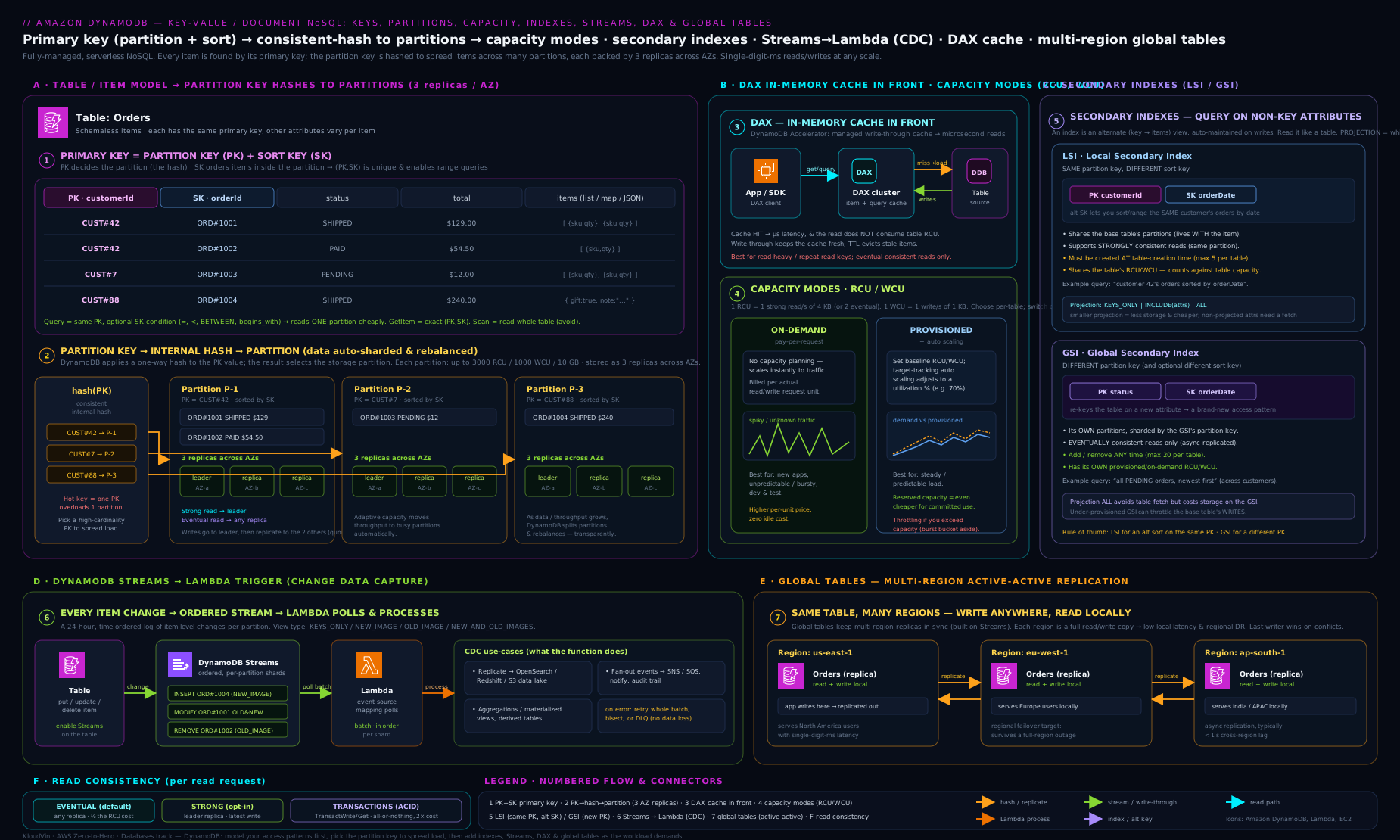
The diagram above ties the pieces together: items hashed by partition key onto partitions (with the sort key ordering items inside a partition), the two capacity modes feeding throughput, GSIs/LSIs as alternate query views, Streams emitting an ordered change log into Lambda/Kinesis (and powering global tables), DAX caching reads in front, and PITR/backups and KMS encryption wrapping the table — the same mental map to keep while you read the rest of this lesson.
Creating a table: every setting
Whether you use the console, CLI, or IaC, a table is defined by the same set of choices. Here is every one, with the what/choices/default/when/gotcha treatment.
| Setting | What it is / choices | Default | When / gotcha |
|---|---|---|---|
| Table name | Unique per Region per account | — | Immutable; choose a convention (app-env-entity) |
| Partition key | Name + type (S/N/B) — the hash key |
required | Immutable after creation; pick a high-cardinality value |
| Sort key | Optional name + type — the range key | none | Adds Query/range power; immutable; the combination must be unique |
| Capacity mode | On-demand or Provisioned | On-demand (console default) | Switchable once per 24 h; on-demand = safe default |
| Provisioned RCU/WCU | Throughput numbers (provisioned mode) | 5/5 (console) | Enable auto scaling with min/max + target % instead of fixing |
| Table class | Standard or Standard-IA (Infrequent Access) | Standard | Standard-IA: cheaper storage, pricier throughput — for large, rarely-read tables |
| Secondary indexes | LSIs (creation-time only) and GSIs (anytime) | none | LSIs share base capacity + 10 GB collection limit; GSIs have own capacity |
| Encryption | AWS owned / AWS managed / CMK | AWS owned | Always on; CMK for control + audit |
| DynamoDB Streams | Off, or on with a StreamViewType |
Off | Required for global tables & CDC; 24 h retention |
| Kinesis data stream | Optionally also stream to Kinesis | Off | For long retention / fan-out / analytics |
| TTL | Optional TTL attribute (Number, epoch seconds) | Off | Free deletes within ~48 h; deletions appear in Streams |
| PITR | Continuous backup (35-day restore) | Off (on by default for new tables in console as of recent updates) | Per-GB cost; restores to a new table |
| Deletion protection | Block accidental DeleteTable |
Off | Turn on for any production table |
| Tags | Key/value metadata | none | For cost allocation & governance |
Create a table with the CLI (composite key, on-demand, streams, PITR, deletion protection).
REGION=ap-south-1
aws dynamodb create-table \
  --table-name AppData \
  --attribute-definitions \
      AttributeName=PK,AttributeType=S \
      AttributeName=SK,AttributeType=S \
  --key-schema \
      AttributeName=PK,KeyType=HASH \
      AttributeName=SK,KeyType=RANGE \
  --billing-mode PAY_PER_REQUEST \
  --stream-specification StreamEnabled=true,StreamViewType=NEW_AND_OLD_IMAGES \
  --deletion-protection-enabled \
  --tags Key=env,Value=lab \
  --region $REGION
aws dynamodb wait table-exists --table-name AppData --region $REGION
aws dynamodb update-continuous-backups --table-name AppData \
  --point-in-time-recovery-specification PointInTimeRecoveryEnabled=true --region $REGION
Provisioned mode with auto scaling instead uses --billing-mode PROVISIONED --provisioned-throughput ReadCapacityUnits=5,WriteCapacityUnits=5, then aws application-autoscaling register-scalable-target + put-scaling-policy on dynamodb:table:ReadCapacityUnits/WriteCapacityUnits with a TargetTrackingScaling policy at 70%.
Add a GSI to a live table (any attribute, INCLUDE projection).
aws dynamodb update-table --table-name AppData \
  --attribute-definitions AttributeName=GSI1PK,AttributeType=S AttributeName=GSI1SK,AttributeType=S \
  --global-secondary-index-updates '[{"Create":{
      "IndexName":"GSI1",
      "KeySchema":[{"AttributeName":"GSI1PK","KeyType":"HASH"},{"AttributeName":"GSI1SK","KeyType":"RANGE"}],
      "Projection":{"ProjectionType":"INCLUDE","NonKeyAttributes":["status","total"]}}}]' \
  --region $REGION
The GSI back-fills in the background (the table stays available); watch IndexStatus go CREATING → ACTIVE.
After creation: what you can (and can’t) change
| Operation | Can you? | Notes |
|---|---|---|
| Change the partition/sort key | No | Keys are immutable — you must create a new table and migrate (export → transform → import). |
| Change capacity mode | Yes, once per 24 h | On-demand ⇄ provisioned. |
| Adjust provisioned RCU/WCU | Yes, anytime | Decreases are limited per day; auto scaling handles this for you. |
| Add/remove a GSI | Yes, anytime | Adding back-fills online; you can have GSIs in different states. |
| Add/remove an LSI | No | LSIs exist only from table creation. |
| Change a GSI’s projection | No | Delete and recreate the GSI with the new projection. |
| Enable/disable Streams | Yes (re-enabling starts a new stream, no history) | Required for global tables. |
| Enable/disable TTL, PITR, deletion protection | Yes, anytime | — |
| Change table class | Yes | Standard ⇄ Standard-IA. |
| Change encryption key | Yes | Switch among AWS-owned/managed/CMK. |
| Add a replica Region (global table) | Yes | Streams must be on; each replica billed separately. |
Hands-on lab
In this lab you create an on-demand table (so it costs essentially nothing), write and read items, run a Query, add a GSI, enable TTL, take a backup, and clean up. Uses the aws CLI (CloudShell or local).
1. Create an on-demand table with a composite key and a stream.
REGION=ap-south-1
aws dynamodb create-table --table-name LabOrders \
  --attribute-definitions AttributeName=PK,AttributeType=S AttributeName=SK,AttributeType=S \
  --key-schema AttributeName=PK,KeyType=HASH AttributeName=SK,KeyType=RANGE \
  --billing-mode PAY_PER_REQUEST \
  --stream-specification StreamEnabled=true,StreamViewType=NEW_AND_OLD_IMAGES \
  --region $REGION
aws dynamodb wait table-exists --table-name LabOrders --region $REGION
Expected: the wait returns once the table is ACTIVE.
2. Write a few items (two orders for one customer).
aws dynamodb put-item --table-name LabOrders --region $REGION --item '{
  "PK":{"S":"CUST#42"},"SK":{"S":"ORDER#2026-06-15#1001"},
  "status":{"S":"PLACED"},"total":{"N":"1299"},"city":{"S":"Mumbai"}}'
aws dynamodb put-item --table-name LabOrders --region $REGION --item '{
  "PK":{"S":"CUST#42"},"SK":{"S":"ORDER#2026-06-15#1002"},
  "status":{"S":"PLACED"},"total":{"N":"499"},"city":{"S":"Mumbai"}}'
Expected: both calls return with no error.
3. GetItem (one item by full key) and Query (all orders for the customer).
aws dynamodb get-item --table-name LabOrders --region $REGION \
  --key '{"PK":{"S":"CUST#42"},"SK":{"S":"ORDER#2026-06-15#1001"}}' \
  --consistent-read   # strongly consistent read

aws dynamodb query --table-name LabOrders --region $REGION \
  --key-condition-expression "PK = :c AND begins_with(SK, :p)" \
  --expression-attribute-values '{":c":{"S":"CUST#42"},":p":{"S":"ORDER#2026-06-15"}}' \
  --query "Items[].SK.S" --output table
Expected: the get-item returns the 1001 order (strongly consistent); the query returns both SKs in sort order — and note we used begins_with on the sort key, the canonical DynamoDB range pattern.
4. Add a GSI to query by status (a different access pattern), then query it.
aws dynamodb update-table --table-name LabOrders --region $REGION \
  --attribute-definitions AttributeName=status,AttributeType=S AttributeName=total,AttributeType=N \
  --global-secondary-index-updates '[{"Create":{
      "IndexName":"byStatus",
      "KeySchema":[{"AttributeName":"status","KeyType":"HASH"},{"AttributeName":"total","KeyType":"RANGE"}],
      "Projection":{"ProjectionType":"ALL"}}}]'
# wait for the GSI to finish back-filling:
aws dynamodb describe-table --table-name LabOrders --region $REGION \
  --query "Table.GlobalSecondaryIndexes[0].IndexStatus" --output text
# once it prints ACTIVE:
aws dynamodb query --table-name LabOrders --index-name byStatus --region $REGION \
  --key-condition-expression "#s = :v" \
  --expression-attribute-names '{"#s":"status"}' \
  --expression-attribute-values '{":v":{"S":"PLACED"}}' \
  --query "Items[].SK.S" --output table
Expected: IndexStatus transitions CREATING → ACTIVE; the GSI query returns both orders by status — an access pattern the base key could not serve. (Note GSI reads are eventually consistent — --consistent-read is rejected here.)
5. Enable TTL on an expiresAt attribute.
aws dynamodb update-time-to-live --table-name LabOrders --region $REGION \
  --time-to-live-specification "Enabled=true,AttributeName=expiresAt"
aws dynamodb describe-time-to-live --table-name LabOrders --region $REGION
Expected: TTL status ENABLED on expiresAt. (Items get deleted within ~48 h of their epoch timestamp passing — free of charge.)
6. Take an on-demand backup, then list it.
aws dynamodb create-backup --table-name LabOrders --backup-name LabOrders-snap --region $REGION
aws dynamodb list-backups --table-name LabOrders --region $REGION \
  --query "BackupSummaries[].{name:BackupName,status:BackupStatus}" --output table
Expected: a backup with status AVAILABLE.
7. Cleanup.
# delete the backup
BK=$(aws dynamodb list-backups --table-name LabOrders --region $REGION \
  --query "BackupSummaries[0].BackupArn" --output text)
aws dynamodb delete-backup --backup-arn "$BK" --region $REGION
# delete the table (this also removes its GSIs and stream)
aws dynamodb delete-table --table-name LabOrders --region $REGION
aws dynamodb wait table-not-exists --table-name LabOrders --region $REGION
Validation: aws dynamodb describe-table --table-name LabOrders --region $REGION eventually returns ResourceNotFoundException. (If delete-table is blocked, you left deletion protection on — aws dynamodb update-table --no-deletion-protection-enabled first.)
Cost note (INR-aware): an on-demand table with a handful of items and requests costs effectively nothing — DynamoDB’s free tier includes 25 GB of storage and a generous monthly allowance of on-demand requests, and you pay only per request beyond that. The things that quietly cost money: provisioned capacity left running (you pay per unit-hour even idle — which is why this lab used on-demand), GSIs with ALL projection (extra storage + a write per base write), PITR (per-GB), on-demand backups (persist until deleted — step 7 removes it), and a DAX cluster (always-on nodes). Deleting the table and the backup leaves nothing billing.
Going deeper
Everything so far is the model you need to use DynamoDB well. This section is the layer underneath — the mechanics that explain the surprises, plus the API details and patterns that separate a design that survives production from one that pages you at 2 a.m.
How partitions are really allocated (and why they never merge back)
You never manage partitions, but their arithmetic explains most throughput surprises. AWS historically published the model directly, and it still predicts behaviour. A table’s partition count is the larger of two pressures:
- By throughput:
ceil(provisionedRCU / 3000 + provisionedWCU / 1000)— because one partition tops out near 3,000 RCU and 1,000 WCU. - By size:
ceil(dataBytes / 10 GB)— because one partition holds roughly 10 GB.
Provisioned throughput is then split evenly across those partitions. Provision 9,000 RCU and DynamoDB spreads it over at least three partitions at ~3,000 each; if your traffic actually targets one key, that key still only gets its partition’s ~3,000, and you throttle at a third of the table’s headline capacity. That is the hot-partition problem stated arithmetically.
The gotcha that bites large, old tables: partitions split but never merge. Push a table to a huge provisioned number (or a big data size) and it acquires many partitions; scale the provisioned throughput back down and the partitions stay, so each now owns a smaller slice of the (now smaller) total — throughput dilution. A table that was fine at 40,000 WCU across 40 partitions can throttle at 4,000 WCU afterwards, because those same 40 partitions now share it at ~100 WCU each. Adaptive capacity softens all of this: DynamoDB continuously reallocates unused throughput toward busy partitions (within seconds now — “instant” adaptive capacity) and will isolate a single hot item onto its own partition. But adaptive capacity redistributes existing capacity; it cannot exceed a partition’s physical ceiling for one key, and it cannot fix a key whose every value is identical. On-demand hides the numbers entirely but obeys the same physics: it serves up to double your previous peak instantly and needs ~30 minutes to learn a new, higher one.
One distinction people conflate: the ~10 GB physical partition limit (DynamoDB simply splits when a partition fills, so a single partition-key value’s items can span many partitions) versus the 10 GB item-collection limit that applies only when a table has an LSI (there, one partition-key value’s items are hard-capped at 10 GB and cannot split). No LSI, no 10 GB cap on a key.
Pagination: the LastEvaluatedKey loop every caller must write
Query and Scan each return at most 1 MB of data per call — full stop, regardless of how many items match. If more exist, the response carries a LastEvaluatedKey, and you must call again passing it as ExclusiveStartKey to fetch the next page. A response with a LastEvaluatedKey is not “no more data”; a response without one means you have reached the end. The classic bug is reading the first page of a Query and treating it as the whole result — silently under-counting once the partition grows past 1 MB.
# page through a large partition with the CLI's built-in pagination tokens
aws dynamodb query --table-name AppData --region "$REGION" \
  --key-condition-expression "PK = :p" \
  --expression-attribute-values '{":p":{"S":"CUST#42"}}' \
  --max-items 100 --starting-token "$NEXT_TOKEN"   # omit --starting-token on the first call
The CLI’s --max-items/--starting-token/NextToken wrap the raw LastEvaluatedKey for you; the SDKs expose the raw key and most ship a paginator. Note that Limit (--page-size) caps items examined per page, not the total — it never removes the need to loop.
When a Scan is unavoidable: parallel Scan
Sometimes you genuinely must touch every item — a one-off backfill, an export, an ad-hoc analytics dump. A serial Scan reads 1 MB at a time from a single worker and crawls. Parallel Scan splits the table into TotalSegments logical slices and lets that many workers each Scan their own Segment concurrently:
# one of 10 workers (segments are 0-indexed: 0..9)
aws dynamodb scan --table-name AppData --region "$REGION" \
  --total-segments 10 --segment 3
Match TotalSegments to your worker count; each worker still paginates within its segment. It consumes read capacity fast (that’s the point), so rate-limit it or run it against on-demand so it does not starve production reads. Even so, prefer redesigning the access pattern into a Query or a sparse GSI (below) so a Scan never lands in the request path.
Optimistic locking with a version attribute
You rarely need a full transaction to make a single-item update safe against concurrent writers — a condition expression does it for a fraction of the cost. The pattern is optimistic locking: keep a numeric version attribute and only write if the version you read is still the one in the table.
aws dynamodb update-item --table-name AppData --region "$REGION" \
  --key '{"PK":{"S":"CUST#42"},"SK":{"S":"PROFILE"}}' \
  --update-expression "SET email = :e, version = version + :one" \
  --condition-expression "version = :v" \
  --expression-attribute-values '{":e":{"S":"new@x.io"},":one":{"N":"1"},":v":{"N":"7"}}'
If another writer bumped version to 8 first, your version = 7 check fails, the write is rejected with ConditionalCheckFailedException, and you re-read and retry. The same trick with attribute_not_exists(PK) turns a PutItem into a safe create-only (“claim a unique username”). High-level mappers automate it (e.g. the Java @DynamoDBVersionAttribute). A conditional write costs the same as a normal write when it succeeds and is still billed when the condition fails — so a hot retry loop burns WCUs.
Sparse and overloaded GSIs — how single-table design actually works
Two GSI tricks do most of the heavy lifting in real schemas:
- Sparse index. An item appears in a GSI only if it has that GSI’s key attributes. Set the GSI key attribute on only the items you want to find, and the index becomes a pre-filtered shortlist. Classic use: index only open tasks by writing an
openByattribute while a task is open and removing it on completion — aQueryon that GSI returns just the open tasks (no filter, noScan), and the index stays small and cheap because completed tasks are not in it. - Overloaded GSI. Give the index generic key names (
GSI1PK,GSI1SK) whose meaning differs per item type — for aUSERitemGSI1PKmight holdEMAIL#…, for anORDERitemSTATUS#…. One physical index then serves many unrelated access patterns, which is exactly how single-table designs keep the index count small (you get 20 GSIs per table by default). The single-table design lesson builds whole schemas this way.
Both patterns are why you model from access patterns: every new question is answered by a Query on a key or a sparse/overloaded GSI, never by scanning and filtering.
Tuning the Streams → Lambda event source mapping
When Lambda consumes a stream, the event source mapping (ESM) — not your function — controls throughput and failure handling, and its defaults are rarely what production wants:
BatchSize(up to 10,000 for streams) andMaximumBatchingWindowInSeconds(0–300) trade latency for fewer, larger invocations.ParallelizationFactor(1–10) runs that many concurrent invocations per shard while preserving per-partition-key order — the main lever to clear a backlog without adding shards.BisectBatchOnFunctionErrorsplits a failing batch in half and retries, so one poison record does not block the shard forever; pair it withMaximumRetryAttempts/MaximumRecordAgeInSecondsand an on-failure destination (SQS/SNS) so exhausted records are parked, not dropped.FilterCriterialets the ESM discard uninteresting records before they invoke Lambda (e.g. onlyeventName = MODIFY) — you pay nothing for filtered records, and it can cut invocations dramatically.
Because delivery is at-least-once and a retry re-delivers the whole batch, the consumer must be idempotent (dedupe on the item key plus the record’s sequence number). A cold, throttled, or slow consumer lets a shard’s records age toward the 24-hour cliff — watch the IteratorAge metric. The Streams CDC lesson and the Lambda performance lesson go deeper on both sides.
Multi-Region strong consistency (know the caveat)
The lesson states — correctly for the classic, default behaviour — that global tables are eventually consistent across Regions with last-writer-wins. AWS has since introduced an optional multi-Region strong consistency capability for global tables; treat it as an advanced, availability-limited option and confirm current support in your Regions before designing on it. The safe default remains: design for eventual cross-Region consistency, and if last-writer-wins is unacceptable, give each Region ownership of certain keys.
Costing it end to end (INR-aware)
The bill is just unit-counting. Take 50 M writes/month of ~1.5 KB items and 500 M eventually consistent reads/month of ~2 KB items, on-demand, with two ALL-projection GSIs:
- Writes: 1.5 KB rounds up to 2 write units per item → 100 M base; each
ALLGSI also gets every write → +200 M → 300 M write units. - Reads: 2 KB ≤ 4 KB, eventual = 0.5 read unit → 250 M read units.
At representative post-2024 us-east-1 on-demand rates (~$0.625 per million writes, ~$0.125 per million reads — AWS cut on-demand pricing ~50% in Nov 2024; verify your Region, ap-south-1 differs) that is ≈ $188 writes + $31 reads ≈ $219/month of throughput (~₹18–19k), before storage and PITR. The lesson in the numbers: the two ALL GSIs added 200 M of the 300 M write units — two-thirds of the write bill — which switching them to INCLUDE (only the attributes those queries return) would largely reclaim. Figures are representative; count your units and price them in the AWS calculator.
Common mistakes & troubleshooting
| Symptom | Likely cause | Fix |
|---|---|---|
ProvisionedThroughputExceededException / throttling on one key |
Hot partition from a low-cardinality or time-based partition key | Choose a high-cardinality key; write-shard skewed keys; rely on adaptive capacity for transient skew. |
| Throttling though total capacity looks fine (provisioned) | A single partition/key is the bottleneck, not the table total | Same as above; for steady spikes, switch to on-demand. |
| A query is slow and expensive and reads the whole table | You’re using Scan, not Query |
Redesign keys/indexes so the access pattern is a Query/GetItem; never Scan in a hot path. |
ValidationException: ... ConsistentRead ... not supported on ... index |
Asked for a strongly consistent read on a GSI | GSIs are eventually consistent only; drop --consistent-read or use an LSI/base table. |
| Writes to the base table suddenly throttle after adding a GSI | The GSI’s (provisioned) write capacity can’t keep up | Provision the GSI generously or use on-demand; project fewer attributes. |
| “I need to add an LSI but can’t” | LSIs are creation-time only | Use a GSI instead, or recreate the table with the LSI. |
| Query returns items missing some attributes | Those attributes aren’t projected into the GSI | Use INCLUDE (the needed attrs) or ALL projection; recreate the GSI to change projection. |
Item won’t save: Item size has exceeded the maximum |
Item exceeds the 400 KB limit | Store the large blob in S3, keep a pointer in DynamoDB; split the item. |
| TTL items still showing up | TTL deletes within ~48 h, not instantly; or wrong attribute type | Add a filter expression excluding expired items; ensure the TTL attribute is a Number epoch. |
| Cross-Region reads seem stale | Global tables are eventually consistent across Regions | Expected; design for it (last-writer-wins / Region-owned keys). |
Best practices
- Model from access patterns, not entities. List every query the app must serve first, then design keys and a small number of GSIs to make each one a
Query/GetItem— never aScan. (See the single-table design lesson.) - Pick a high-cardinality partition key and write-shard any naturally skewed (time-based, low-cardinality) key to avoid hot partitions.
- Default new workloads to on-demand; move to provisioned + auto scaling (and reserved capacity) only once traffic is steady and the per-request maths favours it.
- Project only what you query into GSIs (
INCLUDEoverALLwhere you can) to control write amplification and cost, and provision GSIs generously so they never throttle the base table. - Use eventually consistent reads by default (half the cost) and reserve strong reads for genuine read-after-write needs.
- Use TTL for expiring data (free deletes), DAX for read-heavy/hot-key/microsecond workloads, and transactions only when you genuinely need multi-item atomicity (they cost double).
- Turn on PITR and deletion protection for every production table; take on-demand backups before risky migrations; use global tables for multi-Region resilience and locality.
- Drive Streams from Lambda for CDC, make consumers idempotent, and choose
NEW_AND_OLD_IMAGESwhen you need to diff changes.
Security notes
- Encryption at rest is always on; use a customer-managed KMS key when you need rotation control, key policies, and the ability to revoke access (disabling the key disables the table). All API traffic is TLS.
- Authorise with least-privilege IAM scoped to specific table/index ARNs and actions; use
dynamodb:LeadingKeysfor fine-grained, per-item access (e.g. a user reads only their own partition) — the backbone of multi-tenant designs. - Restrict attributes where needed with the
dynamodb:Attributescondition and projection expressions so callers can’t read columns they shouldn’t. - Keep traffic private with a Gateway VPC endpoint for DynamoDB; there is no public database endpoint to lock down, but the endpoint keeps requests off the internet.
- Audit with CloudTrail — control-plane events always, and enable data events for sensitive tables to log item-level access.
- Lock down backups and exports (S3 export buckets) — they contain all your data; control who can
RestoreTable,ExportTableToPointInTime, and read the export bucket. - Beware
Scanin IAM-permissive roles — a broaddynamodb:Scanpermission can exfiltrate an entire table; grantQuery/GetIteminstead where possible.
Common beginner mistakes
These are not error messages — they are wrong mental models that lead you to design the error in. Each is a belief a beginner carries over from relational databases or picks up from the friendly console.
- “I’ll pick the keys later; any unique id will do.” The primary key is the one thing you can never change without rebuilding and migrating the table. Right model: list your access patterns first, then choose keys that make each one a
Query/GetItem. Keys are a consequence of your queries, not an afterthought. - “A
Scanwith a filter is basically aQuery.” A filter expression runs after the read — you pay to read (and are throttled by) every item scanned, and only then are the non-matching ones dropped. Right model: filters trim results, they never save capacity; make the key or a GSI select the items, and use filters only to shave a few edge cases off an already-narrowQuery. - “More GSIs, or
ALLprojection, can only help.” Every GSI is another table you write to on every relevant base write, andALLcopies the whole item into each. Right model: a GSI is a write-cost and storage multiplier — add the few you need and project only the attributes those queries return. - “Strongly consistent means globally consistent.” Strong reads are strong only within one Region and only on the base table or an LSI — never on a GSI, never across global-table Regions. Right model: “strong” answers “did my write land, here?”; GSI reads and cross-Region reads are always eventually consistent.
- “On-demand is the expensive mode, so I’ll switch to provisioned to save money.” Beginners flip a new, spiky table to provisioned and then either throttle or over-provision. Right model: on-demand is the safe default; provisioned only wins once traffic is steady enough to keep utilisation high — and even then you pair it with auto scaling.
- “TTL deletes at the exact second.” TTL is a background sweep that removes expired items within ~48 hours, not on the tick. Right model: store the epoch-seconds deadline for housekeeping, and if reads must look expired immediately, add a filter expression excluding past-TTL items.
- “The first page of a
Queryis the whole answer.” EveryQuery/Scanreturns at most 1 MB, then aLastEvaluatedKey. Right model: loop, passingLastEvaluatedKeyback asExclusiveStartKey, until it is absent — or you will silently under-read large partitions. - “I’ll bolt on an LSI when I need one.” LSIs exist only at table creation. Right model: if you might ever want an alternate strongly consistent sort order, decide at creation; otherwise reach for a GSI, which you can add to a live table.
- “DynamoDB has a database login like my SQL server.” There is no database user or password — every call is IAM-authorised. Right model: express access as least-privilege IAM policies on table/index ARNs, and use
dynamodb:LeadingKeysfor per-tenant, per-item isolation.
Interview & exam questions
-
What is the difference between a partition key and a sort key, and what does each enable? The partition key (hash key) determines which physical partition an item lives on (via an internal hash) and, alone, identifies an item in a simple primary key. Adding a sort key makes a composite key: items with the same partition key are stored together and sorted by sort key, which enables the efficient
Query(fetch a partition or a contiguous range). The partition key drives distribution; the sort key drives ordering/range within a partition. -
What causes a hot partition and how do you avoid it? Concentrating traffic on one (or few) partition-key values — a low-cardinality key, a time-based key (today’s date), or a single popular item. The table’s total capacity may be fine while one partition throttles. Avoid it with a high-cardinality partition key and by write-sharding skewed keys (suffix
#0..#N); adaptive capacity absorbs transient skew but can’t fix a fundamentally bad key. -
On-demand vs provisioned capacity — when each? On-demand scales automatically and you pay per request — best for spiky/unpredictable or new workloads and to avoid throttling from under-provisioning. Provisioned (with auto scaling and optionally reserved capacity) is cheaper per request for steady, predictable traffic if well-utilised, but you pay for provisioned units even when idle and can throttle when demand exceeds provisioned + burst. You can switch modes once per 24 h.
-
How do you compute RCUs and WCUs? 1 WCU = one 1 KB write/sec (round up; transactional = 2×). 1 RCU = one strongly consistent 4 KB read/sec, two eventually consistent 4 KB reads/sec (eventual = half), or one transactional read = 2 RCUs (round size up to 4 KB). E.g. a strongly-consistent read of an 8 KB item = 2 RCUs; eventually = 1 RCU.
-
LSI vs GSI — the key differences? An LSI shares the table’s partition key with a different sort key, must be created with the table, shares the base table’s capacity, supports strong reads, and is bound by the 10 GB item-collection limit. A GSI can use any attribute as its key, can be added/removed anytime, has its own capacity, is eventually consistent only, and has no collection-size limit. GSIs are the everyday tool; LSIs are for “same partition, alternate sort, strong read” cases.
-
What are index projections and why do they matter? A projection controls which attributes are copied into the index: KEYS_ONLY (keys only — smallest, may force a base-table follow-up read), INCLUDE (keys + named attributes — balanced), ALL (every attribute — convenient but largest, and you pay a full index write per base write). For a GSI, queries see only projected attributes. Choose
INCLUDEwith exactly what your queries return. -
What is a DynamoDB Stream and what are the StreamViewType options? An ordered, 24-hour log of item-level changes (create/update/delete) for CDC.
StreamViewTypeselects the payload: KEYS_ONLY, NEW_IMAGE, OLD_IMAGE, or NEW_AND_OLD_IMAGES (both — needed to diff). Ordering is guaranteed per partition key; delivery is at-least-once, so consumers (often Lambda via an event source mapping) must be idempotent. -
Eventual vs strong consistency — and where can’t you get strong? Eventual reads (default, half the cost) may briefly miss the latest write; strong reads (full cost, slightly higher latency, less resilient) always return the latest committed write. You cannot get a strong read on a GSI, and global tables are eventually consistent across Regions — “strong” is only ever within one Region.
-
What does DAX accelerate, and what can’t it do? DAX is a write-through, in-memory cache in front of DynamoDB that turns millisecond reads into microsecond reads for
GetItem/Query/Scan. It cannot serve strongly consistent reads (those bypass it) and doesn’t help write-heavy workloads; it runs as provisioned nodes in your VPC (always-on cost). -
How do DynamoDB transactions work and what do they cost?
TransactWriteItems/TransactGetItemsgive all-or-nothing ACID across up to 100 items/multiple tables in one Region. They cost double the normal capacity and can fail withTransactionCanceledExceptionon a failed condition or a conflict (retry). For single-item atomicity, a condition expression onPutItem/UpdateItemis cheaper. -
What is a global table and what consistency does it offer? A multi-Region, active-active replicated table (built on Streams) giving local low-latency reads/writes per Region and Region-level DR. Cross-Region replication is eventually consistent with last-writer-wins conflict resolution — so design for eventual consistency or give each Region ownership of certain keys.
-
PITR vs on-demand backups — when each? PITR continuously backs up and restores to any second in the last 35 days (great for “oops” recovery); on-demand backups are manual snapshots retained indefinitely for long-term/compliance needs. Both restore to a new table and don’t consume table capacity. For Region loss, use global tables, not backups.
Quick check
- You need every order for one customer, newest first, in one efficient call. What primary-key shape and which operation?
- True or false: you can add a Local Secondary Index to an existing table.
- A strongly-consistent read of a 10 KB item costs how many RCUs? Eventually consistent?
- Your GSI write capacity is too low in provisioned mode — what happens to writes on the base table?
- Which
StreamViewTypedo you choose when you need to compute exactly what changed on each update?
Answers
- A composite primary key (partition key =
customerId, sort key = something time/order-ordered likeORDER#<timestamp>), queried withQuery(optionally withScanIndexForward=falsefor newest-first). Same partition + sorted = one efficient range read. - False. LSIs can be created only at table creation; for an existing table use a GSI.
- 10 KB rounds up to 12 KB → 3 × 4 KB = 3 RCUs strongly consistent; eventually consistent is half, so 1.5 RCUs.
- The base table’s writes are throttled too — DynamoDB won’t let the GSI fall arbitrarily behind. Provision the GSI generously or use on-demand.
NEW_AND_OLD_IMAGES— it carries both the before and after item so the consumer can diff them.
Practice challenges
Six exercises, escalating from beginner to advanced. Try each before opening the solution; the one-line Why names the principle it exercises.
Challenge 1 — Pick the key shape (beginner). You must fetch a single user profile by userId, and you never query users any other way. What primary-key shape and which API call?
<details> <summary>Solution</summary>
A simple primary key (partition key = userId, no sort key), read with GetItem by that exact userId.
Why: a unique single-item lookup needs neither a sort key nor an index — anything more is capacity and complexity you will not use. </details>
Challenge 2 — Capacity-unit maths (beginner). For a 2.5 KB item, how many capacity units to (a) write it, (b) read it strongly, © read it eventually, (d) write it transactionally?
<details> <summary>Solution</summary>
(a) ceil(2.5 KB / 1 KB) = 3 WCU. (b) size rounds up to 4 KB → 1 RCU. © eventual = half → 0.5 RCU. (d) transactional write = 3 × 2 = 6 WCU.
Why: writes bill per 1 KB, reads per 4 KB; eventual is half a read, transactional is double — the four rules you forecast every bill with. </details>
Challenge 3 — Index and projection (intermediate). On a table keyed PK=CUST#id, SK=ORDER#ts, you must list all orders with status = SHIPPED, returning only orderId and total. Which index, key, and projection — and what is the risk in your chosen partition key?
<details> <summary>Solution</summary>
A GSI with partition key status and a sort key (e.g. ts), projection INCLUDE [total] (orderId already rides along as it is part of the base key). Query the GSI on status = SHIPPED. The risk: status is low-cardinality, so its GSI partition is a hot-partition candidate — mitigate by making the GSI key a composite like status#<shard> or scoping it by date (SHIPPED#2026-06).
Why: the base key cannot select by status; INCLUDE avoids both copying the whole item and a base-table follow-up read — but a low-cardinality index key reintroduces the hot-partition problem you solved on the base table.
</details>
Challenge 4 — Diagnose the throttle (intermediate). A table keyed on PK = eventDate (YYYY-MM-DD) throttles every day around a traffic spike, yet the consumed-vs-provisioned graphs show plenty of spare capacity. Why, and give two fixes.
<details> <summary>Solution</summary>
Today’s date is a single partition-key value, so all of today’s writes land on one partition (a hot “tail”) and throttle at that partition’s ceiling regardless of the table total. Fixes: (1) use a high-cardinality key such as eventId, with a GSI for date-range queries; (2) write-shard the date as YYYY-MM-DD#<0..N> and fan reads across the shards. Adaptive capacity absorbs transient skew but cannot rescue an all-same-value key.
Why: capacity limits are per partition, not per table — the headline number can look healthy while one key is saturated. </details>
Challenge 5 — Prevent a lost update (advanced). Two workers both read an item at version = 4 and both try to SET stock = stock - 1. Write the UpdateItem that prevents a lost update, and say what the loser sees.
<details> <summary>Solution</summary>
aws dynamodb update-item --table-name Inv --region "$REGION" \
  --key '{"PK":{"S":"SKU#9"}}' \
  --update-expression "SET stock = stock - :one, version = version + :one" \
  --condition-expression "version = :v" \
  --expression-attribute-values '{":one":{"N":"1"},":v":{"N":"4"}}'
The first write succeeds (version → 5). The second still asserts version = 4, which no longer holds, so it is rejected with ConditionalCheckFailedException; that worker re-reads (now version = 5, stock already decremented) and retries. A stock >= :one condition would additionally prevent overselling.
Why: the condition turns the update into a compare-and-swap on version, converting a silent lost update into a retryable conflict — optimistic locking without a transaction’s 2× cost.
</details>
Challenge 6 — Fan-out plus multi-Region (advanced). You need (a) every change fanned out to update a search index and (b) active-active writes in two Regions. Which stream setting, which consumer, and name one idempotency and one ordering caveat.
<details> <summary>Solution</summary>
Enable Streams with NEW_AND_OLD_IMAGES (global tables require it anyway). Drive the search index from a Lambda event source mapping (or an EventBridge Pipe / Kinesis Data Stream for longer retention and fan-out). Global tables (v2) replicate over those same streams — eventually consistent, last-writer-wins. Idempotency: dedupe on item key + sequence number, because delivery is at-least-once. Ordering: guaranteed only per partition key, not globally; and with two Regions the same item written in both resolves last-writer-wins, so the index may briefly reflect a superseded write.
Why: Streams power both CDC and cross-Region replication, but both are at-least-once and only per-key ordered — your consumer, not the stream, must supply exactly-once effect and tolerate reordering across keys. </details>
Exercise
Design the DynamoDB table(s) and indexes for a multi-tenant SaaS task tracker that must serve these access patterns: (a) get a single task by id; (b) list all tasks in a project, sorted by due date; © list all tasks assigned to a user across projects, filtered by status; (d) expire tasks 90 days after completion automatically; (e) react to every task change to update a per-project “open task count”. For each access pattern, state the key or index and the operation (GetItem/Query) you would use — and justify why none of them needs a Scan. Specify: the partition/sort key for the base table and how you avoid a hot partition for a very large project; the GSI(s) with their keys and projection (and why that projection); how you implement (d) with TTL; and how you implement (e) with Streams (which StreamViewType and why, and how you keep the consumer idempotent). Then choose a capacity mode with a one-line justification, and decide whether this design warrants DAX and/or a global table. Finally, write the aws dynamodb create-table and update-table (GSI) commands to build it.
Certification mapping
- AWS Certified Developer – Associate (DVA-C02): core territory — the data model and partition/sort keys,
QueryvsScan, LSI vs GSI and projections, RCU/WCU maths, eventual vs strong reads, DynamoDB Streams + Lambda triggers, transactions, conditional writes/optimistic locking, TTL, and DAX. - AWS Certified Solutions Architect – Associate (SAA-C03): when to choose DynamoDB vs RDS, on-demand vs provisioned (+ auto scaling), GSIs for access patterns, global tables for multi-Region, DAX for read acceleration, PITR/backup, and encryption.
- AWS Certified SysOps Administrator – Associate (SOA-C02): operating tables — capacity/auto scaling, CloudWatch metrics (
ThrottledRequests,ConsumedRead/WriteCapacityUnits), PITR/backups, and adaptive-capacity/hot-partition troubleshooting. - AWS Certified Solutions Architect – Professional / Data Engineer: deeper modelling (single-table design), Streams/Kinesis CDC pipelines, global-table conflict design, and cost optimisation (reserved capacity, table classes, projection tuning).
Glossary
- Table / item / attribute — a collection of items; an item is a set of attributes (name/value); the only shared structure is the primary key.
- Partition key (hash key) — the attribute hashed to choose an item’s partition; drives data distribution.
- Sort key (range key) — the second part of a composite key; orders items within a partition and enables
Queryranges. - Partition — an internal storage unit (≈10 GB, ~3,000 RCU / ~1,000 WCU) replicated across 3 AZs; tables grow by adding partitions.
- Hot partition — a partition receiving disproportionate traffic (from a skewed key), causing throttling despite spare table capacity.
- RCU / WCU — read/write capacity units: 1 RCU = one strong 4 KB read/s (or two eventual); 1 WCU = one 1 KB write/s.
- On-demand / provisioned — pay-per-request auto-scaling mode vs pre-provisioned throughput (with auto scaling/reserved capacity).
- LSI / GSI — Local (same PK, alt sort, creation-time, shares capacity, strong reads) / Global (any key, anytime, own capacity, eventual) Secondary Index.
- Projection — which attributes an index copies: KEYS_ONLY, INCLUDE, or ALL.
- DynamoDB Stream — ordered 24-h change log (per-partition order);
StreamViewType= KEYS_ONLY / NEW_IMAGE / OLD_IMAGE / NEW_AND_OLD_IMAGES. - TTL — automatic, free deletion of items past an epoch-seconds timestamp attribute (within ~48 h).
- DAX — DynamoDB Accelerator, a managed in-memory write-through read cache (microsecond reads; no strong reads).
- Transaction —
TransactWriteItems/TransactGetItems: ACID across ≤100 items in one Region, at 2× capacity cost. - Eventual vs strong consistency — default half-cost reads that may lag vs full-cost reads of the latest write (no strong on GSIs/across Regions).
- Global table — a multi-Region, active-active replicated table (eventually consistent, last-writer-wins).
- PITR — point-in-time recovery: restore to any second in the last 35 days (to a new table).
- Adaptive capacity — DynamoDB automatically shifting throughput toward busy partitions (and isolating a single hot item), which absorbs transient skew but cannot rescue a fundamentally low-cardinality key.
- Write sharding — spreading a naturally skewed key across
key#0..key#Nsuffixes so writes fan out over many partitions instead of one hot one. - Item collection — all items sharing one partition-key value (across the base table and its LSIs); hard-capped at 10 GB only when the table has an LSI.
- Sparse index — a GSI that indexes only items which have its key attribute, giving a pre-filtered shortlist (e.g. only “open” items) with no scan.
- Overloaded GSI — a GSI with generic key names (
GSI1PK/GSI1SK) whose meaning varies by item type, so one index serves many access patterns. - Condition expression / optimistic locking — a predicate attached to a write that must hold or the write is rejected with
ConditionalCheckFailedException; comparing-and-swapping aversionattribute this way is optimistic locking. - Query vs Scan —
Queryreads one partition by key (optionally a sort range) cheaply;Scanreads the whole table/index and then filters — avoid it in hot paths. - Pagination (
LastEvaluatedKey) —Query/Scanreturn ≤ 1 MB per call; a returnedLastEvaluatedKey, passed back asExclusiveStartKey, means “more pages remain”. - Parallel Scan — splitting a
ScanintoTotalSegmentsslices read by concurrent workers (each its ownSegment) for one-off full-table jobs. - Burst capacity — up to ~5 minutes of unused provisioned throughput banked to absorb short spikes before throttling begins.
Next steps
You now know DynamoDB end to end — the data model and partition/sort keys, how partitioning and hashing cause and prevent hot partitions, both capacity modes and the RCU/WCU maths, LSIs vs GSIs and projections, Streams and CDC, TTL, DAX, transactions, the consistency model, global tables, and PITR/backups/encryption. From here:
- Turn this into real schemas with DynamoDB Single-Table Design: Modeling Access Patterns, GSIs, and Hot Partition Avoidance.
- Build reliable event-driven pipelines off the change log in Change Data Capture with DynamoDB Streams: Lambda Triggers, EventBridge Pipes, and Exactly-Once Processing.
- Next in the course we move from the data store to the API in front of it: Amazon API Gateway, In Depth: REST vs HTTP vs WebSocket APIs, Integrations & Authorizers.