In a nutshell
An enterprise big-data platform is the machinery that takes every messy stream and file a company produces and turns it into one trustworthy, fast-to-query, ML-ready source of truth — so three teams stop computing “active customer” three different ways. This lesson is a complete, reusable reference architecture for that platform on Google Cloud, built from the services that actually do the heavy lifting: Cloud Storage (the lake), Dataproc and Dataflow (the two processing engines), BigQuery (the warehouse and serving surface), Cloud Composer (the orchestrator), and Dataplex (governance).
The mental model that makes all the parts click is a city water system, not a single pipe. Rain and rivers arrive dirty and unpredictable — that is your clickstream, point-of-sale drops, database change-feeds, and third-party files. A utility turns that into safe water at the tap with a handful of moving parts this platform mirrors exactly:
- A huge, cheap reservoir that stores raw water first and asks questions later — that is the Cloud Storage data lake, your durable system of record, priced so you can afford to keep everything.
- Treatment stages — coarse screening, settling, filtration, final polish — so water gets cleaner in named steps you can inspect — that is the raw → curated → consumption (bronze/silver/gold) zone discipline, and it is what stops a lake becoming a swamp.
- Two pumping systems: high-pressure mains for firefighting right now (the streaming path — Dataflow off Pub/Sub) and the scheduled bulk works that refill the reservoir overnight (the batch path — Dataproc Spark). One clock is never enough.
- One distribution network everyone drinks from, where “clean” is defined exactly once — that is BigQuery, the single query surface for dashboards, analysts, and ML, so nobody bottles their own private supply.
- A control room scheduling every pump and valve — Cloud Composer (Airflow) — plus a water-quality lab, meters, and locked access — Dataplex, Sensitive Data Protection, IAM, and VPC Service Controls — so the water is safe, measured, and only reaches who’s allowed.
Get that shape right once and adding the next source or the next consumer is cheap, because storage, compute, serving, and governance each scale on their own. That is the whole promise of a real data platform: many noisy inputs, one governed, query-fast, cost-predictable output — and no lock-in to a single processing engine.
Level: Advanced · Time: ~40 min
Before you start — and what you’ll walk away with
This is an architecture-level lesson: it wires many services into one platform rather than teaching any single one from zero. It assumes you have met the big building blocks at least in passing. If any feels unfamiliar, skim these first:
- Dataflow deep dive: Apache Beam, streaming & batch — the streaming engine and the unified batch/stream model.
- BigQuery deep dive: datasets, partitioning, slots & pricing — the warehouse, and the partition/cluster/slot levers this design leans on hardest.
- Pub/Sub deep dive: topics, subscriptions & delivery — the streaming front door and its delivery guarantees.
- The GCP lakehouse pattern in depth — the open-format lake-plus-warehouse pattern this architecture is a superset of.
After working through it you will be able to:
- Draw the end-to-end platform — ingestion (batch + stream) → lake zones → two engines → warehouse → serving — and say in one sentence what each stage exists to remove.
- Choose the right engine and clock per job — Dataflow (Beam) vs Dataproc (Spark), streaming vs batch — instead of forcing everything through one.
- Partition and cluster a BigQuery table so a runaway
SELECTcan’t scan a terabyte, and explain why bytes-scanned is the master cost lever. - Lay out the lake as raw → curated → consumption with open-format Iceberg/Parquet, and know when to query in place (BigLake) versus load native.
- Make the warehouse rebuildable from the lake as your real disaster-recovery posture, and reason about RTO/RPO per data tier.
- Hold the cost line — serverless compute that scales to zero, storage tiering, Spot workers, slots-vs-on-demand — and defend each choice to a budget-conscious sponsor.
Every enterprise eventually hits the same wall: the data exists, but it is trapped. Sales sits in a CRM, clickstream lands in an event bus, the warehouse holds yesterday’s truth, and a dozen CSV exports rot in shared drives. Analysts wait days for a number, data scientists copy production tables to laptops, and nobody trusts the dashboard because three teams compute “active customer” three different ways. This article is a complete, reusable GCP architecture for big data processing — the kind of platform that takes raw events and files in at one end and produces governed, query-ready, ML-ready data at the other. It is built on the services that actually do the heavy lifting on Google Cloud: Cloud Storage as the lake, Dataproc for Spark/Hadoop workloads, Dataflow for streaming and unified batch pipelines, BigQuery as the serverless warehouse and serving layer, and Cloud Composer (managed Apache Airflow) as the orchestration brain.
The business scenario
Picture a mid-market retailer — call the pattern “RetailCo” for now; we will name a concrete company later. They run e-commerce plus 140 physical stores. Their data problem is not exotic, which is exactly why this architecture is widely useful:
- Volume and variety. ~3 TB/day of new data: web/app clickstream (JSON events on Pub/Sub), point-of-sale transactions (hourly CSV/Parquet drops from stores), product catalog and inventory (relational, change-data-capture), and third-party feeds (weather, ad spend, market basket benchmarks) arriving as files.
- Two clocks. The business needs real-time signals (fraud scoring, live inventory, “trending now” merchandising) and batch truth (nightly revenue, cohort retention, finance reconciliation, ML training sets). One clock is not enough.
- Heterogeneous compute. The data-engineering team already has thousands of lines of Apache Spark (PySpark and Spark SQL) and some legacy Hive jobs. The analytics team lives in SQL. The ML team wants notebooks and feature tables. A good platform serves all three without forcing a rewrite.
- Governance is now mandatory. PII (emails, addresses, payment tokens) flows through the system. Auditors, GDPR/CCPA, and PCI scope mean access must be least-privilege, lineage must be traceable, and sensitive columns must be discoverable and masked.
- Cost is watched. This is not a hyperscaler with an infinite budget. Leadership has seen “data platform” projects balloon, so every design choice must justify itself, and idle infrastructure is the enemy.
The same shape applies to a fintech (transactions + risk), a media company (impressions + content analytics), a manufacturer (IoT telemetry + ERP), or a SaaS vendor (product usage + billing). Small enterprises run a trimmed version (one region, autoscaling to zero); large enterprises run the full multi-zone, multi-project, governed version. The architecture scales down as gracefully as it scales up, which is the test of a real reference design.
The problem this solves, stated plainly: turn many noisy sources into one governed, query-fast, cost-predictable data platform that serves real-time, analytical, and ML consumers from the same source of truth — without locking you into a single processing engine.
Architecture overview
The platform is a lakehouse: a Cloud Storage data lake for cheap, open-format storage, fronting BigQuery as the warehouse and serving engine, with Dataproc and Dataflow as the two complementary processing engines and Composer conducting the whole orchestra. Data flows through medallion-style zones — raw → curated → consumption (bronze/silver/gold).
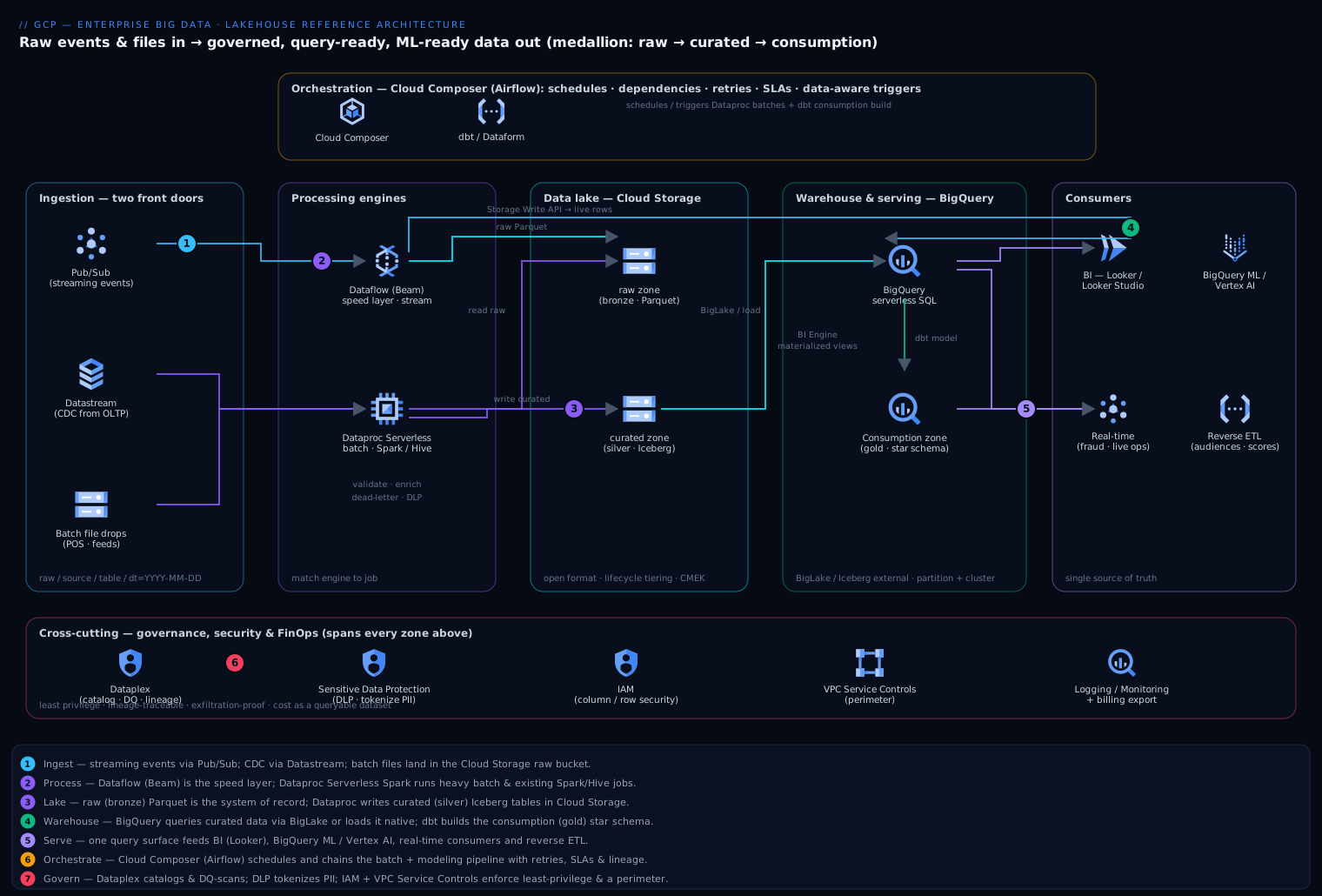
Read the diagram as a river flowing left to right. Messy sources enter through two front doors on the left — a streaming door (Pub/Sub) and a batch door (files landing in Cloud Storage). The two engines in the middle — Dataflow for streams, Dataproc for Spark batch — treat the water through the raw → curated → consumption zones of the lake. BigQuery on the right is the single tap every consumer drinks from: BI, ad-hoc SQL, BigQuery ML and Vertex AI. Wrapping the whole estate, Cloud Composer conducts the schedule while Dataplex, DLP, IAM and VPC Service Controls govern and guard it.
End-to-end data path:
-
Ingestion. Two front doors. Streaming events (clickstream, app telemetry, CDC) publish to Pub/Sub. Batch files (POS drops, third-party feeds, exports) land in a Cloud Storage
rawbucket, organized asraw/<source>/<table>/dt=YYYY-MM-DD/. CDC from operational databases uses Datastream, which writes change records into therawbucket (and can target BigQuery directly). -
Stream processing. A Dataflow streaming pipeline (Apache Beam) subscribes to Pub/Sub, validates and enriches events, dead-letters bad records, and writes two ways: low-latency rows into BigQuery via the Storage Write API (for live dashboards and fraud features) and raw-but-structured Parquet into Cloud Storage
raw(so the lake remains the complete system of record). This is the speed layer. -
Batch transformation. Cloud Composer (Airflow) orchestrates the batch layer. On schedule (or triggered by file arrival), it runs Dataproc Serverless Spark jobs that read the
rawzone, clean/conform/deduplicate, apply business logic and SCD (slowly changing dimension) handling, and write curated data as partitioned, Apache Iceberg-managed Parquet in Cloud Storage. Heavy ML feature engineering and any existing PySpark/Hive workloads run here too — Dataproc gives the team their familiar Spark engine without managing clusters. -
Warehouse load and modeling. Curated tables are exposed to BigQuery either as BigLake external/Iceberg tables (query in place, no copy) or loaded as native BigQuery tables when query performance demands it. Composer then runs dbt (or BigQuery scheduled SQL) to build the consumption zone: star schemas, conformed dimensions, aggregate/rollup tables, and the metrics layer where “active customer” is defined exactly once.
-
Serving and consumption. BigQuery is the single query surface. BI (Looker / Looker Studio) reads consumption tables; ad-hoc analysts query with SQL and BI Engine for sub-second dashboards; ML uses BigQuery ML for in-warehouse models and Vertex AI for heavier training, reading curated feature tables; reverse ETL pushes audiences and scores back to operational systems. Real-time consumers (fraud service, live ops) read the freshly-streamed BigQuery tables.
-
Cross-cutting. Dataplex provides the data-mesh governance fabric — it catalogs every asset across the buckets and datasets, runs data-quality and data-profiling scans, and applies policy. Cloud DLP / Sensitive Data Protection discovers and classifies PII. IAM + VPC Service Controls enforce access and create a perimeter so data cannot be exfiltrated. Cloud Logging/Monitoring observes pipeline health, and billing exports to BigQuery make cost itself a queryable dataset.
The mental model: Cloud Storage is the durable floor, BigQuery is the serving ceiling, Dataproc and Dataflow are the two engines (batch-heavy/Spark and streaming/Beam respectively), and Composer is the conductor. Each can be adopted incrementally.
Component breakdown
| Component | GCP service | Role in this architecture | Key configuration choices |
|---|---|---|---|
| Data lake | Cloud Storage | System of record for raw + curated open-format data | Dual-region or regional buckets; lifecycle to Nearline/Coldline/Archive; uniform bucket-level access; CMEK; hierarchical namespace for analytics |
| Streaming ingest | Pub/Sub | Decoupled, durable event intake | Topic per domain; dead-letter topic; schema enforcement; 7-day retention for replay; ordering keys where needed |
| CDC ingest | Datastream | Change-data-capture from OLTP databases | Stream to Cloud Storage and/or BigQuery; backfill + ongoing CDC; private connectivity |
| Stream/unified processing | Dataflow (Apache Beam) | Speed layer: validate, enrich, window, dead-letter | Streaming Engine on; autoscaling + Dataflow Prime; exactly-once to BigQuery via Storage Write API; Flex Templates for CI/CD |
| Batch/Spark processing | Dataproc Serverless + Dataproc on GCE | Heavy transforms, Iceberg writes, existing Spark/Hive, ML features | Serverless batches as default (autoscale, pay-per-job); persistent clusters only for interactive/Hive; Spot/preemptible secondary workers; PHS (Persistent History Server) |
| Warehouse + serving | BigQuery | Serverless SQL warehouse, serving + ML layer | Editions (Standard/Enterprise) with autoscaling slots + reservations; partitioning + clustering; BI Engine; materialized views; BigLake/Iceberg external tables |
| Orchestration | Cloud Composer (Airflow) | Schedules, dependencies, retries, SLAs across the pipeline | Composer 2 (GKE Autopilot, env autoscaling); deferrable operators; DAG-as-code in Git; data-aware (dataset) triggering |
| Transformation framework | dbt (on Composer or Dataform) | Declarative SQL modeling of the consumption zone | Tests + docs + lineage; incremental models; one metrics definition |
| Governance fabric | Dataplex | Catalog, data quality, profiling, lakes/zones, lineage | Lakes map to domains; auto-discovery of GCS + BQ; DQ scans gate publishing; built-in lineage |
| Data protection | Sensitive Data Protection (DLP) | Discover, classify, de-identify PII | Inspection templates; de-identification (tokenization/masking) in Dataflow; column-level findings into Dataplex |
| Access control | IAM + VPC Service Controls | Least-privilege + exfiltration perimeter | Custom roles; BigQuery column/row-level security + policy tags; service perimeter around analytics projects |
A few component choices deserve the “why,” because they are the decisions that separate a real architecture from a sketch:
Why both Dataproc and Dataflow, not one? They solve different problems and overlap less than it looks. Dataflow (Beam) is the right tool for streaming and for unified pipelines authored once and run in both modes; it is fully serverless, autoscales aggressively, and gives exactly-once semantics into BigQuery. Dataproc is the right tool when you have existing Spark/Hadoop/Hive assets, need specific Spark libraries (Delta/Iceberg, GeoSpark, Spark MLlib), or run heavy batch transforms where Spark’s ecosystem and the team’s existing skills win. Forcing all batch into Beam would mean rewriting thousands of tested PySpark lines; forcing streaming into Spark Structured Streaming on a standing cluster would mean paying for idle nodes and managing them. Use the engine that fits the job.
Why Dataproc Serverless as the default, not standing clusters? Standing clusters bill for every minute whether or not a job runs — the classic way data-platform costs balloon. Dataproc Serverless for Spark spins up per-batch, autoscales, and tears down, so you pay for compute you actually use. Keep a small persistent cluster only for interactive notebooks or Hive metastore-heavy interactive work; everything scheduled goes serverless. Add Spot/preemptible secondary workers for fault-tolerant batch to cut compute cost dramatically.
Why a lakehouse with Iceberg and BigLake instead of “just load everything into BigQuery”? Two reasons. First, open format = no lock-in and one copy: curated data lives as Iceberg/Parquet in Cloud Storage and is queryable by BigQuery (via BigLake), by Spark on Dataproc, and by external engines — without duplicating it per consumer. Second, cost tiering: cold raw data sits on cheap object storage with lifecycle rules, while only the hot serving tables get BigQuery’s premium engine. You load into native BigQuery selectively, where query latency justifies it.
Why BigQuery partitioning + clustering matters so much. BigQuery on-demand pricing charges by bytes scanned. A fact table partitioned by event date and clustered by customer_id/product_id lets the engine prune to a single day and a few clusters, turning a multi-TB scan into a few GB. This single configuration choice is often the largest lever on both query cost and speed.
Why Composer over Cloud Scheduler + Functions. Real pipelines have dependencies (don’t build gold before silver), retries with backoff, backfills, SLAs, and data-aware triggers (run when a partition lands). Airflow expresses all of this as code in Git, with a UI for operators. Composer 2 runs it on autoscaling GKE Autopilot so the orchestrator itself isn’t a cost or ops burden.
Implementation guidance
Project and environment topology. Use a multi-project layout under a folder per environment (dev/stage/prod), provisioned with a landing-zone/Terraform foundation:
prj-data-ingest— Pub/Sub topics, Datastream, ingestion Dataflow jobs, raw bucket.prj-data-lake— Cloud Storagerawandcuratedbuckets, Dataproc, BigLake connections, Dataplex lakes.prj-data-warehouse— BigQuery datasets (curated, consumption), BI Engine, reservations.prj-data-orchestration— Cloud Composer environment, dbt, CI/CD service accounts.prj-data-governance(often the host project) — Dataplex, DLP templates, central log sink, billing export dataset.
This separation lets you scope IAM and VPC Service Controls per blast-radius and bill per domain. A small enterprise can collapse these into one or two projects; the IAM and perimeter patterns still hold.
Infrastructure as Code. Terraform is the natural fit on GCP (Deployment Manager is legacy; Config Connector/Crossplane are options for GitOps-on-GKE shops). Use the Google Cloud Foundation Fabric modules and the resource-specific Terraform modules. Concretely:
google_storage_bucketwithuniform_bucket_level_access,lifecycle_rule(transition raw to Nearline at 30 days, Coldline at 90, Archive at 365),encryption(CMEK from Cloud KMS), andsoft_delete_policy.google_pubsub_topic+google_pubsub_subscriptionwithdead_letter_policyand a schema (google_pubsub_schema).google_dataproc_batchfor serverless Spark jobs (orgoogle_dataproc_clusterfor the small persistent cluster) referencing an image version and a Persistent History Server.google_dataflow_flex_template_job(or the Flex Template launcher) so streaming pipelines deploy from a container image via CI/CD, withenable_streaming_engine = true.google_bigquery_datasetandgoogle_bigquery_tablewithtime_partitioning,clustering,require_partition_filter = true, and column-levelpolicy_tags.google_bigquery_reservation+google_bigquery_capacity_commitmentfor predictable warehouse capacity, plus on-demand for spiky workloads.google_composer_environment(Composer 2) sized with environment autoscaling; DAGs deployed from Git via Cloud Build syncing to the Composer DAGs bucket.google_dataplex_lake/_zone/_assetmapping domains to buckets and datasets;google_data_loss_prevention_inspect_templatefor DLP.
Keep pipeline code (Beam pipelines, PySpark jobs, dbt models, Airflow DAGs) in application repos, separate from infrastructure Terraform. CI/CD: Cloud Build (or GitHub Actions) builds Dataflow Flex Template images, packages Spark jobs to GCS, runs dbt build against a CI dataset, and validates/uploads DAGs. Promote artifacts dev → stage → prod; never click-deploy pipelines.
Networking. Run all processing with private connectivity: a Shared VPC with Private Google Access so Dataflow/Dataproc workers have no external IPs. Use Private Service Connect / private endpoints for BigQuery and other APIs. Datastream to on-prem or other-cloud databases uses private connectivity (VPC peering or PSC). Egress is constrained by firewall rules and, crucially, by VPC Service Controls — a service perimeter around the analytics projects means even a leaked credential cannot copy BigQuery data to a bucket outside the perimeter. Place a single egress point with Cloud NAT for the rare cases workers must reach the internet (third-party APIs), and log it.
Identity wiring. Every pipeline runs as a dedicated, least-privilege service account — separate SAs for ingestion Dataflow, Dataproc batches, Composer, and dbt. Grant narrow predefined or custom roles (e.g., Composer’s SA gets roles/dataproc.editor and roles/bigquery.jobUser but not broad storage admin). Human access is via Google Groups mapped to IAM roles, ideally federated from your IdP through Workforce Identity Federation so there are no standalone Google passwords. For cross-cloud or CI systems, use Workload Identity Federation instead of exported SA keys (keys are the most common leak vector — avoid them entirely). In BigQuery, enforce column-level security via policy tags on PII columns and row-level security for tenant/region isolation, so the same table serves many audiences safely.
The decisions in code
The prose above states the rules; the snippets below show what a few of the load-bearing decisions look like in code. Every command and block is real and current — treat the placeholder IDs (project, bucket, connection, and service-account names) as your own.
Tier the lake automatically (Terraform). The raw zone is written once and read rarely after a week, so lifecycle rules demote it down the storage classes without anyone touching it — the cost-tiering this architecture depends on:
resource "google_storage_bucket" "raw" {
  name                        = "northwave-data-raw"      # globally unique
  location                    = "US"                       # multi-region → geo-redundant
  storage_class               = "STANDARD"
  uniform_bucket_level_access = true                       # IAM only, no legacy ACLs
  force_destroy               = false

  versioning {
    enabled = true                                         # protect against bad overwrites
  }

  lifecycle_rule {
    condition { age = 30 }
    action {
      type          = "SetStorageClass"
      storage_class = "NEARLINE"
    }
  }
  lifecycle_rule {
    condition { age = 90 }
    action {
      type          = "SetStorageClass"
      storage_class = "COLDLINE"
    }
  }
  lifecycle_rule {
    condition { age = 365 }
    action {
      type          = "SetStorageClass"
      storage_class = "ARCHIVE"
    }
  }

  encryption {
    default_kms_key_name = "projects/prj-data-lake/locations/us/keyRings/data/cryptoKeys/gcs"
  }
}
Make bytes-scanned small (BigQuery DDL). On-demand BigQuery bills by bytes scanned, so partitioning by date and clustering by the common filter keys is the single biggest lever on both cost and speed. require_partition_filter makes it impossible to forget:
CREATE TABLE consumption.fct_orders (
  order_id     STRING,
  customer_id  STRING,
  product_id   STRING,
  store_id     STRING,
  order_ts     TIMESTAMP,
  gross_amount NUMERIC
)
PARTITION BY DATE(order_ts)
CLUSTER BY customer_id, product_id
OPTIONS (
  require_partition_filter  = TRUE,
  partition_expiration_days = 1825   -- drop partitions older than 5 years
);
A query that respects both prunes a multi-terabyte table down to a few gigabytes:
SELECT customer_id, SUM(gross_amount) AS revenue
FROM consumption.fct_orders
WHERE order_ts >= TIMESTAMP('2026-07-01')     -- partition prune: 7 days, not all history
  AND order_ts <  TIMESTAMP('2026-07-08')
  AND customer_id = 'C-000123'                -- cluster prune: a few blocks, not the whole day
GROUP BY customer_id;
Run Spark without a standing cluster (Dataproc Serverless). Existing PySpark runs unchanged; the batch spins up, autoscales, and tears down, so you pay only for the job. A Persistent History Server keeps the Spark UI available after the batch is gone:
gcloud dataproc batches submit pyspark \
  gs://PLACEHOLDER-CODE/jobs/conform_pos.py \
  --project=prj-data-lake \
  --region=us-central1 \
  --version=2.2 \
  --subnet=projects/prj-host/regions/us-central1/subnetworks/data-subnet \
  --service-account=sa-dataproc-batch@prj-data-lake.iam.gserviceaccount.com \
  --history-server-cluster=projects/prj-data-lake/regions/us-central1/clusters/phs \
  --properties=spark.dynamicAllocation.enabled=true \
  -- --run-date=2026-07-18
Query the curated zone in place (BigLake + Iceberg). Curated data lives once as Iceberg/Parquet in GCS, and BigQuery reads it without a copy — Spark on Dataproc reads the same table. No duplication per consumer, no lock-in:
CREATE EXTERNAL TABLE curated.orders
WITH CONNECTION `prj-data-lake.us.biglake`
OPTIONS (
  format = 'ICEBERG',
  uris   = ['gs://northwave-curated/orders/metadata/v3.metadata.json']
);
Notice the through-line: each snippet is a cost or governance decision, not just a resource. Tiering, pruning, scale-to-zero, and query-in-place are the four habits that keep this platform fast and affordable.
Enterprise considerations
Security and Zero Trust. Zero Trust here means no implicit trust by network location and least privilege everywhere. The pillars: (1) No SA keys — federation only. (2) VPC Service Controls perimeter so identity and context (device, origin) gate access and exfiltration is structurally blocked. (3) Private-only data plane — no public IPs on workers, private API access. (4) CMEK on buckets, BigQuery, and Dataproc/Dataflow temp storage, with keys in Cloud KMS you control and can rotate/revoke. (5) PII handled at ingest — the Dataflow pipeline calls Sensitive Data Protection to tokenize/mask emails and payment data before they reach curated tables; raw sensitive data is access-restricted and short-lived. (6) Column- and row-level controls in BigQuery via policy tags. (7) Audit everything — Cloud Audit Logs (Data Access logs on BigQuery) exported to a locked, separate log project. A hard lesson worth stating: never commit credentials to Git, and if a secret ever lands in history, rotate it immediately rather than just deleting the file — git history is forever.
Cost optimization. This architecture is deliberately cost-defensive:
- Compute that scales to zero. Dataproc Serverless and Dataflow autoscaling mean no idle cluster bills. Standing infrastructure is minimized to a small interactive cluster and the (autoscaling) Composer environment.
- Spot/preemptible secondary workers for fault-tolerant Spark batch — large savings on the heaviest jobs.
- Storage tiering via lifecycle rules: most raw data is read once after a week, so it drops to Nearline/Coldline/Archive automatically.
- BigQuery: the two biggest levers. Partition + cluster every large table and set
require_partition_filterso a runaway query can’t scan a year. Choose pricing deliberately — on-demand (per-TB scanned) for spiky/unpredictable workloads, Editions with autoscaling slots + capacity commitments for steady high-volume workloads (commitments cut the rate). Use materialized views and BI Engine to avoid re-scanning for dashboards. - FinOps as data. Export billing to BigQuery and build a cost dashboard with per-pipeline labels; set budgets and alerts; review the most expensive queries weekly. Cost is a dataset you query like any other.
Scalability. Each tier scales independently. Pub/Sub absorbs traffic spikes with buffering; Dataflow Streaming Engine adds workers under load; Dataproc Serverless sizes per batch; BigQuery’s serverless slots scale to thousands of concurrent queries. The lake (Cloud Storage) is effectively unbounded. Because storage and compute are separate, you scale the expensive part (compute) only when running, and grow the cheap part (storage) freely. The design that serves 3 TB/day serves 30 TB/day by changing autoscaling ceilings and slot reservations — not by re-architecting.
Reliability and DR (RTO/RPO). Set targets by data tier:
- Streaming front door (RPO near zero, RTO minutes): Pub/Sub retains messages (7-day retention + dead-letter) so a downstream outage loses nothing — you replay. Dataflow checkpoints; jobs restart from the last commit. Run regional services; for the most critical streams, deploy the pipeline in a second region behind a multi-region Pub/Sub posture.
- Lake (RPO ~0): Cloud Storage dual-region or multi-region buckets give geo-redundancy automatically; turnaround on a regional failure is transparent. Object versioning + soft delete protect against bad writes and deletes.
- Warehouse (RTO hours, RPO ~minutes-hours): BigQuery offers time-travel (7 days) and table snapshots for point-in-time recovery; use cross-region dataset replication for the consumption datasets that the business cannot live without. Because curated data also lives as Iceberg in dual-region GCS, BigQuery serving tables are rebuildable from the lake — your real DR posture is “re-derive the warehouse from durable open-format data.”
- Orchestration: Composer DAGs are code in Git; the environment is reproducible by Terraform, so recovery is redeploy + resync. Idempotent, partition-scoped jobs make re-runs safe — backfill a missed day without corrupting others.
Observability. Three layers. (1) Pipeline health — Cloud Monitoring dashboards for Dataflow (system lag, data freshness, watermark), Dataproc (batch success/duration), Composer (DAG/task duration, SLA misses), and Pub/Sub (unacked messages, oldest-unacked-age) with alerting. (2) Data quality — Dataplex DQ scans (null/uniqueness/range/freshness rules) run as a gate; failures alert and can block publish to the consumption zone. (3) Lineage and catalog — Dataplex auto-captures lineage from BigQuery/Dataproc/Composer so you can answer “where did this number come from and what breaks if I change this column.” Cost and audit are themselves queryable in BigQuery.
Governance. Dataplex provides the mesh: lakes per domain (sales, web, inventory), zones per medallion tier, assets pointing at the actual buckets/datasets. DLP classifies sensitive data and surfaces findings into the catalog; policy tags drive BigQuery column security from those classifications. A clear data-contract discipline — schemas in Pub/Sub, expectations in dbt tests and Dataplex DQ — keeps producers honest. The metrics layer (dbt models / BigQuery views) is the single definition of business terms, ending the “three definitions of active customer” problem.
Reference enterprise example
NorthWave Retail is a fictional omnichannel retailer: ~$1.2B revenue, e-commerce plus 140 stores, ~9 million customers, running on Google Cloud. Their old setup was a nightly Informatica-to-on-prem-warehouse batch plus a swamp of GCS exports; dashboards were a day stale, the data-science team copied tables to VMs, and a GDPR audit flagged unmanaged PII. They adopted this architecture over two quarters.
Sources and volumes. ~3.2 TB/day: 1.1 billion clickstream events/day on Pub/Sub (~2 TB), hourly POS Parquet drops from 140 stores (~600 GB/day) to the raw bucket, Datastream CDC from the order-management Postgres and inventory MySQL (~400 GB/day of changes), and third-party ad-spend/weather feeds (a few GB/day).
What they built.
- Streaming: A Dataflow (Beam, Streaming Engine) pipeline consumes clickstream, validates against the Pub/Sub schema, dead-letters ~0.2% malformed events, calls Sensitive Data Protection to tokenize email/IP, and writes via the Storage Write API into a BigQuery
events_livetable (partitioned by hour, clustered bycustomer_id). End-to-end latency: under 8 seconds from click to queryable row. A fraud service readsevents_liveto score checkout sessions in real time. - Batch on Dataproc Serverless: Composer triggers ~40 Spark batches nightly (and hourly for POS). These reuse NorthWave’s existing PySpark — only the cluster-management code was deleted. Jobs conform POS + CDC + clickstream into curated Iceberg tables in dual-region GCS, handling dedup, SCD2 on the customer/product dimensions, and sessionization. Heaviest job (market-basket feature build) runs on Spot secondary workers.
- Warehouse + modeling: Curated Iceberg is exposed to BigQuery via BigLake; the most-queried facts are loaded native and partitioned/clustered. dbt (run by Composer) builds the consumption star schema and a metrics layer —
active_customer,gross_margin,inventory_daysdefined exactly once, with dbt tests. Looker and Looker Studio read only consumption tables; BI Engine keeps executive dashboards sub-second. - ML: Propensity and churn models start as BigQuery ML on curated feature tables; the recommendation model graduated to Vertex AI, reading the same features. Scores are pushed back (reverse ETL) to the marketing platform and the storefront.
- Governance: Dataplex lakes map to web, sales, inventory domains; DQ scans gate the gold build (a freshness or null-rate failure pages the on-call and blocks publish). DLP findings drive policy tags; BigQuery column-level security masks tokenized PII from analysts, while the fraud SA sees what it needs. Everything sits inside a VPC Service Controls perimeter; all workers are private; all SAs are keyless via Workload Identity Federation.
Decisions and trade-offs they made.
- Kept Spark on Dataproc Serverless rather than rewriting to Beam — saved an estimated 6+ engineer-months and let the team move immediately.
- Chose BigQuery Editions with autoscaling slots + a baseline capacity commitment for the steady analytics load, but left a smaller on-demand project for data-science exploration so curious queries don’t consume committed capacity.
- Stored curated data as Iceberg in dual-region GCS specifically so the warehouse is rebuildable — their DR plan is “re-derive BigQuery from the lake,” tested quarterly.
Outcome. Dashboard freshness went from ~24 hours to seconds (live) / under 1 hour (curated). The fraud team’s real-time features cut chargebacks measurably. Data scientists stopped copying data to VMs — they query governed tables in place. The GDPR re-audit passed: PII is discovered, classified, tokenized, access-controlled, and lineage-traceable. And because compute scales to zero and storage tiers automatically, the platform’s run-rate came in roughly 30% below their previous standing-cluster-plus-warehouse spend, with a billing-export dashboard making every rupee/dollar of it visible and attributable per pipeline.
When to use it
Use this architecture when you have (a) more than one source and more than one consumer pattern, (b) both real-time and batch needs, © existing Spark/Hadoop assets you don’t want to throw away, (d) governance/compliance obligations over PII, and (e) a mandate to keep costs predictable. It is the GCP-native answer to “we need a real, governed, multi-engine data platform that won’t lock us in.” It scales from a one-project startup deployment up to a multi-domain data-mesh estate using the same building blocks.
Trade-offs to accept. It is a platform, not a single product — there are more moving parts (Composer, Dataplex, two engines) than a “just BigQuery” setup, so you need genuine data-engineering ownership. The lakehouse indirection (Iceberg + BigLake) adds a small amount of complexity versus loading everything native into BigQuery; you take that on deliberately to get open formats and cost tiering.
Anti-patterns to avoid.
- Standing Dataproc/Spark clusters running 24/7 for scheduled jobs — the number-one cause of runaway data-platform cost. Go serverless and scale to zero.
- Loading every raw byte into native BigQuery “to keep it simple” — you pay premium storage and lose open-format portability. Keep raw and cold data on tiered Cloud Storage; load native selectively.
- Unpartitioned, unclustered BigQuery tables with no
require_partition_filter— one analyst’sSELECT *scans terabytes and the bill arrives next month. Partition and cluster from day one. - Cron + scripts as “orchestration” — no dependency graph, no retries, no lineage, no SLAs. Use Composer/Airflow.
- Exported service-account keys for CI or cross-cloud — the classic leak. Use Workload/Workforce Identity Federation; never commit keys; rotate immediately if one leaks.
- Streaming straight into a single mega-table with no dead-letter and no schema — one bad producer poisons everything. Enforce schemas at Pub/Sub and dead-letter aggressively.
- One engine for everything — forcing streaming into Spark on a standing cluster, or rewriting tested PySpark into Beam for no reason. Match engine to job.
Alternatives and when they fit. If you are all-streaming with simple transforms and zero existing Spark, you might drop Dataproc and run Dataflow + BigQuery only — simpler, fewer parts. If you are a Databricks shop or want a single unified Spark/Delta platform across clouds, Dataproc + open Iceberg still interoperates, but Databricks-on-GCP is a coherent alternative for that team. For pure SQL ELT with no real-time and no Spark, a trimmed Cloud Storage + BigQuery + Dataform/dbt + Composer stack is the lean version of this same design — which is exactly the point: this reference architecture is a superset you can subtract from to fit a small enterprise, and add governance/DR/multi-region to as you grow into a large one.
Going deeper
The overview is deliberately clean. Production is where the sharp edges live — the places a subtly-wrong mental model costs you money, correctness, or a 2 a.m. page. These are the ones that separate a platform that looks right in a diagram from one that survives real traffic and a real bill.
Exactly-once streaming is a property you engineer, not a checkbox. Dataflow writes to BigQuery through the Storage Write API, whose default stream mode delivers exactly-once — each record commits once even if a worker retries. But “exactly-once into BigQuery” does not make your pipeline exactly-once end to end: a source that redelivers (Pub/Sub is at-least-once by default) plus a non-idempotent transform still double-counts. The discipline is threefold — enforce a schema at the Pub/Sub topic so a bad producer can’t poison the stream, dead-letter malformed events to a side topic instead of crashing the pipeline, and make enrichment idempotent (key on a stable event id) so a replay is harmless. Pub/Sub’s optional exactly-once subscription delivery tightens the source side, but the lake-as-system-of-record is the real safety net: if the warehouse ever disagrees with reality, you re-derive it from the raw Parquet.
BigQuery slot economics decide your bill more than your SQL does. Two pricing worlds. On-demand charges per TB scanned — great for spiky, unpredictable work, and where partition-filter + clustering saves you directly. Editions (Standard/Enterprise/Enterprise Plus) charge for slots — units of compute — with autoscaling between a baseline and a max, and optional capacity commitments that cut the rate for steady load. The trap teams fall into is putting everything on one plan. The pattern that works is mixed: a committed Editions reservation for the predictable analytics load, and a separate on-demand project for data-science exploration so a curious analyst’s SELECT * can’t drain the reservation the business dashboards depend on. Two more sharp edges: LIMIT does not reduce bytes scanned (it caps the rows returned, after the scan), and clustering only helps when the query filters or aggregates on the leading cluster keys — so cluster on what people actually filter by, in priority order.
Iceberg is a metadata format, and the metadata is where the wins and the chores live. An Iceberg table is Parquet data files plus a tree of metadata (a metadata file, manifest lists, and manifests) that tracks versioned snapshots. That is what gives you atomic commits, schema evolution without rewriting data, and time travel to a prior snapshot. The chore it introduces is the small-files problem: a streaming or micro-batch writer that appends thousands of tiny Parquet files per hour makes every read slow and every listing expensive. Production Iceberg needs maintenance — periodic compaction of small files into large ones, manifest rewrites, and snapshot expiry so metadata and storage don’t grow forever. BigQuery reads read-only Iceberg externals today (GA); the newer managed Iceberg tables in BigQuery let BigQuery write Iceberg and run that maintenance for you — a fast-moving surface worth tracking, but know which variant you are on before you promise time-travel to an auditor.
Idempotent, partition-scoped batch is what makes “just re-run it” true. The most valuable property of the batch layer is boring: re-running yesterday’s job produces the same result and touches only yesterday’s partition. That means every write is scoped to a partition (WHERE dt = @run_date) and uses MERGE or partition-overwrite rather than a blind INSERT, so a retried or backfilled run replaces rather than duplicates. Slowly-changing-dimension (SCD2) handling on customer/product tables — closing the old row’s validity window and opening a new one — is the same idea applied to history. Get this right and a missed day is a one-command backfill; get it wrong and a backfill silently double-counts revenue. Airflow’s data-aware scheduling (a DAG that runs when a partition lands) plus @run_date/{{ ds }} templating is how Composer expresses this.
VPC Service Controls will hand you opaque 403s before it hands you security. A service perimeter around the analytics projects is the control that makes a leaked credential useless — data cannot be copied to a bucket outside the perimeter. The cost is that every legitimate cross-boundary path now needs an explicit ingress/egress rule: Dataflow/Dataproc workers reaching the BigQuery and Storage APIs, Datastream’s private connectivity in from a database, Cloud Build deploying pipelines across the boundary. When one is missing you get a PERMISSION_DENIED that looks like an IAM problem but is the perimeter blocking you. Budget time to model the flows, keep workers on private IPs with Private Google Access, and pair the perimeter with keyless federation (Workload/Workforce Identity Federation) so there are no exported service-account keys to leak in the first place — keys are the single most common exfiltration vector.
Quotas serialize you silently at scale. The limits that surprise teams are rarely storage — the lake is effectively unbounded — they are compute concurrency. BigQuery has per-project concurrent-query and slot ceilings; Dataflow has regional CPU and in-use-IP quotas that cap how many workers a burst can add; Dataproc Serverless limits concurrent batches; Pub/Sub has per-region throughput quotas. Hit one and jobs queue instead of failing loudly, so the symptom is “everything got slow last night,” not an error you can grep for. Treat regional compute quota as a capacity plan: request increases in the region you actually run in, before the quarter-end peak, not during the incident.
Match the engine to the job — and know when to drop one. Dataflow (Beam) autoscales on backlog and watermark and is unbeatable for streaming and unified pipelines; Dataproc (Spark) wins when you have tested PySpark/Hive, need a specific Spark library, or run heavy batch where the ecosystem and team skills matter. The hot-key problem bites both — one very active customer or store can concentrate load on a single worker or reducer and stall autoscaling; salting keys or windowing is the fix. And be honest about exits: if you are all-streaming with simple transforms and zero Spark, drop Dataproc and run Dataflow + BigQuery only; if you are a Databricks shop, Dataproc-plus-open-Iceberg still interoperates but Databricks-on-GCP is a coherent whole; for pure SQL ELT with no real-time, the lean Cloud Storage + BigQuery + Dataform/dbt + Composer subset is this same design with the parts you don’t need subtracted. BigQuery continuous queries (streaming SQL straight over a table, a newer surface — check its current GA/preview status before you commit) are worth watching as a way to shrink the streaming tier further for SQL-shaped work.
Practice challenges
Work these in order — they climb from “can you read the diagram” to “can you design the governance and the DR.” Try each before opening the solution.
-
(Beginner) Place it in a zone. For each artifact, name the lake zone (raw / curated / consumption) it belongs in: (a) the exact JSON events as they arrived off Pub/Sub, warts and all; (b) a deduplicated, conformed
orderstable with SCD2 history; © a star-schemafct_saleswith agross_marginmetric the whole company reports on.<details><summary>Solution</summary>
(a) raw (bronze) — the immutable, complete system of record, kept as-landed. (b) curated (silver) — cleaned, conformed, deduplicated, business-keyed. © consumption (gold) — modeled star schemas and the metrics layer BI reads. Why: the raw → curated → consumption discipline is what keeps a lake from becoming a swamp — each zone has exactly one job. </details>
-
(Beginner) Which engine, which clock? Pick Dataflow-streaming, batch (either engine), or Dataproc-Spark-batch for: (a) scoring checkout sessions for fraud within seconds; (b) a nightly job that re-runs 4,000 lines of existing PySpark to build features; © conforming hourly POS Parquet drops into curated tables.
<details><summary>Solution</summary>
(a) Dataflow streaming (Beam) — real-time, low-latency, exactly-once into BigQuery. (b) Dataproc (Serverless) batch — reuse tested Spark unchanged rather than rewrite to Beam. © Batch, either engine — scheduled and bounded; Dataproc if it’s Spark, Dataflow if you author it in Beam. Why: match engine to the job and the clock — streaming for now-signals, Spark for existing assets, and never force one engine to do everything. </details>
-
(Intermediate) Design the table for cost. Write BigQuery DDL for a
fct_eventstable that a beginner cannot accidentally full-scan, partitioned by event day and clustered for per-customer queries, with partitions auto-expiring after 2 years. Then show a query that prunes.<details><summary>Solution</summary>
CREATE TABLE consumption.fct_events (
  event_id STRING, customer_id STRING, event_ts TIMESTAMP, amount NUMERIC
)
PARTITION BY DATE(event_ts)
CLUSTER BY customer_id
OPTIONS (require_partition_filter = TRUE, partition_expiration_days = 730);

SELECT customer_id, COUNT(*) AS c
FROM consumption.fct_events
WHERE event_ts >= TIMESTAMP('2026-07-01') AND event_ts < TIMESTAMP('2026-07-08')
  AND customer_id = 'C-1'
GROUP BY customer_id;
Why:
require_partition_filterblocks a filter-less scan; the partition prunes to the week and clustering prunes to the customer, so bytes-scanned (the bill) collapses. </details> -
(Intermediate) Submit serverless Spark. Write the
gcloudcommand to run a PySpark job as a Dataproc Serverless batch on runtime 2.2, on a private subnet, as a dedicated service account, wired to a Persistent History Server, passing a--run-datearg to the script.<details><summary>Solution</summary>
gcloud dataproc batches submit pyspark gs://PLACEHOLDER-CODE/jobs/conform.py \
  --region=us-central1 --version=2.2 \
  --subnet=projects/prj-host/regions/us-central1/subnetworks/data-subnet \
  --service-account=sa-dataproc-batch@prj-data-lake.iam.gserviceaccount.com \
  --history-server-cluster=projects/prj-data-lake/regions/us-central1/clusters/phs \
  -- --run-date=2026-07-18
Why: serverless = pay-per-job with no idle cluster; the
--subnet(Private Google Access), dedicated SA, and PHS make batches private, least-privilege, and debuggable. Arguments after--are passed to your script. </details> -
(Advanced) Triage a 4 TB query. An analyst’s dashboard query scans 4 TB every refresh and the bill spiked. Give four concrete levers, in order of impact, to cut it — with the mechanism for each.
<details><summary>Solution</summary>
(1) Add a partition filter (and set
require_partition_filter) so it scans days, not history — usually the biggest single drop. (2) Cluster on the columns it filters and groups by, so within a partition it reads a few blocks. (3) Pre-compute the dashboard’s aggregate as a materialized view (auto-maintained) or a scheduled rollup so refreshes read megabytes, and add BI Engine for sub-second reads. (4) Right-size pricing — move steady load to an Editions reservation (autoscaling slots + a commitment), keeping exploration on on-demand. Why: bytes-scanned is the master lever; you attack it with pruning first, then pre-computation, then pricing. </details> -
(Advanced) Make the warehouse rebuildable. Your DR plan is “re-derive BigQuery from the lake.” Describe the exact conditions that make that safe, and the chain to rebuild a consumption table after losing the warehouse region.
<details><summary>Solution</summary>
Conditions: curated data is stored as Iceberg/Parquet in dual- or multi-region GCS (geo-redundant, object-versioned, soft-delete on); batch jobs are idempotent and partition-scoped (re-run = same result); transforms and DAGs are code in Git, infra in Terraform. Rebuild chain: stand up (or fail over to) BigQuery in the surviving region → point BigLake external tables at the curated Iceberg in GCS (query-in-place, no copy) → re-run the dbt/Composer consumption models on those tables to rebuild the star schema and metrics → repoint BI. Why: because the lake in open format is the durable floor, the warehouse is a rebuildable projection — DR becomes “recompute,” not “restore a backup.” </details>
Common beginner mistakes
These are misconceptions, not typos — each is a wrong mental model that leads a well-intentioned engineer to build the platform slightly wrong.
-
“A data lake is just a bucket I dump files in.” A bucket with no zones, no catalog, and no quality gates is a swamp — nobody can find or trust anything in it. Right model: the lake is raw → curated → consumption zones with a Dataplex catalog and DQ scans over them; the discipline, not the storage, is what makes it a lake.
-
“Load everything into BigQuery so it’s all fast.” You then pay premium storage for cold data you rarely read and lose open-format portability. Right model: keep raw and cold data on tiered Cloud Storage (Nearline/Coldline/Archive), query curated data in place via BigLake, and load native only the hot serving tables where latency justifies it.
-
“BigQuery bills by rows or by time, so
LIMIT 100is cheap.” It bills by bytes scanned, andLIMITcaps the output after the scan — aSELECT * ... LIMIT 100on an unpartitioned table still reads the whole table. Right model: filter on the partition column every time (enforce it withrequire_partition_filter) and cluster on your common filters. -
“Dataproc and Dataflow do the same thing — I’ll pick one.” They target different jobs. Right model: Dataflow (Beam) for streaming and unified pipelines; Dataproc (Spark) for existing PySpark/Hive and heavy batch. Forcing one to do the other means either paying for idle clusters or rewriting thousands of tested lines for nothing.
-
“Streaming makes batch obsolete — just do everything real-time.” The batch clock still owns the reconciled, correct-at-rest truth (finance close, cohort retention, ML training sets); streaming owns the fresh-but-approximate signal. Right model: run both clocks, with the lake as the single system of record they both write to.
-
“A standing Spark cluster is fine — it’s only a few nodes.” A cluster billed 24/7 for jobs that run 90 minutes a night is the number-one way data-platform costs balloon. Right model: Dataproc Serverless (scale-to-zero, pay-per-job) for everything scheduled; keep a small persistent cluster only for genuinely interactive work.
-
“We’ll mask the PII at the end, before the dashboards.” By then it has already been copied into curated tables and read by jobs. Right model: discover, classify, and tokenize/mask at ingest (Sensitive Data Protection in the Dataflow path); keep raw sensitive data short-lived and access-restricted, and drive column-level security from the classifications.
-
“Cron plus a few scripts is our orchestration.” No dependency graph, no retries with backoff, no backfills, no lineage, no SLAs — and gold gets built before silver is ready. Right model: Composer/Airflow, DAGs as code, data-aware triggers, and idempotent partition-scoped tasks.
Glossary
- Big-data platform — the end-to-end machinery (ingest → lake → process → warehouse → serve → govern) that turns many raw sources into one governed, query-ready source of truth.
- Lakehouse — an architecture that puts a warehouse’s SQL, governance, and performance directly on top of an open-format data lake, so you get cheap open storage and fast serving without copying data into a closed system.
- Data lake — cheap, durable, schema-on-read storage for raw and curated data in open formats; here, Cloud Storage. The system of record.
- Cloud Storage (GCS) — Google Cloud’s object store; the lake’s durable floor, with storage classes (Standard/Nearline/Coldline/Archive) and lifecycle rules for cost tiering.
- Medallion / bronze-silver-gold — the convention of layering data by refinement: raw (bronze, as-landed), curated (silver, cleaned/conformed), consumption (gold, modeled for use).
- Raw / curated / consumption zones — the three medallion tiers as concrete lake areas; each has exactly one job, which is what keeps the lake from becoming a swamp.
- BigQuery — Google Cloud’s serverless SQL data warehouse and the single query/serving surface for BI, analysts, and ML in this design.
- Partitioning — splitting a table by a column (usually date) so a query reads only the relevant partitions; the primary way to cut bytes scanned.
- Clustering — sorting a table’s storage by up to four columns so queries filtering on those keys read fewer blocks within a partition.
- Slots — BigQuery’s units of compute. On-demand pricing bills per TB scanned; Editions bill for slots (baseline + autoscaling, with optional commitments).
require_partition_filter— a table option that rejects any query lacking a partition filter, so no one can accidentally scan all history.- BI Engine — BigQuery’s in-memory acceleration layer for sub-second dashboard reads.
- Materialized view — a precomputed, automatically-maintained query result, so dashboards read a small rollup instead of re-scanning the base table.
- Dataproc — managed Spark/Hadoop/Hive on GCP. Dataproc Serverless runs a Spark batch with no cluster to manage (scale-to-zero, pay-per-job); persistent clusters suit interactive work.
- Spark / PySpark / Hive — the open-source batch/compute ecosystem many data teams already have code in; Dataproc runs it without a rewrite.
- Dataflow — managed Apache Beam; the streaming (and unified batch/stream) engine. Serverless, autoscaling, exactly-once into BigQuery.
- Apache Beam — a programming model for pipelines authored once and run in batch or streaming mode; Dataflow is its managed runner.
- Streaming vs batch — the two clocks: streaming processes events continuously for now-signals; batch processes bounded data on a schedule for correct-at-rest truth.
- Storage Write API — BigQuery’s high-throughput ingestion API that gives Dataflow exactly-once, low-latency writes.
- Pub/Sub — the streaming front door: a durable, decoupled message bus. Supports schemas, dead-letter topics, and (optionally) exactly-once delivery.
- Dead-letter topic — a side channel where malformed or un-processable messages are parked instead of crashing the pipeline.
- Datastream — managed change-data-capture (CDC) that streams row changes from operational databases into Cloud Storage or BigQuery.
- CDC (change data capture) — capturing inserts/updates/deletes from a source database as a change stream, rather than re-exporting whole tables.
- Cloud Composer — managed Apache Airflow; the orchestrator that expresses dependencies, retries, backfills, SLAs, and data-aware triggers as code.
- DAG — a directed acyclic graph of tasks; an Airflow pipeline. “Build gold only after silver” is a DAG edge.
- dbt / Dataform — declarative SQL transformation frameworks that build the consumption zone with tests, docs, lineage, and one definition per metric.
- Apache Iceberg — an open table format over Parquet files that adds atomic commits, schema evolution, and time travel; the open backbone of the curated zone.
- Parquet — a columnar open file format; efficient to scan and compress, and the physical storage under Iceberg tables.
- BigLake — the technology that lets BigQuery (and other engines) query open-format data (Iceberg/Parquet) in Cloud Storage in place, with fine-grained security and no copy.
- SCD2 (slowly changing dimension, type 2) — keeping history on a dimension by closing the old row’s validity window and opening a new one when an attribute changes.
- Dataplex — the governance fabric: catalogs assets across buckets and datasets, runs data-quality/profiling scans, maps domains to lakes/zones, and captures lineage.
- Sensitive Data Protection (DLP) — discovers and classifies PII and de-identifies it (tokenization/masking), typically at ingest in the Dataflow path.
- Policy tags / column- & row-level security — BigQuery controls that mask specific columns (via policy tags) or restrict rows so one table safely serves many audiences.
- VPC Service Controls — a data-exfiltration perimeter around the analytics projects; crossing it needs explicit ingress/egress rules, so a leaked credential can’t copy data out.
- CMEK — customer-managed encryption keys (in Cloud KMS) for buckets, BigQuery, and temp storage where you must control and rotate the key.
- Workload / Workforce Identity Federation — keyless authentication for CI/cross-cloud (workload) and human users (workforce), so there are no exported service-account keys to leak.
- Reverse ETL — pushing modeled data (audiences, scores) back out of the warehouse into operational systems (marketing, storefront).
- RTO / RPO — Recovery Time Objective (how fast you must recover) and Recovery Point Objective (how much data loss is tolerable); set per data tier, since streaming, lake, and warehouse differ.
- FinOps — treating cost as an engineering signal: billing exported to BigQuery, per-pipeline labels, budgets and alerts, and weekly review of the priciest queries.
- Spot / preemptible — deeply discounted, interruptible VMs; ideal as Dataproc secondary workers for fault-tolerant batch.