In a nutshell
Picture your business as a busy airport control tower. Planes — customer events like a click, an add-to-cart, a payment — are landing every second, and you need to see each one the moment it touches down so you can react: open another runway, reroute a plane, spot a problem. Reading about it in tomorrow’s newspaper is useless. Real-time analytics is that control tower: it turns a flood of events into live, trustworthy dashboards that answer “what is happening right now, and is anything broken?” while those answers still matter.
This lesson is the reference architecture for building that control tower on Google Cloud. Five managed services do the work, and each has exactly one job:
- Pub/Sub is the arrivals log — a durable buffer that catches every event, even during a rush, so nothing is lost.
- Dataflow is air-traffic control — it cleans, de-duplicates, orders, and enriches the stream, and files late arrivals into the correct time slot instead of pretending they just happened.
- BigQuery is the tower’s records room — a warehouse that stores every event and answers questions about them in seconds, so “this minute” and “last quarter” live in one place.
- Bigtable (optional) is the instant status board for when you need one specific plane’s state in under a millisecond.
- BI Engine + Looker are the glass windows and radar screens — the fast, governed dashboards people actually watch.
Why a beginner should care: almost every “live dashboard”, “real-time metrics”, or “operational monitoring” project is this shape. Learn this one pattern and you can reason about clickstream analytics, IoT telemetry, fraud surfacing, and revenue monitoring — they are the same pipeline carrying different events.
Level: Advanced · Time: ~38 min read
Before you start, it helps to be comfortable with the individual services this architecture stitches together. If any are new, skim these first: Pub/Sub exactly-once, ordering & dead-letter, Dataflow & Apache Beam, and BigQuery partitioning & slots. You should also know, at a high level, what a warehouse, a dashboard, and an event stream are.
After this lesson you’ll be able to:
- Explain the four-stage real-time pattern (ingest → process → store → serve) and why each stage exists.
- Justify putting Dataflow between Pub/Sub and BigQuery instead of using a direct subscription.
- Design partitioned, clustered BigQuery tables and a BI Engine reservation that keep dashboards fast and cheap.
- Reason correctly about late data, windows, watermarks, and what “exactly-once” really guarantees.
- Add a Bigtable serving path when you need sub-millisecond per-entity lookups.
- Name the two alerts (backlog age, dead-letter depth) that catch most real incidents early.
Real-time analytics on Google Cloud fails in a way that looks like success for the first three weeks. A team wires the Pub/Sub-to-BigQuery direct subscription, points Looker at the landing table, sees rows appear two seconds after they’re produced, and declares victory. Then the events arrive out of order, a malformed payload poisons the subscription’s delivery and the backlog quietly climbs, a marketing campaign triples volume and dashboards that used to return in 400 ms now take nine seconds because every Looker query scans the full raw table, and finance notices that BigQuery is being billed for a full-table scan on every dashboard refresh. None of that is a Pub/Sub problem or a BigQuery problem. It is the absence of an architecture — a deliberate separation between the durable ingest log, the stream-processing tier that cleans and shapes events, the analytical store that is laid out for the questions you actually ask, and the serving layer that answers those questions in milliseconds without re-scanning history.
The single most important idea in the Google Cloud version of this pattern is that the warehouse is the streaming sink, not a thing you load into. On AWS or Azure you usually keep your hot operational store and your analytical store physically separate because the warehouse can’t ingest fast enough to be live. BigQuery breaks that assumption: the Storage Write API ingests streaming rows that are queryable within seconds, so a single, well-partitioned BigQuery dataset can be both the system of record and the thing Looker queries — provided you put a real Dataflow pipeline in front of it to handle ordering, deduplication, late data, and schema, and put BI Engine behind it so the dashboard layer never pays a full scan. This article is that architecture, built end to end on Pub/Sub, Dataflow, BigQuery, Looker, and BigQuery BI Engine.
The business scenario
Picture an operator who has events but no way to steer the business while those events still matter. The shape is identical whether you are a 40-person company or a 4,000-person one; only the volume and the number of stakeholders change.
A direct-to-consumer retailer is the clean example. Every web and app session emits a stream: page views, add-to-cart, checkout-started, payment-confirmed, search queries, inventory decrements, delivery-status webhooks from carriers. Today those events land in an application database and get ETL’d into a warehouse on a nightly batch. So the merchandising team plans tomorrow’s homepage off yesterday’s data; a stockout on a hero product is invisible until the morning report; a payment-gateway degradation that’s quietly killing conversion is discovered when someone looks at the dashboard at 10 a.m. and asks why revenue is down. The business questions are not exotic — what is selling right now, in which region, on which channel, and is anything broken — but the data arrives too late to answer them in time to act.
The requirements that fall out of this are consistent across enterprise sizes:
- Freshness in seconds, not hours. A merchandiser changing a promotion, or an on-call engineer watching conversion, needs data that is at most a minute or two behind reality.
- One source of truth that serves both real-time and historical questions. “What’s happening this minute” and “how does this compare to the same Tuesday last quarter” should hit the same store, not two systems that disagree.
- Dashboards that stay fast as data and users grow. Sub-second interactive response for hundreds of analysts, without the cost of a full table scan on every filter change.
- Correctness under messiness. Events arrive late, duplicated, and occasionally malformed. The pipeline must not silently drop, double-count, or stall.
- Cost that scales with value, not with dashboard refreshes. Curiosity-driven exploration shouldn’t generate a surprise bill.
The architecture below meets all five with managed, mostly serverless GCP services, so a small team runs it without a streaming-infrastructure group, and a large enterprise scales the same design to millions of events per second.
Architecture overview
The end-to-end data path is a clean left-to-right pipeline with one durable buffer at the front, one processing tier in the middle, one analytical store that doubles as the serving store, and an acceleration plus presentation layer at the right. Read it as four stages.
Stage 1 — Ingest (Pub/Sub). Producers — web/app SDKs via a lightweight collector on Cloud Run, server-side services, third-party webhooks, and Change Data Capture from operational databases via Datastream — publish events to Pub/Sub topics. Pub/Sub is the durable, decoupling log: it absorbs spikes, holds messages (default 7-day retention, up to 31 days), and lets every downstream consumer read independently. Producers never feel consumer pressure. A topic per event domain (for example clickstream, orders, inventory) keeps schemas coherent and access controllable. Pub/Sub schema definitions (Avro/Protobuf) are attached to topics so bad payloads are rejected at publish time rather than poisoning the pipeline downstream.
Stage 2 — Stream processing (Dataflow). A Dataflow streaming job, written with the Apache Beam unified model, subscribes to the topics and does the real work: parse and validate, deduplicate on a business key, resolve event-time ordering and windowing (so late events land in the right time bucket instead of “now”), enrich (join against slowly-changing reference data — product catalog, customer segment — cached in side inputs or looked up in Bigtable/Memorystore), and route. Clean, shaped rows are written to BigQuery via the Storage Write API with exactly-once semantics. Anything that fails validation goes to a dead-letter Pub/Sub topic and a BigQuery errors table so nothing is lost and nothing stalls the main flow. Dataflow autoscaling and Streaming Engine add and remove workers with load.
Stage 3 — Analytical store (BigQuery). BigQuery is the streaming warehouse. Dataflow’s exactly-once writes land in time-partitioned, clustered tables that are queryable within seconds. The same dataset holds today’s live data and years of history, so “right now” and “year over year” are the same query surface. Scheduled queries and materialized views roll raw events into pre-aggregated marts (revenue by minute/region/channel, funnel conversion), and BigQuery ML can score in place (anomaly detection on the conversion stream) without moving data.
Stage 4 — Acceleration and serving (BI Engine + Looker). BigQuery BI Engine is an in-memory analytical layer that sits transparently in front of BigQuery: reserve memory in the dataset’s region, and the hot tables, marts, and materialized views Looker queries are served from RAM in tens of milliseconds with no query rewrite. Looker is the semantic and presentation layer: its LookML model defines metrics, dimensions, and the funnel once, governs row-level access, and renders the operational dashboards merchandisers and on-call engineers watch. Looker queries BigQuery, BI Engine accelerates them, and refreshes feel instant even as concurrency grows.
The flow in one breath: producers → Pub/Sub (durable buffer) → Dataflow (clean, dedupe, window, enrich, exactly-once write) → BigQuery (live + historical store, marts) → BI Engine (in-memory acceleration) → Looker (governed dashboards), with a dead-letter branch off Dataflow for anything malformed. Everything in the path is managed and elastic; there is no cluster you patch and no broker you capacity-plan by hand.
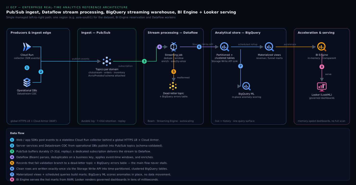
The eight numbered steps trace one event’s journey: it is produced (1), buffered durably in Pub/Sub (2), pulled by Dataflow where it is validated, de-duplicated, windowed by event time, and enriched (3) — with malformed records forked to a dead-letter branch (4) — then written exactly-once into partitioned, clustered BigQuery tables (5), rolled into materialized views and scored by BigQuery ML (6), accelerated in memory by BI Engine (7), and finally rendered in a governed Looker dashboard (8).
Component breakdown
| Component | Role in the path | Key configuration choices |
|---|---|---|
| Pub/Sub topics | Durable ingest buffer; decouples producers from consumers; absorbs spikes | Topic per event domain; attach Avro/Protobuf schema; set message retention (7→up to 31 days) for replay; enable exactly-once delivery on subscriptions; ordering keys only where strictly needed |
| Pub/Sub subscriptions | Deliver to Dataflow; isolate consumers | Dedicated subscription per consumer; dead-letter topic + max delivery attempts; tune ack deadline; separate subscription for any direct BigQuery export use cases |
| Cloud Run collector | Server-side event endpoint for web/app SDKs | Stateless, autoscaling to zero; validates and publishes to Pub/Sub; behind a global HTTPS Load Balancer + Cloud Armor |
| Datastream | Low-latency CDC from operational DBs into the stream | Streams MySQL/Postgres/Oracle changes to Pub/Sub or BigQuery; pairs with Dataflow templates for transform |
| Dataflow (Beam) streaming job | Parse, validate, dedupe, window, enrich, route, write | Streaming Engine on; horizontal autoscaling; event-time windowing + watermarks + allowed lateness; dedupe on business key; Storage Write API exactly-once to BigQuery; dead-letter branch; side inputs / Bigtable for enrichment |
| BigQuery dataset/tables | Streaming warehouse: live + historical store of record | Time-unit partitioning (DAY/HOUR) on event time; clustering on high-cardinality filters (region, channel, sku); partition expiration for raw retention; materialized views + scheduled queries for marts |
| BigQuery ML | In-warehouse scoring without data movement | Anomaly/forecast models on the conversion or volume stream; inference via ML.PREDICT in scheduled queries |
| BigQuery BI Engine | In-memory acceleration of the serving tables | Reserve memory (GiB) in the dataset region; size to the hot marts + MVs; transparent — no query change; monitor hit ratio |
| Looker (LookML) | Semantic model + governed dashboards | Define metrics/funnel once in LookML; row-level access via user attributes; persist derived tables (PDTs) for heavy rollups; dashboards with auto-refresh |
A few choices deserve the why, because they are where this architecture earns its keep.
Pub/Sub schemas and a dead-letter topic are non-negotiable, not nice-to-haves. The failure that kills naive pipelines is a single malformed event that the consumer can’t parse, retries forever, and backs up the whole subscription. Attaching a schema rejects garbage at publish time; the dead-letter topic catches whatever slips through so the main flow never stalls and you can replay or inspect failures later.
Dataflow exists specifically to do what the Pub/Sub→BigQuery direct subscription cannot. The direct subscription is genuinely useful for raw, append-only landing with no transformation. But it can’t deduplicate on a business key, can’t put a late event into the correct historical window (it lands it in “now”), can’t enrich against reference data, and can’t route bad records aside. Those four jobs are the difference between a dashboard you trust and one you don’t. Beam’s event-time windowing with watermarks and allowed lateness is the mechanism that makes “what happened in the 14:05 minute” correct even when some 14:05 events show up at 14:09.
Partitioning and clustering are the cost-control mechanism, applied at the store. A query filtered to today and one region should scan a few partitions and a few clusters, not the whole table. Get the partition key (event time) and cluster keys (the columns dashboards filter on) right and BigQuery’s bytes-scanned — what you pay for on-demand — drops by orders of magnitude. This is the layer that makes the next layer affordable.
BI Engine is what makes Looker feel instant without changing a query. BigQuery is fast but is a scan engine; interactive dashboards with hundreds of users hammering filter changes want memory-speed responses. BI Engine reserves RAM in the dataset’s region and transparently serves the hot tables from memory — Looker’s existing SQL just gets answered in tens of milliseconds. You don’t rewrite anything; you size a reservation and watch the hit ratio.
Implementation guidance
Project and dataset layout. Use a dedicated Google Cloud project for the analytics platform (or one per environment: analytics-dev, analytics-prod) under your org/folder hierarchy, with a shared VPC from the landing-zone host project. BigQuery datasets are regional — co-locate the dataset, BI Engine reservation, and Dataflow workers in the same region (for example us-central1 or europe-west1) to avoid cross-region egress and latency, and to keep BI Engine eligible.
Infrastructure as code (Terraform). Provision the whole path declaratively so it’s reproducible and reviewable:
google_pubsub_schema+google_pubsub_topicper domain, withgoogle_pubsub_subscriptioncarryingdead_letter_policyandenable_exactly_once_delivery.google_bigquery_datasetandgoogle_bigquery_tablewithtime_partitioning(field = event timestamp, typeDAY),clusteringcolumns, andrequire_partition_filter = trueso no one accidentally scans all history.google_bigquery_bi_engine_reservationsized in GiB for the dataset region.- The Dataflow job via
google_dataflow_flex_template_job(or a Cloud Build/CI step runninggcloud dataflow flex-template run) pointing at your packaged Beam pipeline, withenableStreamingEngineand autoscaling parameters. google_bigquery_data_transfer_config(scheduled queries) andgoogle_bigquery_tableof type materialized view for the marts.- Looker itself is typically the managed Looker (Google Cloud core) instance, provisioned in-console/Terraform, with the LookML project in Git; the BigQuery connection uses a dedicated service account.
Keep the Beam pipeline code in its own repo with unit tests on the transforms (Beam’s TestStream lets you assert windowing and late-data behavior deterministically) and a CI pipeline that builds the Flex Template image and updates the job.
The Dataflow pipeline, concretely. A streaming Beam pipeline (Java or Python) that: reads from the Pub/Sub subscription with message attributes for event time; applies a fixed or sliding window with an event-time watermark and allowed_lateness; deduplicates with a stateful Deduplicate/keyed dedup on the business key over a time bound; enriches via a side input refreshed periodically (catalog/segment) or a per-key lookup to Bigtable/Memorystore for high-cardinality joins; branches invalid records to a dead-letter PubsubIO/BigQuery errors table with the failure reason; and writes valid rows to BigQuery using BigQueryIO.write() with the Storage Write API at-least-once or exactly-once method. Prefer Storage Write API over legacy streaming inserts — it’s the current path, cheaper, and supports exactly-once.
Networking. The Cloud Run collector sits behind a global external HTTPS Load Balancer with Cloud Armor (WAF, geo/rate rules, bot defense) and Cloud CDN where applicable. Dataflow workers run in your shared VPC subnet with Private Google Access, so they reach Pub/Sub and BigQuery over Google’s private network with no public egress; use --no_use_public_ips. Lock data services behind VPC Service Controls perimeters so BigQuery and Pub/Sub can’t exfiltrate data outside the perimeter even with valid credentials. Looker reaches BigQuery over Google’s network; restrict Looker admin/UI access via IAP or an allowlist.
Identity and access (least privilege). Give each component its own service account: the collector SA gets pubsub.publisher on its topics only; the Dataflow worker SA gets pubsub.subscriber on its subscriptions, bigquery.dataEditor on the target dataset, and read on enrichment sources; the Looker SA gets bigquery.dataViewer + bigquery.jobUser on the serving dataset and nothing else. Humans get access through groups mapped to IAM roles, not individual grants. Use column-level access (policy tags via Data Catalog/Dataplex) to mask PII (email, payment tokens) so analysts query behavior without seeing identifiers, and authorized views / row-level access to scope what each market or team sees. Looker layers its own row-level controls on top via user attributes for defense in depth.
Enterprise considerations
Security and Zero Trust. The perimeter is identity- and context-based, not network-trust-based. No service account has standing broad access; each is scoped to exactly the topics/datasets it needs, and access is brokered through groups. VPC Service Controls create a data perimeter so even a leaked key can’t move BigQuery data out. Dataflow runs without public IPs over Private Google Access. PII is masked with column-level policy tags so most analysts never see raw identifiers; access to unmasked columns is a separate, audited grant. Cloud Armor fronts the only public ingress (the collector). Every access is logged in Cloud Audit Logs, and Pub/Sub schemas plus the dead-letter path mean malformed or hostile payloads are contained, not propagated. This is Zero Trust applied to a data platform: verify identity, grant least privilege, segment the data, and assume any single credential can be compromised.
Cost optimization. Costs split across four meters, and the architecture is shaped to keep each low:
- BigQuery query — the big one. Partition + cluster so dashboard queries scan kilobytes-to-megabytes, not terabytes; require a partition filter to prevent accidental full scans; serve dashboards from materialized views and BI Engine so repeated reads don’t re-scan raw data. Choose on-demand pricing for spiky exploration or a BigQuery editions slot reservation (with autoscaling) for predictable heavy workloads — model both against your scan volume.
- BI Engine — a fixed reservation cost; size it to the hot marts/MVs, not the whole warehouse, and watch the hit ratio to right-size.
- Dataflow — billed on worker vCPU/memory/time. Streaming Engine plus autoscaling means you pay for current load; cap
maxNumWorkersto bound spend. - Pub/Sub — billed on throughput; cheap relative to the rest, and retention is the main lever.
The decisive cost move is that dashboards never hit raw history: BI Engine + materialized views absorb the interactive load, so analyst curiosity doesn’t translate into scan bills.
Scalability. Every stage scales independently. Pub/Sub is effectively unbounded throughput and absorbs spikes as a buffer. Dataflow autoscaling adds workers as the backlog or input rate grows and removes them when it drains. BigQuery’s storage and (with editions autoscaling) compute scale without capacity planning. BI Engine scales by adding reservation memory. Because the stages are decoupled by the Pub/Sub log, a slow downstream never backs up producers — the buffer just grows and drains. The same design runs at thousands of events/sec for a mid-market company and at millions/sec for a large enterprise; only the autoscaling ceilings and reservation sizes change.
Reliability and DR (RTO/RPO). The durable Pub/Sub log is the backbone of recoverability: with retention configured, you can replay from a timestamp to rebuild a derived table after a logic bug or a bad deploy, and the dead-letter topic preserves anything that failed. Dataflow checkpoints state in Streaming Engine, so a worker failure doesn’t lose in-flight data; exactly-once writes mean a retry doesn’t double-count. For RPO: with Pub/Sub retention and replay, effective data loss approaches zero for the window you retain — design for an RPO inside your retention period (e.g., 7 days). For RTO: BigQuery is regional with high availability inside the region; for regional-outage resilience, choose a multi-region BigQuery location (US/EU) or replicate critical datasets to a second region and keep the Dataflow + Pub/Sub deploy reproducible via Terraform so you can stand the pipeline back up in a paired region in well under an hour. Most enterprises target RTO of an hour or two for the dashboard layer and minutes for ingest (Pub/Sub is global-edge resilient).
Observability. Cloud Monitoring + Logging give you the operational picture: Pub/Sub subscription backlog / oldest-unacked-message age (the leading indicator that processing is falling behind), Dataflow system lag / data freshness / watermark and worker autoscaling, BigQuery slot utilization and bytes scanned, BI Engine hit ratio, and dead-letter topic depth (should be near zero; an alert fires if it grows). Looker’s own usage analytics show slow dashboards and heavy queries. Set SLOs on end-to-end freshness (event-produced to queryable) and alert on backlog age and dead-letter growth — those two catch most real incidents early.
Governance. Dataplex / Data Catalog provide the data catalog, lineage, and policy tags that drive column masking; this is where data products are described and discovered. Looker’s LookML is the governed semantic layer — metrics and the funnel are defined once, version-controlled in Git, and access-scoped, so every team computes “conversion rate” the same way. IAM through groups, audit logs, and VPC Service Controls round out a setup that satisfies SOC 2 / ISO controls and data-residency requirements (pin region to the required jurisdiction).
Reference enterprise example
Lumen & Loom is a mid-market omnichannel home-goods retailer: roughly 900 employees, an e-commerce site and mobile app, 40 physical stores feeding point-of-sale events, and about ₹4,200 crore in annual revenue. Their merchandising and growth teams were flying blind intraday — the warehouse refreshed nightly, so promotions were planned on yesterday’s data, stockouts on hero SKUs surfaced a day late, and a payment-gateway slowdown one Black-Friday-eve cost them an estimated ₹1.1 crore in lost conversion before anyone noticed at the morning standup. They set a target: operational dashboards no more than 90 seconds behind reality, sub-second interactivity, and no per-dashboard scan bills, on a platform a five-person data team could run.
They deployed exactly this architecture in asia-south1 (Mumbai) for data residency. Volume at peak is about 35,000 events/sec across clickstream, orders, inventory, and POS. The web/app SDKs post to a Cloud Run collector behind a global HTTPS LB with Cloud Armor; server services and Datastream CDC from their Postgres order DB publish to four Pub/Sub topics, each with an attached Avro schema and a dead-letter topic. A single Dataflow streaming job (Streaming Engine, autoscaling 4→30 workers) deduplicates on event_id, applies 1-minute event-time windows with 4 minutes of allowed lateness, enriches orders with the product catalog via a refreshed side input, routes ~0.3% malformed events to a dead-letter table, and writes via the Storage Write API (exactly-once) into BigQuery tables partitioned by event-hour and clustered on (region, channel, sku).
Materialized views maintain revenue-by-minute-by-region-by-channel and the checkout funnel; a BigQuery ML anomaly model scores the conversion stream every minute. A BI Engine reservation of 40 GiB sits in front of the marts, and Looker (Google Cloud core) serves the operational dashboards with LookML-defined metrics, row-level access by region for store managers, and column masking on customer email/payment tokens.
The outcome after one quarter:
- End-to-end freshness: ~35 seconds (event produced to queryable in Looker), well inside the 90-second target.
- Dashboard p95 latency: ~280 ms with BI Engine hit ratio above 90% — interactive even with ~120 concurrent analysts and store managers.
- The payment-degradation scenario, replayed: the conversion-anomaly alert now fires within ~2 minutes of a gateway slowdown, versus a day; on-call reroutes to the backup processor before material revenue is lost.
- Cost: the whole platform runs about ₹9–11 lakh/month — Dataflow workers and the BI Engine reservation are the largest lines; BigQuery query cost stayed flat as usage grew because dashboards hit MVs + BI Engine, never raw history. They evaluated a slot reservation and stayed on on-demand because partitioning kept scan volume low.
- Operability: the five-person team runs it with two alerts that matter — Pub/Sub backlog age and dead-letter depth — and rebuilt a mart once by replaying Pub/Sub after a LookML metric bug, with zero data loss.
The decision that paid off most was resisting the temptation to point Looker straight at the Pub/Sub→BigQuery direct subscription’s raw table. Putting Dataflow in the middle (for dedup, windowing, enrichment, dead-lettering) and BI Engine at the end (for speed and cost) is the entire difference between the “works in the demo” version and the one merchandising now plans the homepage on every afternoon.
When to use it
Use this architecture when you need genuinely fresh analytics (seconds-to-minutes) over event streams, and you want the same store to answer historical questions, and you have interactive dashboard users who need fast, governed, self-serve access. It is the sweet spot for clickstream and product analytics, real-time operational/revenue monitoring, IoT and telemetry analytics, fraud/anomaly surfacing, and any “live business dashboard” use case. It scales cleanly from a small team to a large enterprise because every tier is managed and elastic.
The trade-offs and anti-patterns:
- Don’t skip Dataflow to save effort. The Pub/Sub→BigQuery direct subscription is great for raw append-only landing with no transformation, but if you need dedup, correct late-data windowing, enrichment, or dead-lettering — and real-time analytics almost always does — you need the processing tier. Pointing dashboards at an un-deduped, un-windowed raw table is the most common way this goes wrong.
- Don’t let Looker query raw history. Without materialized views and BI Engine, every filter change is a full-table scan: slow dashboards and a runaway bill. Pre-aggregate and accelerate.
- Don’t over-use ordering keys or sub-second windows. Strict Pub/Sub ordering and tiny windows add latency and cost; apply event-time ordering in Dataflow only where business logic truly needs it.
- Don’t cross regions. Co-locate Pub/Sub-adjacent processing, the BigQuery dataset, and BI Engine in one region; cross-region adds latency and egress and can disqualify BI Engine.
Alternatives, and when they fit better. If your latency tolerance is hours, not seconds, skip the streaming tier entirely and use scheduled batch loads into BigQuery — cheaper and simpler. If you need true sub-second per-record operational lookups (serving an app feature, not a dashboard) rather than analytical aggregation, pair this with Bigtable as the low-latency serving store, since BigQuery is a scan engine, not a key-value store. If your team lives in open-source streaming and wants Kafka semantics, Pub/Sub Lite or self-managed Kafka on GKE plus Dataproc/Flink is a heavier but more portable substitute for the Pub/Sub + Dataflow pair. And if you’re standardizing on Spark and the lakehouse rather than the warehouse, Dataproc + BigLake/Iceberg with Looker on top is the analogous pattern — but for a managed, serverless, warehouse-centric real-time analytics platform on Google Cloud, Pub/Sub → Dataflow → BigQuery → BI Engine → Looker is the reference to reach for first.
Going deeper
The overview is enough to draw the architecture. This section is what you need to operate it — the mechanics that decide whether the numbers in the reference example are real or aspirational. It is deliberately advanced; skim it now, return to it when you build.
Windowing, watermarks, and late data — the actual mechanics
The whole reason Dataflow sits in the middle is to make time correct. Two clocks matter. Processing time is when a worker happens to see an event; event time is when the event actually occurred (carried in a message attribute or a field in the payload). Real streams reorder: an event that occurred at 14:05:30 can arrive at a worker at 14:09 because a phone was in a tunnel. If you bucket by processing time, that sale lands in the 14:09 minute and every intraday chart is subtly wrong.
A watermark is Beam’s running estimate of “we have probably now seen all events with event time ≤ T.” It advances as data flows. A window (say, fixed 1-minute buckets) fires — emits its aggregate — when the watermark passes the window’s end. Allowed lateness keeps a fired window’s state in memory for an extra span so stragglers can still update it; triggers decide when to emit (on the watermark, and again on each late arrival); accumulation mode decides whether a re-fire replaces (accumulating) or adds to (discarding) the previous result.
import apache_beam as beam
from apache_beam.transforms.window import FixedWindows
from apache_beam.transforms.trigger import AfterWatermark, AfterProcessingTime, AccumulationMode

windowed = (
    events
    | "KeyBySku" >> beam.Map(lambda e: (e["sku"], e))
    | "Window" >> beam.WindowInto(
        FixedWindows(60),                                  # 1-minute event-time windows
        trigger=AfterWatermark(late=AfterProcessingTime(10)),  # fire on watermark, then on late arrivals
        allowed_lateness=240,                              # 4 minutes of grace
        accumulation_mode=AccumulationMode.ACCUMULATING,   # late panes supersede earlier ones
    )
)
Trace three events against a 14:05:00–14:06:00 window with 4-minute allowed lateness:
| Event occurs | Arrives | Lands in window | Effect |
|---|---|---|---|
| 14:05:30 | 14:05:45 | 14:05 | On time — counted in the first (on-watermark) firing |
| 14:05:10 | 14:09:30 | 14:05 | Late but within 4 min — re-fires the 14:05 window with an updated total |
| 14:05:50 | 14:12:00 | dropped | >4 min late — beyond allowed lateness; route to a late-data side output so it isn’t silently lost |
The BigQuery consequence of accumulating mode is that a window can emit twice — once on time, once corrected. You handle that either by keying the aggregate row on (window_start, sku, region) and writing with a MERGE/upsert, or by writing correction rows and summing in a materialized view. This is why the raw dedup key and the aggregate key both matter. Beam’s TestStream lets you unit-test exactly this behavior deterministically — assert that the third event is dropped and the second updates the pane — before it ever runs on live traffic.
“Exactly-once” is three separate guarantees, not one
Beginners read “exactly-once” once and assume the whole pipeline is safe. It is really three independent guarantees, and you need all three plus a business-key dedup:
- Pub/Sub exactly-once delivery (a subscription flag) means a message isn’t re-delivered to the same subscriber within its ack window. It does not stop a producer from publishing the same logical event twice after a client-side retry — that is a brand-new message with a new message ID.
- Dataflow exactly-once processing comes from Beam checkpointing shuffle state in Streaming Engine, so a retried bundle after a worker crash doesn’t double-count within the pipeline.
- Exactly-once writes to BigQuery come from the Storage Write API using a committed-type stream with per-append offsets: if an append is retried, the offset makes the duplicate a no-op.
None of those three catches a producer that published the order twice — that requires an explicit dedup on a business key (event_id) inside Dataflow, bounded by a time window (you can’t remember every key forever). So the honest mental model is: delivery + processing + write guarantees stop the infrastructure from duplicating; the business-key dedup stops the producer from duplicating. On the write API itself: the default stream is at-least-once, cheapest, and highest-throughput (fine when you dedup upstream); committed streams give exactly-once at a little more cost. Both are the current path and far preferable to the legacy tabledata.insertAll streaming inserts (best-effort insertId dedup, higher cost, a shrinking quota surface).
The dual store: BigQuery for questions, Bigtable for lookups
BigQuery is a scan engine. It is superb at “sum revenue by region for the last hour” and hopeless at “give me the live state of this one cart in 3 milliseconds at 50,000 QPS” — that pattern would run a query per lookup and melt your slots and your bill. When a product feature (not a dashboard) needs per-key, sub-millisecond reads at high concurrency, add a second sink: fork a write from the same Dataflow job into Bigtable, keyed by the entity.
import apache_beam as beam
from apache_beam.io.gcp.bigtableio import WriteToBigTable
from google.cloud.bigtable.row import DirectRow

def to_bt_row(agg):
    # entity-first, NOT time-first, so writes spread across tablets instead of hotspotting one
    key = f'{agg["sku"]}#{agg["region"]}'.encode()
    row = DirectRow(row_key=key)
    row.set_cell("stats", b"revenue_1m", str(agg["revenue"]).encode())
    return row

(live
 | "ToBigtableRow" >> beam.Map(to_bt_row)
 | "WriteBigtable" >> WriteToBigTable(
       project_id=PROJECT, instance_id="live-serving", table_id="live_stats"))
This is the read-model split (a CQRS flavour): one event stream, two stores shaped for two access patterns — BigQuery for analytical aggregation, Bigtable for key-value serving. The single most important Bigtable decision is the row key: a key that leads with a timestamp (or any monotonically increasing value) funnels every new write to one tablet and hotspots it, so lead with the entity (sku#region, a hashed prefix, or a reversed timestamp) to spread load. Because both stores are downstream of the durable Pub/Sub log, rebuilding Bigtable after a bug is the same move as rebuilding a BigQuery mart: replay from a timestamp and let the pipeline repopulate. Row-key design, app profiles, and single-cluster vs replicated trade-offs are the subject of the Bigtable deep dive.
What BI Engine actually accelerates (and what silently falls back)
BI Engine is transparent, which is a strength and a trap. It accelerates SELECT queries over supported tables when the query uses features BI Engine supports and the reservation has free memory. Queries that use unsupported constructs — certain functions, external/wildcard tables, some complex joins — silently fall back to ordinary BigQuery. You still get the right answer, just not the memory-speed path, and because it’s silent you may not notice your “accelerated” dashboard is quietly scanning bytes and billing for them. The tell is in INFORMATION_SCHEMA:
SELECT
  bi_engine_statistics.bi_engine_mode AS mode,   -- FULL, PARTIAL, or DISABLED
  COUNT(*) AS jobs
FROM `region-asia-south1`.INFORMATION_SCHEMA.JOBS
WHERE creation_time > TIMESTAMP_SUB(CURRENT_TIMESTAMP(), INTERVAL 1 DAY)
  AND statement_type = 'SELECT'
GROUP BY mode
ORDER BY jobs DESC;
If most Looker jobs show PARTIAL or DISABLED, either the reservation is undersized or the dashboards use unsupported SQL — rework the mart or the query, don’t just buy more memory. Size the reservation to the hot marts and materialized views (the tables Looker actually hits), not the whole warehouse, and pin them with preferred_tables so BI Engine spends its RAM where it pays off. Watch acceleration coverage as a first-class metric, not just “is BI Engine on.”
Schema evolution without breaking a 24/7 stream
Events change shape while the pipeline is running; you cannot take a real-time platform down to add a column. The safe moves are all additive. Pub/Sub schemas support revisions: add optional fields and roll producers forward while old consumers keep working. BigQuery allows additive changes online — add NULLABLE or REPEATED columns, and relax REQUIRED→NULLABLE — without rewriting the table; you then update the Storage Write API stream to the new schema so new rows carry the new field. What you must never do on a live stream is rename or retype a column in place — that breaks in-flight writes and historical queries. Instead add a new column, dual-write during a transition, backfill history with a MERGE, and retire the old column once nothing reads it. Treat the schema like an API with a compatibility contract, because to every producer and every dashboard, it is one.
Where the ~35 seconds of latency actually goes
The reference example’s ~35-second freshness is a budget, and knowing how it’s spent tells you which knob to turn. Roughly: producer batching/flush (~1–3 s depending on SDK flush interval) → Pub/Sub publish + deliver (sub-second) → Dataflow bundle + window trigger cadence + the Storage Write API commit interval (triggering_frequency, e.g. 5 s) — this stage dominates — → BigQuery queryability (a second or two after commit) → BI Engine (tens of ms). The single biggest lever is the window/trigger/commit cadence: shrink the window, trigger more often, or shorten the commit interval and freshness drops toward single-digit seconds. But every one of those costs more (more frequent commits, more worker churn) and, with accumulating windows, produces more correction panes to reconcile. That is the core latency-versus-cost trade-off of streaming analytics: freshness is bought with money and complexity, so buy exactly as much as the business decision needs — 35 seconds is plenty to reroute a payment processor; you do not need 3.
Practice challenges
Work these in order — they build the pipeline left to right, then stress the hard parts. Commands are current-surface gcloud/bq/Beam; substitute your own project, dataset, and region for the placeholders. No runtime is assumed; reason through each before revealing the solution.
1. (Beginner) Stand up the ingest layer with a schema and a dead-letter path. Create a Pub/Sub topic clickstream bound to an Avro schema, a dead-letter topic, and a subscription for Dataflow that has exactly-once delivery and dead-lettering after 5 attempts.
<details> <summary>Solution</summary>
# 1. Register the schema (clickstream.avsc holds an Avro record definition)
gcloud pubsub schemas create clickstream-schema \
  --type=avro --definition-file=clickstream.avsc

# 2. Topic bound to the schema, 7-day retention, binary Avro encoding
gcloud pubsub topics create clickstream \
  --schema=clickstream-schema --message-encoding=binary \
  --message-retention-duration=7d

# 3. Dead-letter topic
gcloud pubsub topics create clickstream-dlq

# 4. Subscription for Dataflow: exactly-once delivery + DLQ after 5 tries
gcloud pubsub subscriptions create clickstream-df \
  --topic=clickstream \
  --enable-exactly-once-delivery \
  --dead-letter-topic=clickstream-dlq \
  --max-delivery-attempts=5 \
  --ack-deadline=60
Why: the schema rejects malformed payloads at publish time and the DLQ catches the rest, so one bad event can never back up the whole subscription — the failure mode that kills naive pipelines. (Grant the Pub/Sub service account pubsub.publisher on the DLQ or dead-lettering silently no-ops.)
</details>
2. (Beginner) Create a warehouse table that is cheap to query by design. Make a BigQuery table events.orders partitioned by event hour, clustered on (region, channel, sku), that forces a partition filter on every query.
<details> <summary>Solution</summary>
CREATE TABLE analytics.events.orders (
  event_time TIMESTAMP,
  event_id   STRING,
  region     STRING,
  channel    STRING,
  sku        STRING,
  revenue    NUMERIC
)
PARTITION BY TIMESTAMP_TRUNC(event_time, HOUR)
CLUSTER BY region, channel, sku
OPTIONS (require_partition_filter = TRUE);
Equivalent CLI:
bq mk --table \
  --time_partitioning_field=event_time --time_partitioning_type=HOUR \
  --clustering_fields=region,channel,sku \
  --require_partition_filter \
  --schema=event_time:TIMESTAMP,event_id:STRING,region:STRING,channel:STRING,sku:STRING,revenue:NUMERIC \
  analytics:events.orders
Why: partitioning + clustering is the cost-control layer; require_partition_filter turns “someone forgot a WHERE clause” from a five-figure surprise into a query error.
</details>
3. (Intermediate) Prove the guardrail, then measure the savings. Write a query that BigQuery rejects against the table above, then fix it, and use a dry run to show how few bytes the corrected query scans.
<details> <summary>Solution</summary>
# Rejected: no partition filter → error, nothing runs, nothing billed
bq query --use_legacy_sql=false --dry_run \
'SELECT region, COUNT(*) FROM `analytics.events.orders` GROUP BY region'
# Error: Cannot query over table ... without a filter over column(s) 'event_time'
#        that can be used for partition elimination

# Corrected: a partition filter prunes to a few hours of data
bq query --use_legacy_sql=false --dry_run \
'SELECT region, COUNT(*) AS orders
 FROM `analytics.events.orders`
 WHERE event_time >= TIMESTAMP("2026-07-19 00:00:00 UTC")
 GROUP BY region'
# Query successfully validated. ... will process N MB   (not the whole table)
Why: --dry_run returns the bytes-that-would-be-scanned without running or billing — the fastest way to catch a query that would scan all history before it does.
</details>
4. (Intermediate) Accelerate the serving layer and confirm it’s working. Reserve 40 GiB of BI Engine in the dataset’s region, then check what fraction of dashboard queries are actually accelerated.
<details> <summary>Solution</summary>
resource "google_bigquery_bi_engine_reservation" "analytics" {
  project  = "analytics-prod"
  location = "asia-south1"
  size     = 42949672960          # 40 GiB expressed in bytes (40 * 1024^3)
}
-- Acceleration coverage over the last day
SELECT bi_engine_statistics.bi_engine_mode AS mode, COUNT(*) AS jobs
FROM `region-asia-south1`.INFORMATION_SCHEMA.JOBS
WHERE creation_time > TIMESTAMP_SUB(CURRENT_TIMESTAMP(), INTERVAL 1 DAY)
  AND statement_type = 'SELECT'
GROUP BY mode ORDER BY jobs DESC;
Why: BI Engine falls back to plain BigQuery silently when a query isn’t supported or memory runs out; bi_engine_mode (FULL/PARTIAL/DISABLED) is how you tell acceleration from an expensive illusion.
</details>
5. (Advanced) Reason about late data. Given 1-minute fixed windows, 4 minutes of allowed lateness, and accumulating mode, state which window each event lands in and what the aggregate table ultimately shows for these three events (all for sku=A): occurs 14:05:30 / arrives 14:05:45; occurs 14:05:10 / arrives 14:09:30; occurs 14:05:50 / arrives 14:12:10.
<details> <summary>Solution</summary>
| Event (occurs → arrives) | Window | What happens |
|---|---|---|
| 14:05:30 → 14:05:45 | 14:05 | On time; counted in the on-watermark firing (count = 1) |
| 14:05:10 → 14:09:30 | 14:05 | Late but ≤ 4 min; the 14:05 window re-fires with an updated total (count = 2) |
| 14:05:50 → 14:12:10 | none | > 4 min late; dropped past allowed lateness — send it to a late-data side output so it isn’t lost |
The 14:05 aggregate row is written, then superseded when the late event re-fires the pane; key the row on (window_start, sku) and upsert with MERGE so the correction replaces rather than duplicates.
Why: windows + watermarks + allowed lateness are what make “what happened in the 14:05 minute” correct even when some 14:05 events arrive minutes later; anything past the lateness bound is a deliberate, observable drop, not a silent one. </details>
6. (Advanced) Add a sub-millisecond serving path, then rebuild it from the log. Fork a per-sku/region write from Dataflow into Bigtable with a non-hotspotting row key, and describe how you’d rebuild that Bigtable table after a bug without re-ingesting from producers.
<details> <summary>Solution</summary>
import apache_beam as beam
from apache_beam.io.gcp.bigtableio import WriteToBigTable
from google.cloud.bigtable.row import DirectRow

def to_bt_row(agg):
    key = f'{agg["sku"]}#{agg["region"]}'.encode()   # entity-first → spreads across tablets
    row = DirectRow(row_key=key)
    row.set_cell("stats", b"revenue_1m", str(agg["revenue"]).encode())
    return row

(live
 | "ToBigtableRow" >> beam.Map(to_bt_row)
 | "WriteBigtable" >> WriteToBigTable(
       project_id="analytics-prod", instance_id="live-serving", table_id="live_stats"))
Rebuild by replaying the durable Pub/Sub log from a timestamp — the same subscription must retain acked messages:
gcloud pubsub subscriptions update clickstream-df --retain-acked-messages
gcloud pubsub subscriptions seek   clickstream-df --time=2026-07-19T00:00:00Z
Why: BigQuery answers aggregate questions but can’t serve per-key reads at millisecond latency — Bigtable can, and because both sinks live downstream of the Pub/Sub log, “rebuild the serving store” is just “replay the log.” A time-leading row key would hotspot one tablet; sku#region distributes writes.
</details>
Common beginner mistakes
- “The Pub/Sub→BigQuery direct subscription is the whole pipeline.” It is only raw, append-only landing. It cannot dedupe on a business key, cannot put a late event in the right window, cannot enrich, and cannot dead-letter. The right model: the direct subscription is a shortcut for un-transformed landing; anything you’d actually trust on a dashboard needs Dataflow in the middle.
- “Exactly-once delivery means my counts can’t double.” Delivery, processing, and writes are three separate guarantees, and none of them stops a producer from publishing the same order twice. The right model: infrastructure guarantees prevent infrastructure duplication; a business-key (
event_id) dedup in Dataflow prevents producer duplication. You need both. - “Late events are basically on time, so bucket by arrival.” Bucketing by processing time puts a 14:05 sale that arrives at 14:09 into the 14:09 minute and quietly corrupts every intraday chart. The right model: bucket by event time, let watermarks + allowed lateness handle stragglers, and route anything too late to a side output.
- “Point Looker at the raw events table — it’s live and simple.” Every filter change becomes a full-table scan: slow dashboards and a runaway bill. The right model: dashboards read materialized views accelerated by BI Engine; raw history is for backfills and ad-hoc investigation, not interactive clicking.
- “BI Engine is on, so everything is fast.” Unsupported SQL and memory pressure make it fall back to plain BigQuery silently. The right model: treat
bi_engine_modecoverage as a metric, size the reservation to the hot tables, and rework queries that won’t accelerate. - “Turn on Pub/Sub ordering everywhere to be safe.” Strict ordering serializes delivery and adds latency and cost you usually don’t need. The right model: order by event time inside Dataflow where business logic requires it, and reserve Pub/Sub ordering keys for the rare cases that truly need per-key sequence.
- “Streaming inserts and the Storage Write API are the same thing.” Legacy
tabledata.insertAllis best-effort, pricier, and being superseded. The right model: use the Storage Write API (default stream for at-least-once + upstream dedup, or committed stream for exactly-once) — it’s the current, cheaper path. - “BigQuery can also serve the app’s per-record lookups.” It’s a scan engine; a query-per-lookup at high QPS will exhaust slots and cost. The right model: for sub-millisecond key-value serving, fork a write to Bigtable and keep BigQuery for aggregation.
- “One region or many — doesn’t matter much.” Crossing regions adds egress and latency and can disqualify BI Engine entirely. The right model: co-locate Pub/Sub-adjacent processing, the BigQuery dataset, and the BI Engine reservation in a single region.
Glossary
- Real-time analytics — turning a continuous stream of events into queryable insight within seconds-to-minutes, rather than in a nightly batch.
- Pub/Sub — Google Cloud’s managed publish/subscribe messaging service; the durable buffer that decouples producers from consumers.
- Topic / subscription — a topic is the named channel producers publish to; a subscription is a consumer’s independent read cursor over that topic.
- Schema (Pub/Sub) — an Avro/Protobuf definition attached to a topic so malformed messages are rejected at publish time.
- Dead-letter topic (DLQ) — a side topic that receives messages a subscription couldn’t process after N attempts, so one poison message never stalls the flow.
- Exactly-once delivery — a Pub/Sub subscription mode that prevents re-delivery of the same message to the same subscriber within its ack window.
- Dataflow — Google Cloud’s managed, autoscaling runner for Apache Beam pipelines; the stream-processing tier here.
- Apache Beam — the unified programming model for batch and streaming data pipelines that Dataflow executes.
- Streaming Engine — the Dataflow feature that offloads pipeline state and shuffle to the service, enabling smooth autoscaling and checkpointing.
- Windowing — grouping events into time buckets (fixed, sliding, or session) so aggregates like “orders per minute” are well defined over an unbounded stream.
- Event time vs processing time — when an event actually occurred vs when a worker happened to see it; correct analytics bucket by event time.
- Watermark — Beam’s running estimate that all events up to time T have probably arrived; a window fires when the watermark passes its end.
- Allowed lateness — the extra grace period a window’s state is kept so late-arriving events can still update it before it’s finalized.
- Trigger / accumulation mode — a trigger decides when a window emits; accumulation mode decides whether a re-fire replaces (accumulating) or adds to (discarding) the prior result.
- Side input — a (usually small, periodically refreshed) reference dataset broadcast to a Beam transform for enrichment joins.
- Storage Write API — BigQuery’s current high-throughput streaming ingestion API, supporting at-least-once (default stream) and exactly-once (committed stream) writes.
- Streaming inserts — the legacy
tabledata.insertAllingestion path; best-effort dedup, pricier, superseded by the Storage Write API. - BigQuery — Google Cloud’s serverless analytical warehouse; here it is both the streaming sink and the historical store of record.
- Partitioning — physically splitting a table by a column (e.g., event hour) so queries scan only relevant partitions.
- Clustering — sorting data within partitions by chosen columns (e.g., region, sku) so filters on them read less data.
- require_partition_filter — a table option that rejects any query lacking a partition filter, preventing accidental full-table scans.
- Materialized view (MV) — a stored, automatically-maintained pre-aggregation that dashboards read instead of re-scanning raw events.
- BigQuery ML — running model training and inference (
ML.PREDICT) directly inside BigQuery with SQL, no data movement. - BI Engine — an in-memory acceleration layer that transparently serves hot BigQuery tables from RAM in tens of milliseconds.
- bi_engine_mode — a per-query indicator (FULL/PARTIAL/DISABLED) of how much of the query BI Engine accelerated.
- Looker / LookML — Looker is the governed BI and dashboard layer; LookML is its code that defines metrics, dimensions, and access once.
- Bigtable — Google Cloud’s low-latency, high-QPS wide-column key-value store, used here for sub-millisecond per-entity serving.
- Row key — Bigtable’s single sorted primary key; leading it with an entity (not a timestamp) spreads writes and avoids hotspotting one tablet.
- Datastream — managed Change Data Capture that streams row changes from operational databases into Pub/Sub or BigQuery.
- CDC (Change Data Capture) — capturing inserts/updates/deletes from a source database as an event stream.
- VPC Service Controls — a data-exfiltration perimeter around services like BigQuery and Pub/Sub, so even a valid credential can’t move data out.
- Policy tags (column-level access) — Data Catalog/Dataplex tags that mask sensitive columns (PII) unless a user has explicit access.
- Slots / reservation (BigQuery editions) — units of BigQuery compute; a reservation buys predictable capacity versus per-query on-demand pricing.
- Backlog / oldest-unacked-message age — the Pub/Sub metric showing how far behind consumers are; the leading indicator that processing is falling behind.
- System lag / data freshness (Dataflow) — how far pipeline processing trails real time; the streaming health metrics you alert on.
- RTO / RPO — Recovery Time Objective (how fast you restore service) and Recovery Point Objective (how much data loss is acceptable) in a disaster.
- Replay — re-reading events from the retained Pub/Sub log (via
seekto a timestamp) to rebuild a derived table or serving store after a bug.