In a nutshell
Every relational database you have met so far treats the schema as a logical convenience: pick whatever primary key reads nicely, add indexes later, and the engine figures out where to put the bytes. Cloud Spanner takes that choice away. In Spanner the primary key you pick is the physical sharding strategy — it decides which machine every row lands on. Get it right and one table scales linearly to millions of writes per second across the planet with real SQL and strong consistency. Get it wrong and the same table tops out on a single machine no matter how big your instance is.
Picture a giant library where every book is shelved in strict alphabetical order by its label, and one librarian owns each shelf. If you give every new book a label like 2026-07-19T10:00:00, ...:01, ...:02, they all belong on the same end shelf — so one librarian is buried under the entire intake while every other librarian stands idle. That is a hotspot, and it is the single most common way to wreck a Spanner deployment. The fix is to label books so they scatter across the whole alphabet (a random UUID, a bit-reversed number, or a hash prefix), so every librarian shares the load. Interleaving is the opposite trick: when a customer’s order slips always travel with the customer’s card, you tuck them right behind that card on the same shelf so one reach grabs everything.
Two more ideas make Spanner special and we will build up to them. A split is Spanner’s unit of load — a contiguous range of keys served by one leader — and Spanner slices the key space into more splits as load grows, but only if the keys give it room to slice. And TrueTime — Google’s globally-synchronised clock — is what lets Spanner guarantee external consistency: reads always see every write that finished before they started, anywhere on Earth, as if there were a single machine.
Level: Advanced (Expert track) · Time: ~30 min · You’ll need: comfort with SQL DDL (CREATE TABLE, primary keys, indexes) and a rough mental model of horizontal scale-out.
Prerequisites: if relational-on-GCP basics are new, skim the Cloud SQL deep dive for the single-node relational baseline Spanner departs from. The row-key reasoning here is a close cousin of the Bigtable deep dive — same hotspot physics, different engine — and the Firestore deep dive shows how another distributed GCP database handles indexes.
After this lesson you can:
- Choose a primary key that spreads writes instead of funnelling them into one split.
- Diagnose and kill a hotspot with a UUID, a bit-reversed sequence, or a hash/shard prefix — and explain the distribution-versus-locality trade-off each makes.
- Decide when to interleave a child table versus use a plain foreign key, and stay under the co-location size limit.
- Design covering secondary indexes with
STORINGandNULL_FILTERED, and spot indexes that hotspot on their own key. - Explain how splits, Paxos replication, TrueTime, and external consistency give Spanner its read/write scaling model.
- Confirm any of the above in production with query plans (
EXPLAIN ANALYZE) and Key Visualizer.
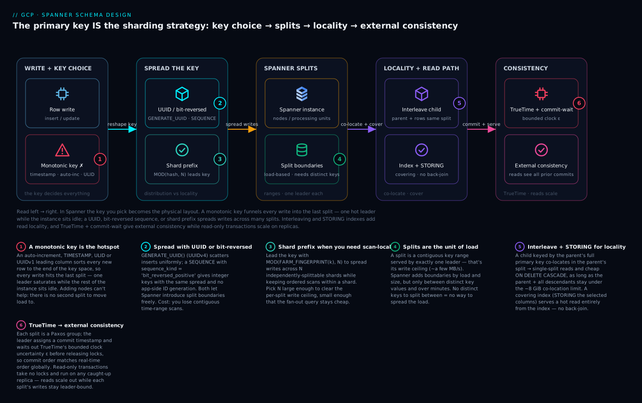
Read left → right: the key you pick (zone 1) becomes the physical layout — a monotonic key funnels every write into the last split, while a UUID, bit-reversed sequence, or shard prefix (zone 2) spreads writes across many splits (zone 3); interleaving and STORING indexes (zone 4) add read locality; and TrueTime + commit-wait (zone 5) give external consistency while read-only transactions scale on replicas.
Spanner gives you the one thing every other relational database makes you choose against: horizontal scale with external consistency and real SQL. The catch is that the schema is no longer a logical convenience — it is the physical sharding strategy. Your primary key choice decides how rows map to splits, which splits land on which servers, and therefore whether a write-heavy table tops out at a few thousand QPS or scales linearly to millions. Get the key wrong and no amount of node-adding will save you, because every write is hammering the same split.
This guide works from the storage engine up: how splits and ranges actually behave, how to choose keys that spread load, when interleaving pays off and when it traps you, how secondary indexes create their own hotspots, and how to read Key Visualizer to confirm any of it in production. Examples use GoogleSQL dialect DDL; the physical reasoning is identical for the PostgreSQL dialect.
1. Splits, nodes, and how keys map to ranges
Spanner stores rows in splits — contiguous ranges of the primary key space, sorted lexicographically by key. A split is the unit of load distribution: each split is served by a single replica leader at a time, and Spanner moves splits between servers to balance CPU and storage. A node (or its fractional equivalent, processing units, where 1000 PU = 1 node) serves many splits.
The mechanics you must internalize:
- Rows are physically ordered by primary key. Adjacent key values live in the same split until the split grows large or hot, at which point Spanner splits the range at a key boundary.
- A single split has a throughput ceiling because one leader handles its writes. The documented practical guidance is to keep a split under roughly a few MB/s of writes; beyond that you need the data spread across more splits.
- Spanner adds split boundaries based on load and size, but it can only split between distinct key values. If every write targets the same key prefix, there is no boundary to introduce — the load cannot be spread.
That last point is the whole game. A “hotspot” is not a Spanner bug; it is a schema that forces all current writes into a key range that cannot be subdivided fast enough.
Spanner can pre-split a table at load time via
gcloud spanner databases ddl updatewith split points, and it learns split boundaries over minutes as load arrives. But pre-splitting a monotonically increasing key buys you nothing, because tomorrow’s writes all land past the highest boundary anyway. The fix is always in the key shape, not in pre-splitting.
2. Choosing primary keys to avoid monotonic-key hotspots
The classic mistake is a primary key that increases (or decreases) with time: an auto-increment integer, a TIMESTAMP, a UUIDv1/ULID, or anything sequence-backed. Every new row sorts to the end of the key space, so every write hits the last split. You have built a distributed database that writes to exactly one machine.
-- ANTI-PATTERN: monotonic key. All inserts hit the highest split.
CREATE TABLE Events (
  EventId   INT64 NOT NULL,   -- from a sequence -> monotonic
  Payload   STRING(MAX),
  CreatedAt TIMESTAMP NOT NULL OPTIONS (allow_commit_timestamp = true),
) PRIMARY KEY (EventId);
Fixes, in rough order of preference:
-
Use a random UUID as the leading key column.
GENERATE_UUID()(UUIDv4) is uniformly distributed, so inserts scatter across the entire key space and Spanner can split freely.CREATE TABLE Events ( EventId STRING(36) NOT NULL DEFAULT (GENERATE_UUID()), Payload STRING(MAX), CreatedAt TIMESTAMP NOT NULL OPTIONS (allow_commit_timestamp = true), ) PRIMARY KEY (EventId); -
Swap the order of a composite key so the high-cardinality, well-distributed column leads.
PRIMARY KEY (UserId, CreatedAt)spreads writes across users;PRIMARY KEY (CreatedAt, UserId)funnels them by time. Same columns, opposite physical behavior. -
Hash a natural key into the leading column when you need a deterministic but spread key (covered in step 5).
The cost of a random key is range scans: you can no longer scan “the last hour of events” by reading a contiguous key range, because time is not the leading column. That is the central trade — distribution versus locality. Resolve it deliberately: if you query by entity (WHERE UserId = ?), lead with the entity; if you truly need time-ordered scans, accept a bit-reversed or sharded approach rather than a raw timestamp.
3. Interleaving child tables for co-located, low-latency joins
Interleaving physically co-locates a child table’s rows with their parent row, in the same split, ordered by the shared key prefix. Orders and OrderLines for the same OrderId sit next to each other on disk. The payoff:
- A parent + children read is served from one split — no cross-split fan-out, no distributed read.
ON DELETE CASCADEbecomes a cheap local operation.- Joins on the interleaving key are local; Spanner does not shuffle.
CREATE TABLE Customers (
  CustomerId STRING(36) NOT NULL DEFAULT (GENERATE_UUID()),
  Name       STRING(256),
) PRIMARY KEY (CustomerId);

CREATE TABLE Orders (
  CustomerId STRING(36) NOT NULL,
  OrderId    STRING(36) NOT NULL DEFAULT (GENERATE_UUID()),
  Total      NUMERIC,
  PlacedAt   TIMESTAMP NOT NULL OPTIONS (allow_commit_timestamp = true),
) PRIMARY KEY (CustomerId, OrderId),
  INTERLEAVE IN PARENT Customers ON DELETE CASCADE;

CREATE TABLE OrderLines (
  CustomerId STRING(36) NOT NULL,
  OrderId    STRING(36) NOT NULL,
  LineNo     INT64 NOT NULL,
  Sku        STRING(64),
  Qty        INT64,
) PRIMARY KEY (CustomerId, OrderId, LineNo),
  INTERLEAVE IN PARENT Orders ON DELETE CASCADE;
The child’s primary key must be prefixed by the parent’s full primary key — that prefix is what guarantees co-location. The trap is the interleaving (co-location) row size limit: a parent row plus all of its interleaved descendant rows must stay under ~8 GiB. A single customer with a runaway number of orders and lines will blow that ceiling and you cannot split that hierarchy across machines. Interleave one-to-few relationships (a customer’s orders, an order’s lines), never one-to-unbounded fan-outs (every event for an account that lives forever).
Decision rule: interleave when the child is small per parent and you almost always read them together. Keep tables independent when the child set is unbounded, when children are queried without the parent, or when the parent’s hierarchy could approach the size limit. A normal foreign key (step 6) gives referential integrity without forcing co-location.
4. Secondary indexes: STORING, index hotspots, and null filtering
A secondary index in Spanner is a separate, sorted table keyed by the indexed columns (with the base table’s primary key appended to make each index entry unique). That has three consequences experts plan for.
Index keys hotspot exactly like table keys. An index on a monotonic column funnels all index writes into one split, even if the base table is perfectly distributed. An index on CreatedAt recreates the timestamp hotspot in the index.
-- Same monotonic-write problem, now in the index.
CREATE INDEX OrdersByPlacedAt ON Orders (PlacedAt);
Use STORING to make an index covering. Without it, a query that selects columns not in the index does an extra back-join to the base table (one lookup per row). STORING copies those columns into the index so the query is served entirely from the index — at the cost of extra storage and write amplification.
CREATE INDEX OrdersByCustomerStatus
  ON Orders (CustomerId, Status)
  STORING (Total, PlacedAt);
-- SELECT Total, PlacedAt WHERE CustomerId=? AND Status=? is index-only.
NULL_FILTERED indexes skip rows where an indexed column is null, which shrinks sparse indexes dramatically and is the right default for “flag” columns where only a few rows qualify (e.g., an index over open tickets only).
CREATE NULL_FILTERED INDEX OrdersAwaitingFulfilment
  ON Orders (FulfilmentDueAt)
  STORING (Total) WHERE FulfilmentDueAt IS NOT NULL;
You can also interleave an index in a table (... INTERLEAVE IN <ParentTable>) so index entries co-locate with the parent, which keeps per-entity index lookups local. Use it when the index is always queried within one parent.
5. Bit-reversed sequences and key hashing for high-write tables
Sometimes you genuinely need a numeric, mostly-ordered key (foreign-key friendliness, integer joins, smaller storage than a UUID) but cannot accept the monotonic hotspot. Spanner ships a purpose-built tool: the bit-reversed positive sequence. It generates unique positive integers whose bit-reversed values are what get stored, so consecutive logical values land in completely different parts of the key space.
CREATE SEQUENCE EventSeq OPTIONS (sequence_kind = 'bit_reversed_positive');

CREATE TABLE Events (
  EventId   INT64 NOT NULL DEFAULT
              (GET_NEXT_SEQUENCE_VALUE(SEQUENCE EventSeq)),
  Payload   STRING(MAX),
  CreatedAt TIMESTAMP NOT NULL OPTIONS (allow_commit_timestamp = true),
) PRIMARY KEY (EventId);
This gives you integer keys with UUID-like write distribution and no application-side ID generation. It is the recommended replacement for auto-increment on a hot table.
The manual alternative is explicit key hashing / sharding: prepend a computed shard column derived from a hash of the rest of the key, modulo N.
CREATE TABLE EventsSharded (
  ShardId   INT64 NOT NULL,   -- MOD(FARM_FINGERPRINT(NaturalKey), 32) at write time
  NaturalKey STRING(128) NOT NULL,
  Payload   STRING(MAX),
) PRIMARY KEY (ShardId, NaturalKey);
With ShardId leading, writes spread across N=32 logical shards, each free to split independently. The cost: a query for all rows matching a NaturalKey range must fan out across all 32 shards (WHERE ShardId BETWEEN 0 AND 31 AND ...). Pick N small enough that the fan-out is cheap but large enough to clear your write ceiling — for most workloads a low double-digit number is plenty, not hundreds. Bit-reversed sequences are usually cleaner; reach for manual sharding only when you need scan locality within a shard.
6. Foreign keys, check constraints, and generated columns
Beyond keys and indexes, three schema features encode invariants so the application cannot violate them.
Foreign keys enforce referential integrity without the co-location of interleaving. Use them when you want the guarantee but the relationship is not a tight parent/child you always read together.
ALTER TABLE Orders ADD CONSTRAINT FK_Orders_Customer
  FOREIGN KEY (CustomerId) REFERENCES Customers (CustomerId);
Spanner auto-creates a backing index on the referencing columns if a usable one does not already exist; enforcement adds a read on every insert/update of the child, so foreign keys are not free on the write path.
Check constraints validate column values at write time:
ALTER TABLE Orders ADD CONSTRAINT CK_Orders_Total
  CHECK (Total >= 0);
Generated columns compute a value from other columns in the same row, and — critically — a STORED generated column can be indexed. This is the clean way to make a derived value (a normalized email, a hash shard, a status bucket) queryable without trusting the application to keep it in sync.
ALTER TABLE Customers ADD COLUMN
  EmailLower STRING(256) AS (LOWER(Email)) STORED;

CREATE INDEX CustomersByEmailLower ON Customers (EmailLower);
This pattern — a STORED generated shard column plus a leading position in the key or an index — is how you bolt hash-sharding onto an existing table without rewriting application writes.
7. Reading query plans and using Key Visualizer to find hot splits
Schema reasoning is a hypothesis; the query plan and Key Visualizer are how you confirm it.
Query plans. Use EXPLAIN / EXPLAIN ANALYZE (or the console’s plan view) and look for the failure signatures:
-
A full table scan where you expected an index seek means the index is missing, not covering, or the optimizer rejected it. Force it to validate with a hint and decide whether the forced plan is actually better:
SELECT Total, PlacedAt FROM Orders@{FORCE_INDEX=OrdersByCustomerStatus} WHERE CustomerId = @cid AND Status = @status; -
A back-join to the base table after an index seek means you are missing a
STORINGcolumn. Add it if the query is hot. -
Distributed union over many splits for a point-style query suggests your key or shard fan-out is wider than the access pattern needs.
Key Visualizer is the heatmap that proves hotspots in production. It plots key ranges on the vertical axis against time on the horizontal axis, with brightness = activity. Bright horizontal stripes that persist are the tell: a narrow key range absorbing disproportionate load — the visual signature of a monotonic key or a hot index.
# Open Key Visualizer for a database (console deep-link form).
gcloud spanner databases describe orders-db --instance=prod-instance
# Then: Console -> Spanner -> <instance> -> <database> -> Key Visualizer.
Read it like this: a single bright band fixed at the top of the key range over time is classic append-hotspot (monotonic key writing to the highest split). Diagonal bright bands indicate scans walking the key space. A healthy high-write table looks like uniform low-level noise across the whole key range — load spread everywhere, no persistent stripe.
8. Schema change rollouts and backfilling indexes safely
Spanner applies schema changes online — no downtime, no table lock — but large changes run a background process you must operate carefully.
- Adding an index backfills it. For a large table this is a long-running operation that consumes CPU and can compete with serving traffic. Create indexes during lower-traffic windows and watch instance CPU.
- Schema updates are versioned and applied as a sequence. Spanner validates each statement; an invalid one (e.g., a
NOT NULLadd on a column with existing nulls, or aCHECKthat existing rows violate) is rejected up front rather than half-applied. CREATE INDEXis non-blocking but not instant. Track it as a long-running operation and only rely on the index once it reports complete.
# Apply DDL; for big indexes prefer one statement per call so you can track each.
gcloud spanner databases ddl update orders-db \
  --instance=prod-instance \
  --ddl='CREATE INDEX OrdersByCustomerStatus ON Orders (CustomerId, Status) STORING (Total, PlacedAt)'

# List in-flight schema/backfill operations and watch progress.
gcloud spanner operations list \
  --instance=prod-instance \
  --database=orders-db \
  --type=DATABASE_UPDATE_DDL

gcloud spanner operations describe <OPERATION_ID> \
  --instance=prod-instance \
  --database=orders-db
For schema changes that cannot be expressed as a single safe DDL (changing a primary key, splitting one table into two, re-sharding), there is no in-place mutation — primary keys are immutable. You create a new table with the corrected key, dual-write or backfill via Dataflow, cut reads over, then drop the old table.
Enterprise scenario
A fintech platform team ran a ledger-style Transactions table keyed on PRIMARY KEY (TxnId), where TxnId was a ULID — time-ordered by design, so reconciliation jobs could scan “today’s transactions” as a contiguous range. It worked beautifully in staging. In production, as ingestion crossed ~12k writes/sec at month-end settlement, p99 commit latency spiked from 15 ms to over 400 ms and throughput flatlined no matter how many nodes they added.
Key Visualizer told the whole story in one screenshot: a single bright horizontal band pinned to the top of the key range, persistent across the entire window. Because ULIDs are monotonic, every insert landed in the highest split — one leader was absorbing all 12k writes/sec while the rest of a 10-node instance sat idle. Adding nodes did nothing because there was no second split to move load to.
The constraint was real: they could not abandon time-ordered reconciliation scans, and TxnId was a foreign key referenced across three other tables and external systems, so they could not simply randomize it. The fix kept TxnId as a stable business identifier but changed the physical key to a two-part shard-then-ULID design, with reconciliation rewritten to a bounded fan-out across the small shard set.
CREATE TABLE Transactions (
  ShardId INT64 NOT NULL,            -- MOD(FARM_FINGERPRINT(TxnId), 16) at write
  TxnId   STRING(26) NOT NULL,       -- ULID, still the business key
  Amount  NUMERIC NOT NULL,
  BookedAt TIMESTAMP NOT NULL OPTIONS (allow_commit_timestamp = true),
) PRIMARY KEY (ShardId, TxnId);

-- Reconciliation scans 16 shards in parallel instead of one hot tail.
-- WHERE ShardId BETWEEN 0 AND 15 AND TxnId >= @day_start AND TxnId < @day_end
With 16 shards leading the key, writes spread across 16 independently-splittable ranges. Commit p99 dropped back under 20 ms, the 10 nodes finally shared load evenly, and the band in Key Visualizer dissolved into uniform noise. Reconciliation cost 16 small range scans instead of one — negligible at their volume. The lesson the team wrote into their schema review checklist: a monotonic key is a single-machine bottleneck wearing a distributed database’s clothes, and it will pass every test that does not push real concurrent write volume.
Verify
Confirm the schema behaves before declaring victory.
-
Inspect the live schema and indexes from the information schema:
SELECT table_name, column_name, ordinal_position, is_nullable FROM information_schema.columns WHERE table_schema = '' ORDER BY table_name, ordinal_position; SELECT index_name, table_name, is_unique, is_null_filtered, index_state FROM information_schema.indexes WHERE table_schema = ''; -
Confirm an index is used for your hot query with
EXPLAIN ANALYZE— verify an index scan/seek, no full table scan, and no surprise back-join. -
Load-test at production concurrency, not staging volume. Drive concurrent writers at your real peak QPS and watch commit latency stay flat as you scale writers.
-
Read Key Visualizer during the load test. Healthy = uniform low-level activity across the key range. Failing = a persistent bright stripe.
-
Watch instance CPU during index backfills via Cloud Monitoring (
spanner.googleapis.com/instance/cpu/utilization) and confirm serving traffic is not starved.
Going deeper
Everything above is about where the bytes land. This section is about why Spanner can promise strong consistency while spreading those bytes across the planet — the machinery an experienced engineer needs to reason about latency, failover, and the read/write scaling model. None of it changes the schema rules; it explains the forces behind them.
Splits are Paxos groups, not just ranges
A split is not merely a key range — it is a Paxos replication group. Each split’s data is stored on several replicas in different failure domains: a regional instance keeps three read-write replicas across three zones of one region; a multi-region configuration (for example nam3, eur3) spreads replicas across regions and adds witness replicas that vote but hold no full data, plus optional read-only replicas that serve reads but never lead.
Within each split, exactly one replica is the leader. A write is not “done” when the leader has it — it is done when a majority quorum of the voting replicas has durably logged it via Paxos. That quorum is why Spanner survives a zone (or, in multi-region, a region) failure with zero data loss: the surviving majority already had every committed write, and Paxos simply elects a new leader from among them. It is also why a single split has a write ceiling: every write for that range funnels through one leader and one round of quorum replication. Add more distinct keys → more splits → more leaders sharing the write load. That is the entire physical argument for avoiding monotonic keys, restated at the replication layer.
TrueTime and external consistency
Spanner’s headline guarantee is external consistency (the strongest form of consistency — a global, real-time-ordered version of serializability): if transaction T1 commits before transaction T2 starts in real wall-clock time, then T1’s commit timestamp is strictly less than T2’s, even if the two ran on different machines in different continents. Reads therefore always reflect every write that finished before the read began. No stale reads, no reordering, no “eventually”.
The trick that makes this possible without a global lock is TrueTime. Ordinary distributed clocks disagree by unknown amounts, so you can never trust one machine’s timestamp against another’s. TrueTime instead exposes the clock as an interval with a bounded uncertainty ε (epsilon) — physically anchored by GPS receivers and atomic clocks in every datacenter. TT.now() returns [earliest, latest], and Google guarantees the true time lies inside that window (ε is typically a few milliseconds).
Spanner turns that bound into ordering with commit-wait. When a read-write transaction commits, the leader:
- picks a commit timestamp
s = TT.now().latest(the top of the current uncertainty window); - runs Paxos to replicate the write to a quorum;
- waits until
TT.now().earliest > s— i.e., it deliberately waits out the uncertainty ε — before releasing locks and acknowledging the client.
That short wait is the price of external consistency: by the time anyone can observe the commit, real time has provably passed s, so any later transaction is guaranteed a larger timestamp. A tighter ε (better clocks) means a shorter commit-wait, which is why Google invests in the clock hardware. The practical takeaway: a few milliseconds of commit-wait is baked into every write, so Spanner favours fewer, batched transactions over chatty per-row commits.
Read-write vs read-only transactions — the actual scaling model
Reads and writes scale by completely different rules, and knowing which you are issuing is half of Spanner performance tuning.
| Property | Read-write transaction | Read-only transaction |
|---|---|---|
| Locks | Pessimistic (two-phase locking) | None — lock-free |
| Where it runs | Leader replica(s) | Any replica caught up to the read timestamp |
| Multi-split cost | Two-phase commit across split leaders | Parallel reads, no commit |
| Commit-wait | Yes (a few ms) | None |
| Scales with | Number of splits / leaders (write ceiling per split) | Number of replicas / read-only replicas |
A read-write transaction takes locks, buffers its writes, and — if it touches more than one split — runs a two-phase commit across those split leaders, then pays commit-wait. More splits touched = more expensive the commit. This is the other reason interleaving matters: writing a parent and its children in one interleaved hierarchy is a single-split commit, whereas the same data spread across unrelated tables can turn one logical write into a distributed 2PC.
A read-only transaction takes no locks at all. Spanner assigns it a read timestamp and any replica that has applied writes up to that timestamp can serve it. That is how reads scale out independently of the write ceiling — you add read-only replicas (or nodes) and read throughput grows even though each split still has exactly one write leader.
The lever most teams under-use is staleness. A strong read must see everything committed as of “now”, so it may need a round-trip to the leader to confirm it is current. A bounded-staleness read (say, “at most 10 seconds old”) lets Spanner serve from the nearest caught-up replica with no leader round-trip — often a dramatic latency win for read-heavy or cross-region workloads that can tolerate slightly old data (dashboards, catalogues, recommendation reads). Choosing bounded staleness where correctness allows is a first-class scaling decision, not an afterthought.
Load-based splitting, sizing, and autoscaling
Spanner does not split only on size — it also does load-based splitting, watching a split’s CPU and carving a busy range even when it is small. But two constraints from the schema still bind it: it can only introduce a boundary between distinct key values, and it reacts over minutes, not milliseconds. A sudden monotonic burst outruns the splitter every time; a well-distributed key gives it room to work ahead of the load.
On sizing: 1 node = 1000 processing units, and you can provision sub-node granularity (100 PU steps) for small workloads. Each node carries a bounded amount of storage (raised over the product’s life to the order of several TB per node) and a recommended CPU target — Google advises keeping high-priority CPU under roughly 65% for regional instances and 45% per replica for multi-region, leaving headroom for failover and splitting. Managed autoscaling (GA) adjusts capacity to a target utilization, but it cannot rescue a hotspot: autoscaling adds nodes, and nodes do nothing for a single overloaded split. Fix the key first; scale second.
Choosing an instance configuration
The regional-versus-multi-region choice is a consistency-latency-cost triangle. A regional config keeps all voting replicas in one region: lowest write latency (quorum is local), survives a zone loss, but not a region loss. A multi-region config places replicas across regions with a designated leader region: it survives a full region outage and can serve strong reads closer to users, but every write pays cross-region quorum latency (commit-wait plus WAN round-trips to a distant replica). External consistency holds in both — the difference is purely how far the quorum and the leader are from your writers. Design the key for distribution first; the config decides how much each committed write costs in milliseconds.
Checklist
Practice challenges
Work these top to bottom — they escalate from spotting a hotspot to designing a full high-write ledger. Try each before opening the solution.
Challenge 1 — Spot the hotspot (beginner)
You inherit this table on a busy events pipeline. Explain in one sentence why it will not scale, and rewrite the DDL so writes spread.
CREATE TABLE PageViews (
  ViewedAt TIMESTAMP NOT NULL OPTIONS (allow_commit_timestamp = true),
  Url      STRING(2048),
) PRIMARY KEY (ViewedAt);
<details> <summary>Solution</summary>
ViewedAt is monotonic, so every insert sorts to the end of the key space and lands on the single highest split — one leader absorbs all writes. Give it a well-distributed leading key:
CREATE TABLE PageViews (
  ViewId   STRING(36) NOT NULL DEFAULT (GENERATE_UUID()),
  ViewedAt TIMESTAMP NOT NULL OPTIONS (allow_commit_timestamp = true),
  Url      STRING(2048),
) PRIMARY KEY (ViewId);
Why: a random UUID leading column scatters inserts uniformly across the key space, so Spanner can introduce split boundaries and share writes across many leaders. </details>
Challenge 2 — Kill an auto-increment without leaving integers (beginner–intermediate)
A Users table currently uses an application sequence for its UserId INT64 key and is hotspotting. The team wants to keep integer keys (smaller storage, integer joins) but stop the hotspot without generating IDs in the app. Write the DDL.
<details> <summary>Solution</summary>
CREATE SEQUENCE UserSeq OPTIONS (sequence_kind = 'bit_reversed_positive');

CREATE TABLE Users (
  UserId INT64 NOT NULL DEFAULT
           (GET_NEXT_SEQUENCE_VALUE(SEQUENCE UserSeq)),
  Email  STRING(320),
) PRIMARY KEY (UserId);
Why: a bit_reversed_positive sequence yields unique positive integers whose stored (bit-reversed) form scatters across the key space — integer keys with UUID-like write distribution and no app-side ID generation.
</details>
Challenge 3 — Interleave correctly (intermediate)
Given Customers(CustomerId) as parent, write the DDL for an interleaved Orders child so that a customer plus all their orders is a single-split read and deleting a customer removes their orders. Then state the one physical limit that decides whether interleaving is safe here.
<details> <summary>Solution</summary>
CREATE TABLE Orders (
  CustomerId STRING(36) NOT NULL,
  OrderId    STRING(36) NOT NULL DEFAULT (GENERATE_UUID()),
  Total      NUMERIC,
) PRIMARY KEY (CustomerId, OrderId),
  INTERLEAVE IN PARENT Customers ON DELETE CASCADE;
The child’s primary key must be prefixed by the parent’s full primary key (CustomerId first) — that prefix is what co-locates the rows. The limit: a parent row plus all its interleaved descendants must stay under ~8 GiB, because that hierarchy cannot be split across machines. Safe for a customer’s orders; unsafe if one customer could accumulate unbounded orders forever.
Why: co-location buys single-split reads and cheap cascade delete, but only for bounded one-to-few relationships that fit inside a split. </details>
Challenge 4 — Make a hot query index-only (intermediate)
This query is your busiest read and its plan shows an index seek followed by a back-join to the base table:
SELECT Total, PlacedAt FROM Orders
WHERE CustomerId = @cid AND Status = @status;
Write an index that serves it entirely from the index, and show how you would force the optimizer to use it while validating.
<details> <summary>Solution</summary>
CREATE INDEX OrdersByCustomerStatus
  ON Orders (CustomerId, Status)
  STORING (Total, PlacedAt);
SELECT Total, PlacedAt
FROM Orders@{FORCE_INDEX=OrdersByCustomerStatus}
WHERE CustomerId = @cid AND Status = @status;
Why: STORING (Total, PlacedAt) copies the selected columns into the index so there is no back-join — the query is covered — and the FORCE_INDEX hint lets you confirm with EXPLAIN ANALYZE that the covered plan is chosen and cheaper.
</details>
Challenge 5 — A skewed flag column (advanced)
An Orders table has a FulfilmentDueAt column that is non-null for only ~2% of rows (the ones awaiting fulfilment) and null for the rest. You need a fast “what is due, oldest first” query. A plain index on FulfilmentDueAt both bloats storage and risks a hotspot. Design a better index, and note the second-order risk you must still check.
<details> <summary>Solution</summary>
CREATE NULL_FILTERED INDEX OrdersAwaitingFulfilment
  ON Orders (FulfilmentDueAt)
  STORING (Total) WHERE FulfilmentDueAt IS NOT NULL;
Why: NULL_FILTERED indexes omit rows where the indexed column is null, so this index holds only the ~2% of rows that qualify — far smaller and cheaper to maintain. The second-order risk: FulfilmentDueAt is a timestamp, so even this sparse index is ordered by time and its tail can hotspot if due-dates cluster; if writes to it get hot, lead it with a small shard column (ShardId, FulfilmentDueAt) and fan the query out.
</details>
Challenge 6 — Design a high-write ledger with range scans (advanced)
Design the primary key for a Payments ledger that must sustain ~50k writes/sec, keep PaymentId (a ULID) as the business identifier referenced by other tables, and still support a daily reconciliation scan of “all payments for a given day”. Give the DDL, the reconciliation predicate, and justify your shard count.
<details> <summary>Solution</summary>
CREATE TABLE Payments (
  ShardId   INT64 NOT NULL,        -- MOD(ABS(FARM_FINGERPRINT(PaymentId)), 32) at write
  PaymentId STRING(26) NOT NULL,   -- ULID, still the business key
  Amount    NUMERIC NOT NULL,
  BookedAt  TIMESTAMP NOT NULL OPTIONS (allow_commit_timestamp = true),
) PRIMARY KEY (ShardId, PaymentId);

-- Reconciliation fans out across the shard set, still time-ordered within each shard:
-- WHERE ShardId BETWEEN 0 AND 31
--   AND PaymentId >= @day_start_ulid AND PaymentId < @day_end_ulid
Shard count: a single split tops out around a few MB/s (roughly a few thousand writes/sec for small rows), so ~50k writes/sec needs on the order of a dozen-plus independently-splittable shards; 32 gives comfortable headroom while keeping the reconciliation fan-out to 32 cheap range scans (not hundreds). Use ABS(...) so MOD cannot return a negative shard.
Why: leading the key with a hash shard spreads the 50k writes/sec across 32 ranges that each split independently, while the ULID second position preserves time-ordered scans within each shard — you trade one hot tail for a bounded, parallel fan-out, exactly the fintech pattern from the enterprise scenario. </details>
Common beginner mistakes
-
“Just add more nodes / turn on autoscaling to fix the hotspot.” Nodes and autoscaling add serving capacity, but a hotspot is all load funnelling into one split served by one leader. There is no second split to move that load to, so the extra nodes sit idle. Right model: fix the key shape so the load spreads across many splits; scale capacity only after that.
-
“ULID/UUIDv1 is random-looking, so it’s a safe key.” ULIDs and UUIDv1 are time-ordered by design — their leading bits encode a timestamp, so they are monotonic and hotspot exactly like an auto-increment. Use
GENERATE_UUID()(UUIDv4, genuinely random) or a bit-reversed sequence when you want spread. -
“My base table is well-distributed, so my indexes are fine.” A secondary index is a separate sorted table with its own key order. An index leading on
CreatedAtrecreates the timestamp hotspot in the index even if the base table is perfectly spread. Check every index for its own monotonic-key problem. -
“Interleave everything — co-location is always faster.” Interleaving is only safe for bounded one-to-few relationships you read together, and the parent-plus-descendants hierarchy must fit under the ~8 GiB co-location limit. Interleaving an unbounded child (every event for an account, forever) builds a hierarchy that cannot be split — a guaranteed future outage. Use a plain foreign key when the child set is unbounded or queried on its own.
-
“A timestamp primary key is fine because I need to scan by time.” That is the exact shape that funnels every write into the last split. You can have time-ordered scans without the hotspot — lead with the entity (
UserId, CreatedAt) or a shard (ShardId, CreatedAt) and accept a bounded fan-out. Distribution and locality are a deliberate trade, not a free lunch. -
“Spanner is just MySQL/Postgres that scales — my existing schema will port straight over.” In a single-node database the primary key is a logical convenience; in Spanner it is the physical sharding strategy. A schema that was perfect on Cloud SQL can hotspot instantly on Spanner. Re-derive keys from access patterns and write distribution, not from the old schema.
-
“Strong reads are the only correct choice, so all reads hit the leader.” Read-only transactions are lock-free and, with bounded staleness, can serve from the nearest caught-up replica with no leader round-trip. Insisting on strong reads for data that tolerates a few seconds of staleness throws away Spanner’s biggest read-latency lever.
Glossary
- Split — a contiguous range of the primary-key space and Spanner’s unit of load distribution; each split is served by one leader replica at a time.
- Split boundary — the key value at which Spanner divides one split into two; Spanner can only place a boundary between distinct key values.
- Leader replica — the single replica of a split that handles writes and strong reads; failover elects a new leader from the surviving quorum.
- Node / processing unit (PU) — Spanner’s capacity unit; 1 node = 1000 PU, and one node serves many splits. Not the same as a split.
- Hotspot — a key range absorbing disproportionate load because writes concentrate into a split that cannot be subdivided fast enough.
- Monotonic key — a key that always increases (or decreases): auto-increment,
TIMESTAMP, ULID, UUIDv1. Every new row sorts to the same end split — the classic hotspot. - Primary key — in Spanner, the row’s identity and its physical location; it determines which split (and therefore which server) the row lives on.
- Interleaving (co-location) — physically storing a child table’s rows inside the parent’s split, ordered by the shared key prefix, so parent + children read from one split.
- Co-location size limit — the ~8 GiB ceiling on a parent row plus all its interleaved descendants; that hierarchy cannot be split across machines.
- Secondary index — a separate, sorted table keyed by the indexed columns (with the base primary key appended); it has its own key order and can hotspot on its own.
STORING/ covering index — an index that copies extra columns so a query is served entirely from the index, avoiding a back-join to the base table.NULL_FILTEREDindex — an index that omits rows where an indexed column is null, shrinking sparse “flag” indexes dramatically.- Bit-reversed sequence — a
bit_reversed_positivesequence whose stored (bit-reversed) values scatter across the key space: integer keys with UUID-like write spread. - Shard / hash prefix — a computed leading key column (e.g.,
MOD(FARM_FINGERPRINT(k), N)) that spreads writes across N ranges while keeping scans local within a shard. GENERATE_UUID()— Spanner’s UUIDv4 generator; uniformly random, so it makes an ideal well-distributed leading key.- Foreign key — referential-integrity constraint that does not co-locate data (unlike interleaving); enforcement adds a read on the child’s write path.
- Generated column (
STORED) — a column computed from others in the same row; aSTOREDone can be indexed, the clean way to make a derived value (shard, lowercased email) queryable. - TrueTime — Google’s globally-synchronised clock exposed as an interval
[earliest, latest]with a bounded uncertainty ε, anchored by GPS and atomic clocks. - Commit-wait — the brief pause a leader takes to wait out TrueTime’s uncertainty ε before acknowledging a commit, which is what enforces external consistency.
- External consistency — Spanner’s strongest guarantee: if T1 commits before T2 starts in real time, T1’s timestamp is smaller — a global, real-time-ordered serializability.
- Read-write transaction — a locking (two-phase locking) transaction that commits via Paxos plus commit-wait, and uses two-phase commit when it spans multiple splits.
- Read-only transaction — a lock-free transaction assigned a read timestamp; any caught-up replica can serve it, so reads scale with replicas.
- Bounded staleness — a read option allowing data up to N seconds old so Spanner can serve from the nearest replica without a leader round-trip — a major read-latency lever.
- Paxos / quorum — the consensus protocol replicating each split; a write commits once a majority of voting replicas have durably logged it, which is what survives a zone/region failure.
- Key Visualizer — a Spanner heatmap of key range (vertical) versus time (horizontal) with brightness = activity; persistent bright stripes reveal hotspots.
- GoogleSQL dialect — Spanner’s native SQL/DDL dialect (used in this guide); the PostgreSQL dialect exposes the same physical engine with Postgres syntax.
EXPLAIN ANALYZE/ back-join — the query-plan tool; a “back-join” is the extra base-table lookup after an index seek that aSTORINGcolumn removes.