The first time you model Amazon DynamoDB like the relational database you already know, it works — for about a sprint. You create a Users table, an Orders table, an OrderItems table, one per entity, exactly as you would in PostgreSQL. Then the product manager asks for “all pending orders for a customer, newest first,” and you discover DynamoDB has no JOIN, no GROUP BY, and that the only way to answer your new question is a Scan that reads every item in the table and throws most of them away. The bill climbs, the p99 latency grows a shelf, and someone says the words every architect dreads: “maybe DynamoDB was the wrong choice.”
DynamoDB was not the wrong choice. The relational modeling method was. In a SQL database you normalize first — split data into tidy, non-redundant tables — and figure out the queries later, because the query planner will join whatever you ask for at read time. DynamoDB has no query planner and no joins; it trades that flexibility for guaranteed single-digit-millisecond latency at any scale. So you invert the process: you list the access patterns first, then design the schema to serve them — often collapsing every entity into one table whose partition and sort keys are generic, overloaded strings. This is single-table design, and it is the single highest-leverage skill in DynamoDB.
This article teaches that method end to end. You will learn the mental-model swap, then every technique that makes one table serve a dozen access patterns: overloaded keys, item collections, composite sort keys for hierarchies, GSI overloading, inverted and sparse indexes, the adjacency-list pattern for graphs, write sharding to defuse a hot partition, denormalization and stream-maintained aggregations, and transactions. You will model a complete e-commerce/SaaS workload into one table plus two GSIs — with the exact item shapes and every query — build it in a copy-pasteable aws CLI + Terraform lab, and, just as importantly, learn the cases where single-table design is the wrong answer and a boring multi-table or analytics design wins.
What problem this solves
The pain is not that DynamoDB is slow — it is that DynamoDB is fast only along the axes you designed for, and unforgiving everywhere else. Model it wrong and every symptom below shows up in production, usually under load, usually on a launch day.
| Symptom in production | Root cause (a modeling decision) | What single-table design does instead |
|---|---|---|
A new feature needs a Scan of the whole table |
You modeled entities, not access patterns; the query axis does not exist | Every listed pattern maps to one Query on a key or index — no Scan on the hot path |
| Reading an order needs 4 round trips (order, items, customer, shipping) | Entities live in separate tables; you are hand-rolling joins in application code | An item collection returns a parent and all its children in one Query |
| Latency is fine at 100 users, throttles at 100k | A low-cardinality partition key concentrates traffic on one partition | Overloaded keys spread load; write sharding defuses genuinely hot keys |
| The bill triples when you add “search by status” | A FilterExpression still reads (and bills) every item before discarding non-matches |
A sparse GSI indexes only the matching subset — you read what you return |
| Cross-region reads are slow for global users | Single-region table | Global tables replicate; but the keys must already be access-pattern-shaped |
| A “simple” report locks up the table | You ran analytics (aggregations, ad-hoc joins) against the OLTP table | You route analytics to S3 + Athena/Redshift — not the single table |
Who hits this: every team that treats DynamoDB as “PostgreSQL without the ops.” The teams that succeed treat it as a purpose-built key-value/document store whose superpower — predictable performance at unlimited scale — is unlocked only by designing the keys around the questions the application actually asks. Get the keys right and DynamoDB never has a bad day; get them wrong and no amount of capacity will save you, because the ceiling is per partition, not per table.
Learning objectives
By the end of this article you will be able to:
- Invert your modeling reflex — produce an access-pattern list and an entity chart before you write a single
CreateTablecall, the way a senior DynamoDB modeler works. - Overload keys — pack many entity types into generic
PK/SKattributes and read them back unambiguously with key prefixes. - Build item collections and composite sort keys to fetch parents-with-children and query hierarchies (
ORG#a#DEPT#b) withbegins_with. - Design GSIs that pull their weight — GSI overloading (one index, many patterns), the inverted index for many-to-many, and sparse indexes for cheap filtered views.
- Model graphs and many-to-many with the adjacency-list pattern, and keep derived data consistent with DynamoDB Streams and TransactWriteItems.
- Defuse hot partitions with write sharding and scatter-gather reads, and know the per-partition throughput ceiling that forces it.
- Model a full e-commerce/SaaS workload into one table + two GSIs, and translate every access pattern into a concrete
querycall. - Recognize when NOT to use single-table design and pick multi-table, OLAP, or Athena-on-S3 instead.
Prerequisites & where this fits
You should be comfortable with DynamoDB’s primitives — tables, primary keys, GetItem/Query/PutItem, and on-demand vs provisioned capacity. If those are fuzzy, read DynamoDB Tables, Keys and Capacity Hands-On first; this article assumes them and builds the modeling layer on top. Where a design choice interacts with throttling, DynamoDB Throttling and Hot-Partition Troubleshooting goes deeper on the operational side.
| You should already know… | Why it matters here |
|---|---|
| Partition key hashes to a partition; sort key orders within it | The entire method is choosing what those two strings hold |
Query reads one partition key; Scan reads the whole table |
Single-table design exists to make every pattern a Query, never a Scan |
| On-demand vs provisioned capacity, RCU/WCU sizing | Modeling decisions change how many capacity units each pattern burns |
IAM policies and basic Terraform aws provider usage |
The lab provisions the table + GSIs as code and locks down item-level access |
| Eventual vs strong consistency | GSIs are always eventually consistent — a modeling constraint, not a bug |
Where it fits in the bigger picture: single-table design is the data tier decision underneath a serverless web application and most event-driven architectures on EventBridge, SQS and Lambda. It is a DVA-C02 (Developer Associate) core competency and appears on SAA-C03 wherever the exam asks you to choose or defend a NoSQL data model. It is not a replacement for understanding when a relational engine is the right tool — a boundary drawn in RDS, DynamoDB and Aurora Compared.
Core concepts
Before the techniques, pin down the vocabulary. Every single-table trick is just a creative use of these primitives.
The primary key and the partition
Every item has a primary key. It is either a simple key (partition key only) or a composite key (partition key + sort key). The partition key (PK) — also called the hash key — is run through an internal hash function to pick which physical partition stores the item. The sort key (SK) — the range key — orders items within a partition. That ordering is the mechanism behind nearly everything: ranges, hierarchies, “newest first,” parent-plus-children.
| Term | What it is | The rule that constrains you |
|---|---|---|
| Partition key (PK) | Hashed to select a partition | You can only Query by exact PK — never a range or prefix on the PK |
| Sort key (SK) | Orders items inside one PK | You can range/prefix the SK: =, <, <=, >, >=, between, begins_with |
| Item | A row: a set of attributes, ≤ 400 KB | Schemaless except for the key attributes, which every item must have |
| Item collection | All items sharing one PK | Returned together by one Query; the unit of “fetch related data” |
| Attribute | A typed field (S, N, B, BOOL, list, map, set…) | Only key and index attributes need to exist on every item |
| Partition | Physical storage unit, ~10 GB, throughput-capped | Hard ceiling: ~3,000 RCU / 1,000 WCU per partition |
The three ways to read, and why Scan is the enemy
| Operation | Reads | Cost model | Use it for |
|---|---|---|---|
GetItem |
Exactly one item by full primary key | Cheapest — 1 read unit for ≤ 4 KB | “The profile for user u123” |
Query |
One partition key, optional SK condition | Bills only the items matched (after key condition), 1 MB/page | The workhorse — “all orders for u123 since March” |
Scan |
Every item in the table or index | Bills every item read, then a FilterExpression discards non-matches |
Rare admin/export jobs — never a user-facing pattern |
The whole game is arranging your data so that every user-facing question is a GetItem or a Query. A FilterExpression is not a rescue: it runs after the read and after the bill, so filtering a 10-million-item table down to 3 results still reads (and charges for) 10 million items. If you ever need Scan + filter for a real feature, that is the signal you are missing an access pattern — add an index, not a filter.
Global vs local secondary indexes
An index is a second copy of your items, automatically maintained by DynamoDB, keyed differently so you can query along another axis. Two kinds, and the differences decide your model.
| Dimension | GSI (Global Secondary Index) | LSI (Local Secondary Index) |
|---|---|---|
| Partition key | Any attribute (different from base) | Must be the same PK as the base table |
| Sort key | Any attribute | A different attribute than the base SK |
| Consistency | Eventually consistent only | Strong consistency available |
| Capacity | Its own (on-demand inherits table mode) | Shares the base table’s capacity |
| When created | Anytime — add/remove on a live table | Only at table creation — never later |
| Count limit | 20 per table (default, raisable) | 5 per table (hard) |
| Key gotcha | Extra write cost per indexed item | Forces a 10 GB item-collection size limit |
| Projection | KEYS_ONLY / INCLUDE / ALL |
Same |
The line that trips people up: the 10 GB per-item-collection limit only exists if the table has an LSI. Without any LSI, an item collection can grow past 10 GB freely. That is the biggest reason experienced modelers avoid LSIs and reach for GSIs — a GSI adds no such ceiling and can be added later, whereas an LSI is a permanent decision made before you have real data. Use an LSI only when you genuinely need strong consistency on the alternate sort axis.
Projection: what the index actually stores
| Projection type | Index stores | Read behavior | Cost trade-off |
|---|---|---|---|
KEYS_ONLY |
Base + index keys only | Extra GetItem to fetch other attributes |
Smallest index, cheapest writes, slowest reads |
INCLUDE |
Keys + a named attribute list | Serve those attributes from the index directly | Balanced — project exactly what the pattern reads |
ALL |
Every attribute | Index fully answers the query | Largest index, priciest writes, no fetch-back |
A GSI that returns “customer name + order total for status = PENDING” should INCLUDE exactly name, total — not ALL. Over-projecting is the quiet cost leak of single-table design: every write to the base table is also a write to every GSI whose keys changed, and ALL means copying the whole item each time.
Access-pattern-first: the modeling method
Here is the method that separates a table that scales from one that fights you. It is deliberately mechanical.
The five steps
| Step | Relational habit (do NOT do this) | DynamoDB method (do this) |
|---|---|---|
| 1. Understand the domain | Draw an ER diagram of entities and relations | Draw the same ER diagram — you still need to know the entities |
| 2. Enumerate access patterns | Skip — “the query planner handles it” | List every read and write the app performs, as a table |
| 3. Design keys | Normalize into 3NF, one table per entity | Design PK/SK (and GSI keys) so each pattern is one Query/Get |
| 4. Overload & collapse | One table per entity | Pack many entity types into one table with generic keys |
| 5. Handle the leftovers | Add joins/views | Add a GSI, a sparse index, or a stream-maintained item |
Steps 1 and 2 are the whole ballgame. If you cannot list your access patterns, you are not ready to model — and if a new pattern appears after launch that you did not list, you add a new index or item shape, you do not reshape the table.
The access-pattern list (fill this in first)
This is the artifact you produce before any CreateTable. A real one for the worked example later:
| # | Access pattern | Read/Write | Frequency | Keys it will use |
|---|---|---|---|---|
| 1 | Get customer profile by id | Read | Very high | GetItem PK=CUST#id, SK=PROFILE |
| 2 | List a customer’s orders, newest first | Read | High | Query PK=CUST#id, SK begins_with ORDER#, reverse |
| 3 | Get an order with all line items | Read | High | Query PK=ORDER#oid (META + ITEM#*) |
| 4 | List all orders in a status (e.g. PENDING) | Read | Medium | Query GSI1 PK=STATUS#PENDING |
| 5 | List orders in a status within a date range | Read | Medium | Query GSI1 PK=STATUS#PENDING, GSI1SK between |
| 6 | List only open orders (unfulfilled) | Read | Medium | Query GSI2 (sparse) |
| 7 | Get product by SKU | Read | High | GetItem PK=PROD#sku, SK=META |
| 8 | Place order + decrement inventory atomically | Write | High | TransactWriteItems |
| 9 | Count of orders per customer | Read | Medium | Read maintained counter on CUST#id/PROFILE |
| 10 | Update order status | Write | High | UpdateItem + GSI1/GSI2 key change |
The entity chart (derive keys from the list)
Once the patterns are fixed, you draw the entity chart — every entity type, its PK/SK template, and its GSI keys. This is the single most valuable document in a DynamoDB project; keep it in the repo and update it with every new pattern.
| Entity | PK template | SK template | GSI1PK / GSI1SK | GSI2 (sparse) |
|---|---|---|---|---|
| Customer | CUST#<id> |
PROFILE |
— | — |
| Order (header) | CUST#<id> |
ORDER#<ts>#<oid> |
STATUS#<status> / <ts> |
openOrders / <ts> (only if open) |
| Order (self-collection) | ORDER#<oid> |
META |
— | — |
| OrderItem | ORDER#<oid> |
ITEM#<sku> |
— | — |
| Product | PROD#<sku> |
META |
— | — |
Notice what just happened: five entity types, one table, generic PK/SK strings whose values carry the type via a prefix. That prefixing is the next technique.
Primary key patterns: overloading, collections and hierarchies
Key overloading
Key overloading means the PK and SK attributes are generic (literally named PK and SK), and different entity types live in the same table distinguished by the prefix of the value. CUST#123 is a customer partition; ORDER#o789 is an order partition; PROD#sku-9 is a product. Because you always Query by exact PK, there is never ambiguity — you know the type from the key you asked for. The payoff: one table, one set of IAM policies, one backup, and the ability to fetch different entity types that share a partition in a single call.
| Convention | Example value | Why |
|---|---|---|
| Prefix every key with its type | CUST#123, ORDER#o789 |
Makes the item type self-describing; prevents PK collisions across types |
Use # as the delimiter |
ORG#a1#DEPT#b2 |
Rare in IDs, sorts predictably, readable in logs |
Add a _type / entity attribute too |
entity = "Order" |
Lets stream consumers and exports branch on type without parsing keys |
| Keep IDs opaque and sortable | KSUID / ULID over UUIDv4 | Time-ordered IDs make ORDER#<ulid> naturally newest-last |
| Never put low-cardinality values alone in PK | not PK=STATUS |
Concentrates all rows on one partition — an instant hot key |
Item collections: fetch the parent and children in one query
An item collection is every item sharing a partition key. Model an order’s header and its line items with the same PK — PK=ORDER#o789, SK=META for the header and SK=ITEM#<sku> for each line — and a single Query PK=ORDER#o789 returns the header plus every line item, ordered, in one round trip. No join, no second call, one charge. This is how you replicate a SQL “order with its items” without a join.
Item in collection ORDER#o789 |
SK | Represents |
|---|---|---|
| Header | META |
Order status, total, customer, timestamps |
| Line 1 | ITEM#sku-101 |
qty, unit price, name snapshot |
| Line 2 | ITEM#sku-205 |
qty, unit price, name snapshot |
| Payment | PAYMENT#txn-55 |
method, amount, auth code |
| Shipment | SHIP#pkg-7 |
carrier, tracking, status |
Because META sorts before ITEM# sorts before PAYMENT# sorts before SHIP#, a single Query with no SK condition returns them in a stable, useful order. Want just the lines? SK begins_with ITEM#. Want header + lines but not shipping? SK between META and ITEM$ (the $ byte sorts just after #). The sort key is your sub-query language.
Composite sort keys for hierarchies
A composite sort key packs a hierarchy into one string so you can query at any level with begins_with. Model an org chart as SK = ORG#123#DEPT#456#EMP#789 and one key serves the whole tree.
| Query intent | SK condition | Returns |
|---|---|---|
| Everything in org 123 | begins_with(SK, "ORG#123") |
All departments and employees |
| One department | begins_with(SK, "ORG#123#DEPT#456") |
That department + its employees |
| One employee | SK = "ORG#123#DEPT#456#EMP#789" |
Exactly that employee |
| A location path | begins_with(SK, "USA#CA#SF") |
Everything under San Francisco |
| A date drill-down | begins_with(SK, "2026#07") |
All of July 2026 |
The rule: order the components most-significant first (org before dept before emp), because begins_with only anchors at the start. You cannot ask “all employees named Smith across all departments” from this key — that is a different access pattern needing a different index. That constraint is the whole discipline: hierarchies you listed are one Query; ones you did not are a redesign.
Vertical partitioning vs one fat item
There are two ways to store an entity with many attributes: one fat item (all attributes on a single META item) or vertical partitioning (split into several items in the same collection). The trade-off is real.
| Approach | Store as | Best when | Cost |
|---|---|---|---|
| Single fat item | One item, many attributes | Attributes are read/written together, ≤ 400 KB | A write rewrites the whole item; risks the 400 KB ceiling |
| Vertical partitioning | Multiple items, same PK, different SK | Sub-parts have independent read/write patterns or sizes | More items to Query; must assemble in app code |
Split when parts have different lifecycles (an order’s mutable status vs its immutable ITEM# lines) or when the whole would blow past 400 KB. Keep it one item when everything is read and written together — fewer items, cheaper reads.
Secondary index patterns: overloading, inverted and sparse
Primary keys serve the patterns you can express as “by partition key.” Everything else rides a GSI. Three techniques make a small number of GSIs serve a large number of patterns — which matters because you get 20, and each one costs write throughput.
GSI overloading
Just as you overload the base PK/SK, you overload the GSI keys: name them GSI1PK/GSI1SK, and let different entity types write different values into them so one index answers many patterns. In the worked example, GSI1PK=STATUS#PENDING, GSI1SK=<ts> serves “orders by status” and “orders by status within a date range” — and if you also set GSI1PK=CATEGORY#books, GSI1SK=<price> on product items, the same GSI1 serves “products in a category by price.” One index, four patterns.
| Entity writes to GSI1 as… | GSI1PK | GSI1SK | Pattern served |
|---|---|---|---|
| Order | STATUS#PENDING |
2026-07-14T09:30Z |
Orders by status, by date |
| Product | CATEGORY#books |
PRICE#0000019.99 |
Products in a category by price |
| Customer | TIER#gold |
SIGNUP#2026-01-02 |
Gold customers by signup date |
The cost: an item only appears in GSI1 if it has both GSI1PK and GSI1SK. That is not a bug — it is the sparse-index mechanism, below.
The inverted index
An inverted index is a GSI whose partition key is the base table’s sort key and whose sort key is the base partition key — you swap them. It lets you traverse a relationship from the other direction. If your base items are edges PK=USER#u1, SK=GROUP#g9 (u1 is in g9), the base table answers “which groups is u1 in?” (Query PK=USER#u1). Invert it — GSI PK=SK, GSI SK=PK — and the same items answer “which users are in g9?” (Query GSI PK=GROUP#g9). One set of items, both directions of a many-to-many.
| Question | Query against | Key |
|---|---|---|
| Which groups is user u1 in? | Base table | PK = USER#u1, SK begins_with GROUP# |
| Which users are in group g9? | Inverted GSI | GSI1PK = GROUP#g9, GSI1SK begins_with USER# |
| Which orders reference product sku-9? | Inverted GSI | GSI1PK = PROD#sku-9 |
Sparse indexes
A GSI only projects an item if that item has both of the GSI’s key attributes. Omit the attribute and the item simply is not in the index. A sparse index exploits this deliberately: write the index key attribute only on the subset you want to query, and the GSI becomes a tiny, cheap, pre-filtered view.
The canonical use: “list open orders.” Instead of a FilterExpression status <> FULFILLED that reads every order, add GSI2PK = "OPEN" to an order only while it is unfulfilled, and remove that attribute when it is fulfilled. GSI2 now contains only open orders — Query GSI2 PK=OPEN returns exactly them, reading only what it returns.
| Pattern | Sparse key written when… | Query | Why it’s cheap |
|---|---|---|---|
| Open/unfulfilled orders | Order is not yet fulfilled | Query GSI2 PK=OPEN |
Index holds only open orders, not all history |
| Records needing review | A flaggedForReview attr is set |
Query GSIx PK=REVIEW |
Reviewers scan a short list, not the table |
| Premium/VIP users | User tier = gold/platinum | Query GSIx PK=VIP |
Marketing reads hundreds, not millions |
| Failed jobs to retry | Job in FAILED state |
Query GSIx PK=RETRY |
Retry worker reads only the backlog |
| Unindexed = deleted-soon (TTL) | expiresAt epoch set |
TTL reaps them; index tracks pending | No scan to find expiring items |
Sparse indexes are the antidote to the FilterExpression cost trap. Any time you catch yourself filtering a large result down to a small, well-defined subset, ask: can I make that subset a sparse index instead?
Advanced patterns: adjacency lists, many-to-many and graphs
Relational modelers reach for a join table for many-to-many. DynamoDB’s equivalent is the adjacency-list pattern, and with an inverted GSI it traverses graphs in both directions.
The adjacency-list pattern
Model both nodes and edges as items in the same table. A node item is PK=<node>, SK=<node> (or SK=META); an edge item is PK=<nodeA>, SK=<nodeB> carrying edge attributes. The base table answers “all edges out of A” (Query PK=A); the inverted GSI answers “all edges into B” (Query GSI1PK=B). This models users-in-groups, actors-in-films, parts-in-assemblies, followers, permissions — any many-to-many or graph.
| Item | PK | SK | Meaning |
|---|---|---|---|
| User node | USER#u1 |
META |
User profile |
| Group node | GROUP#g9 |
META |
Group metadata |
| Membership edge | USER#u1 |
GROUP#g9 |
u1 ∈ g9, with role, joinedAt |
| Membership edge | USER#u2 |
GROUP#g9 |
u2 ∈ g9 |
| Out-edges of u1 | Query PK=USER#u1, SK begins_with GROUP# |
— | All of u1’s groups |
| In-edges of g9 | Query GSI1PK=GROUP#g9 (inverted) |
— | All members of g9 |
Many-to-many decision table
| Relationship | Model as | Read forward | Read reverse |
|---|---|---|---|
| One-to-many (customer→orders) | Item collection (shared PK) | Query PK=CUST#id |
Inverted GSI or order’s own attr |
| Many-to-many (users↔groups) | Adjacency-list edge items | Query PK=USER#u1 |
Inverted GSI PK=GROUP#g9 |
| Hierarchy (org→dept→emp) | Composite sort key | begins_with(SK, prefix) |
Separate GSI if needed |
| Graph traversal (1–2 hops) | Adjacency list + inverted GSI | Query per hop |
Same |
| Deep graph (N hops, arbitrary) | Wrong tool — use Neptune | — | — |
The last row matters: DynamoDB does adjacency lists and one-or-two-hop traversals beautifully, but arbitrary deep-graph queries (“shortest path,” “friends-of-friends-of-friends”) belong in a graph database like Amazon Neptune, not in a pile of scatter-gather Query calls.
Aggregations, denormalization and streams
SQL computes COUNT, SUM and JOIN at read time. DynamoDB has none of those, so you pre-compute and denormalize at write time and keep the derived data consistent with either transactions or streams.
Denormalization strategies
| Need | Relational answer | DynamoDB answer |
|---|---|---|
| Order total | SUM(items.price) at read |
Store total on the order header, computed at write |
| Orders-per-customer count | COUNT(*) GROUP BY customer |
Maintain a counter attribute; ADD on write |
| Customer name on an order list | JOIN customers |
Copy customerName onto the order item (snapshot) |
| “Top 10 products” leaderboard | ORDER BY sales DESC LIMIT 10 |
Maintain a rollup item updated by a stream consumer |
| Referential integrity | Foreign keys | Application-enforced; transactions for critical invariants |
Denormalization means storing the same fact in more than one place — the customer’s name on both the profile and every order. You accept that duplication in exchange for join-free reads. The risk is drift (the name changes), which you handle by choosing: snapshot values that should be frozen (the name at order time) or maintaining live copies via streams.
DynamoDB Streams: keep derived items in sync
DynamoDB Streams emit an ordered, 24-hour log of every item change; a Lambda consumes it and updates derived items — the classic way to maintain aggregations and fan-out copies without slowing the write path.
| Stream view type | Record contains | Use for |
|---|---|---|
KEYS_ONLY |
Changed item’s keys | Trigger a re-read/recompute |
NEW_IMAGE |
Item after the change | Maintain a projection/copy |
OLD_IMAGE |
Item before the change | Compute deltas, undo, audit |
NEW_AND_OLD_IMAGES |
Both | Aggregations needing the delta (e.g. total += new − old) |
The pattern for a live orders-per-customer count: the stream Lambda sees an order INSERT, does UpdateItem PK=CUST#id, SK=PROFILE ADD orderCount 1. For revenue, NEW_AND_OLD_IMAGES lets it add the difference when an order total changes. Because streams are asynchronous, the count is eventually consistent — correct within a second, which is right for dashboards and wrong for “do not oversell the last unit” (that needs a transaction).
Transactions: multi-item, all-or-nothing
TransactWriteItems applies up to 100 items / 4 MB as a single all-or-nothing operation with optional per-item ConditionCheck — the tool for invariants that must hold across items now.
| Property | Value | Implication |
|---|---|---|
| Max items per transaction | 100 (was 25 before Sept 2022) | Keep transactional scope small and bounded |
| Max size | 4 MB | Large batches must be chunked or redesigned |
| Capacity cost | 2× WCU (and 2× RCU for TransactGetItems) |
Transactions are a premium; use them where correctness demands |
| Isolation | Serializable across the transaction’s items | A conflicting concurrent write → TransactionCanceledException |
| Idempotency | Optional ClientRequestToken |
Safe retries without double-applying |
“Place an order” is the textbook transaction: create the order header, create each line item, and ConditionCheck + decrement product inventory (ConditionExpression stock >= qty) — all or nothing, so you never charge a customer for an out-of-stock item or leave a dangling order. Contrast with the orders-per-customer count, which is fine to maintain eventually via streams because a dashboard being one second stale harms no one.
Write sharding: defusing a hot partition
Throughput is delivered per partition — ~3,000 RCU and ~1,000 WCU each — so a single partition key that attracts disproportionate traffic throttles even when the table has spare capacity. Adaptive capacity isolates and boosts hot partitions automatically, but it cannot exceed the per-partition ceiling for a single key. When one key is genuinely hotter than one partition can serve, you shard the write across N synthetic partitions.
The technique
Append a shard suffix to the PK: PK=EVENT#e456#<0..N>. Writes hash across N partitions; reads scatter-gather — issue N Query calls (one per shard) in parallel and merge. You trade read complexity and cost for write headroom.
| Sharding strategy | Suffix derivation | Read | Best when |
|---|---|---|---|
| Random shard | rand(0, N-1) |
Scatter-gather all N shards | Pure write throughput, order doesn’t matter |
| Calculated shard | hash(attribute) % N |
Compute the shard from a known attribute | You can recompute the shard from the item’s identity |
| Time-bucketed | floor(epoch / window) % N |
Query recent windows | Time-series with recent-heavy reads |
| Decision | Guidance |
|---|---|
| How many shards N? | Ceil(expected write rate ÷ 1,000 WCU). Start 10; over-sharding multiplies read cost |
| Read amplification | N Query calls per logical read — cache aggressively, or read from a GSI keyed differently |
| Pure counters | Prefer N sharded counter items + ADD, summed on read, over a single contended counter |
| Hot reads (not writes) | Shard helps writes; for hot reads add DAX or CloudFront caching instead |
Sharding is a targeted tool, not a default — it complicates every read of that entity. Reach for it only when a specific key is provably hotter than one partition can serve; the throttling and hot-partition playbook covers how to confirm that with Contributor Insights before you reshape anything.
The worked example: an e-commerce/SaaS model end to end
Now assemble every technique into one model. The workload is a small commerce/SaaS backend; the access-pattern list and entity chart from earlier drive it. One base table, commerce-main, plus two GSIs.
The item shapes (the entity chart, concretely)
| entity | PK | SK | GSI1PK | GSI1SK | GSI2PK (sparse) | Other attributes |
|---|---|---|---|---|---|---|
| Customer | CUST#c1 |
PROFILE |
TIER#gold |
2026-01-02 |
— | name, email, orderCount |
| Order header (in customer collection) | CUST#c1 |
ORDER#2026-07-14#o9 |
STATUS#PENDING |
2026-07-14T09:30Z |
OPEN |
total, customerName |
| Order self-collection header | ORDER#o9 |
META |
— | — | — | status, total |
| OrderItem | ORDER#o9 |
ITEM#sku-101 |
— | — | — | qty, unitPrice, name |
| Product | PROD#sku-101 |
META |
CATEGORY#books |
PRICE#0000019.99 |
— | title, stock, price |
Note the PRICE#0000019.99 zero-padding: sort keys are strings, so numbers must be left-padded to sort correctly. Note too that the order is stored twice — once in the customer’s collection (CUST#c1) for “a customer’s orders,” and once as its own collection (ORDER#o9) for “order with items.” That duplication is deliberate denormalization, kept consistent with a transaction at write time.
Every access pattern → its exact query
| # | Access pattern | Operation | Key expression |
|---|---|---|---|
| 1 | Customer profile | GetItem |
PK=CUST#c1, SK=PROFILE |
| 2 | Customer’s orders, newest first | Query base |
PK=CUST#c1, SK begins_with ORDER#, ScanIndexForward=false |
| 3 | Order + all line items | Query base |
PK=ORDER#o9 |
| 4 | All PENDING orders | Query GSI1 |
GSI1PK=STATUS#PENDING |
| 5 | PENDING orders in a date window | Query GSI1 |
GSI1PK=STATUS#PENDING, GSI1SK between t1 and t2 |
| 6 | Open (unfulfilled) orders only | Query GSI2 |
GSI2PK=OPEN (sparse) |
| 7 | Product by SKU | GetItem |
PK=PROD#sku-101, SK=META |
| 8 | Products in a category by price | Query GSI1 |
GSI1PK=CATEGORY#books, GSI1SK begins_with PRICE# |
| 9 | Gold customers by signup | Query GSI1 |
GSI1PK=TIER#gold |
| 10 | Place order + decrement stock | TransactWriteItems |
header + items + ConditionCheck stock>=qty |
| 11 | Mark order fulfilled | UpdateItem |
set STATUS#FULFILLED, REMOVE GSI2PK (drops from sparse index) |
| 12 | Orders-per-customer count | GetItem |
read orderCount on CUST#c1/PROFILE (stream-maintained) |
Twelve access patterns, one table, two GSIs, zero Scans. GSI1 alone serves patterns 4, 5, 8 and 9 — that is GSI overloading paying rent. Pattern 6 rides the sparse GSI2. Pattern 11 shows the sparse mechanic live: setting the status to fulfilled removes GSI2PK, so the order silently leaves the “open orders” index. Pattern 12 reads a counter the stream keeps current.
Why two GSIs and not five
Each GSI you add is written on every base write whose indexed keys change, and counts against your 20-GSI limit and your bill. This model needs exactly two: GSI1 (overloaded — status, category, tier axes) and GSI2 (sparse — open orders). If a thirteenth pattern arrives — say “orders by shipping carrier” — you add a value to GSI1 (GSI1PK=CARRIER#fedex) or a new sparse GSI, without touching a single existing item. That is the elasticity single-table design buys you.
Architecture at a glance
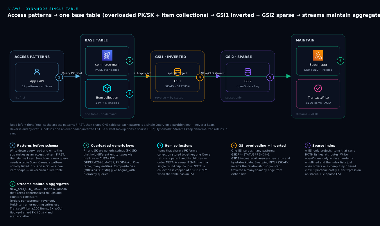
The diagram traces the model left to right: the application’s access-pattern list on the left drives everything; each pattern resolves to a single Query/Get against the base table (overloaded PK/SK, item collections), or against GSI1 (overloaded and inverted — the by-status and reverse-lookup axis) or the sparse GSI2 (only open orders). On the right, DynamoDB Streams feed a Lambda that maintains denormalized rollups and counters, while TransactWriteItems guarantees multi-item invariants like “order created and inventory decremented.” The numbered badges mark the six load-bearing ideas — patterns-first, overloaded keys, item collections, GSI overloading/inversion, the sparse index, and stream-maintained aggregates.
Real-world scenario
LedgerLeaf, a fictional but very typical B2B SaaS invoicing startup, launched on DynamoDB with a comfortable relational instinct: five tables — Accounts, Users, Invoices, LineItems, Payments — one per entity, each keyed by its own id. It shipped fast and ran fine through beta at a few hundred accounts.
The trouble began with the “Invoices” dashboard. The product needed “all overdue invoices for an account, newest first, with the customer name and total.” In the five-table model that was: Scan the Invoices table with a FilterExpression on status = OVERDUE and accountId = X, then for each result GetItem the account for its name, then for each invoice Query the LineItems table for the total. At 40,000 invoices the dashboard took 9 seconds, the Scan read every invoice on every load, and the DynamoDB bill for that one screen crossed $700/month — almost all of it capacity burned reading rows the filter immediately discarded.
The team brought in a single-table redesign. First, the access-pattern list — eleven patterns, written down for the first time. Then one table, ledger-main, with overloaded keys: PK=ACCOUNT#a1, SK=INVOICE#<ts>#<id> put every invoice in its account’s item collection, so “an account’s invoices, newest first” became one Query with ScanIndexForward=false. The customer name was denormalized onto each invoice item (snapshotted at issue time — exactly the value the invoice should show). The overdue dashboard moved to a sparse GSI: an overdue partition key written onto an invoice only while it was past due and removed on payment, so Query GSI2 PK=OVERDUE#a1 returned precisely the overdue set, reading only what it displayed. Invoice totals were pre-aggregated onto the header and kept current by a streams Lambda as line items changed.
The results were the kind that end a debate. The dashboard dropped from 9 seconds to under 120 ms. The monthly cost for that access pattern fell from ~$700 to about $18 — because the sparse GSI reads dozens of items, not tens of thousands. No Scan remained in any user-facing path. The migration itself was the hard part: a one-time backfill job re-shaped 1.4 million legacy items into the new key structure, run through a throttled BatchWriteItem pipeline over a weekend, with the app dual-reading (old table, then new) behind a feature flag until the new model was verified. The lesson the team wrote in their runbook: list the access patterns before the first CreateTable, not after the first incident.
Advantages and disadvantages
| Advantages | Disadvantages |
|---|---|
Related data fetched in one Query — no joins, no N+1 |
Steep learning curve; the model is opaque to newcomers |
| Predictable single-digit-ms latency at any scale | Rigid — new unlisted patterns can force an index or backfill |
| Fewer moving parts: one table, one IAM surface, one backup | Poor for ad-hoc/analytical queries — that is not what it is for |
| Lower cost: no over-reading, no cross-table round trips | Overloaded keys are hard to read raw; you need the entity chart |
| One transaction can span all entity types (same table) | Migrations/backfills are genuinely painful once live |
| Scales writes via sharding, reads via GSIs/DAX | Easy to over-project GSIs and quietly inflate write cost |
When each matters: the advantages dominate for known, high-volume OLTP access patterns — the invoice dashboard, the order history, the user’s feed. The disadvantages dominate when patterns are unknown, ad-hoc, or analytical — which is the entire next section.
Hands-on lab
You will build the commerce-main table with GSI1, load the entity items, run each access pattern as a real query, then add a new pattern via a sparse GSI2 on a live table — with both aws CLI and Terraform. Everything here fits the DynamoDB always-free tier (25 GB, 25 RCU/WCU or on-demand equivalents at this volume ≈ $0).
⚠️ Costs: on-demand at a few dozen requests is fractions of a cent. Adding a GSI on a large table does consume write capacity to backfill — trivial here, not on a 10 M-item table. Always run teardown (Step 8).
Step 1 — Create the base table with GSI1 (aws CLI)
aws dynamodb create-table \
  --table-name commerce-main \
  --attribute-definitions \
      AttributeName=PK,AttributeType=S \
      AttributeName=SK,AttributeType=S \
      AttributeName=GSI1PK,AttributeType=S \
      AttributeName=GSI1SK,AttributeType=S \
  --key-schema \
      AttributeName=PK,KeyType=HASH \
      AttributeName=SK,KeyType=RANGE \
  --billing-mode PAY_PER_REQUEST \
  --global-secondary-indexes \
      '[{"IndexName":"GSI1",
         "KeySchema":[{"AttributeName":"GSI1PK","KeyType":"HASH"},
                      {"AttributeName":"GSI1SK","KeyType":"RANGE"}],
         "Projection":{"ProjectionType":"ALL"}}]' \
  --region us-east-1
Only key and index attributes are declared — every other attribute is schemaless. Wait for ACTIVE:
aws dynamodb wait table-exists --table-name commerce-main --region us-east-1
Step 2 — Load the entity items
# Customer profile
aws dynamodb put-item --table-name commerce-main --item '{
  "PK":{"S":"CUST#c1"},"SK":{"S":"PROFILE"},
  "entity":{"S":"Customer"},"name":{"S":"Asha Rao"},
  "email":{"S":"asha@example.com"},"orderCount":{"N":"0"},
  "GSI1PK":{"S":"TIER#gold"},"GSI1SK":{"S":"2026-01-02"}}'

# Order header in the customer's collection (also the sparse OPEN flag)
aws dynamodb put-item --table-name commerce-main --item '{
  "PK":{"S":"CUST#c1"},"SK":{"S":"ORDER#2026-07-14#o9"},
  "entity":{"S":"Order"},"total":{"N":"59.98"},"customerName":{"S":"Asha Rao"},
  "GSI1PK":{"S":"STATUS#PENDING"},"GSI1SK":{"S":"2026-07-14T09:30Z"},
  "GSI2PK":{"S":"OPEN"}}'

# Order self-collection: header + two line items
aws dynamodb put-item --table-name commerce-main --item '{
  "PK":{"S":"ORDER#o9"},"SK":{"S":"META"},"status":{"S":"PENDING"},"total":{"N":"59.98"}}'
aws dynamodb put-item --table-name commerce-main --item '{
  "PK":{"S":"ORDER#o9"},"SK":{"S":"ITEM#sku-101"},"qty":{"N":"2"},"unitPrice":{"N":"19.99"},"name":{"S":"Clean Code"}}'
aws dynamodb put-item --table-name commerce-main --item '{
  "PK":{"S":"ORDER#o9"},"SK":{"S":"ITEM#sku-205"},"qty":{"N":"1"},"unitPrice":{"N":"20.00"},"name":{"S":"DDIA"}}'

# Product with a category axis on GSI1
aws dynamodb put-item --table-name commerce-main --item '{
  "PK":{"S":"PROD#sku-101"},"SK":{"S":"META"},"title":{"S":"Clean Code"},
  "stock":{"N":"7"},"price":{"N":"19.99"},
  "GSI1PK":{"S":"CATEGORY#books"},"GSI1SK":{"S":"PRICE#0000019.99"}}'
Step 3 — Run access patterns 1–3 (base table)
# Pattern 1: customer profile
aws dynamodb get-item --table-name commerce-main \
  --key '{"PK":{"S":"CUST#c1"},"SK":{"S":"PROFILE"}}'

# Pattern 2: a customer's orders, newest first
aws dynamodb query --table-name commerce-main \
  --key-condition-expression "PK = :pk AND begins_with(SK, :o)" \
  --expression-attribute-values '{":pk":{"S":"CUST#c1"},":o":{"S":"ORDER#"}}' \
  --no-scan-index-forward

# Pattern 3: an order with all its line items (one query, the item collection)
aws dynamodb query --table-name commerce-main \
  --key-condition-expression "PK = :pk" \
  --expression-attribute-values '{":pk":{"S":"ORDER#o9"}}'
Expected: pattern 3 returns three items — META, ITEM#sku-101, ITEM#sku-205 — in sort order, in one call. That is the item collection replacing a join.
Step 4 — Run patterns 4, 5, 8 (overloaded GSI1)
# Pattern 4: all PENDING orders (across all customers)
aws dynamodb query --table-name commerce-main --index-name GSI1 \
  --key-condition-expression "GSI1PK = :s" \
  --expression-attribute-values '{":s":{"S":"STATUS#PENDING"}}'

# Pattern 5: PENDING orders in a date window
aws dynamodb query --table-name commerce-main --index-name GSI1 \
  --key-condition-expression "GSI1PK = :s AND GSI1SK BETWEEN :a AND :b" \
  --expression-attribute-values '{":s":{"S":"STATUS#PENDING"},
     ":a":{"S":"2026-07-01"},":b":{"S":"2026-07-31"}}'

# Pattern 8: products in a category, cheapest first
aws dynamodb query --table-name commerce-main --index-name GSI1 \
  --key-condition-expression "GSI1PK = :c AND begins_with(GSI1SK, :p)" \
  --expression-attribute-values '{":c":{"S":"CATEGORY#books"},":p":{"S":"PRICE#"}}'
One index, three different questions — GSI overloading in action.
Step 5 — Add a new pattern on a live table: the sparse GSI2
Add “list only open orders” without touching existing data — only items carrying GSI2PK join the index:
aws dynamodb update-table --table-name commerce-main \
  --attribute-definitions AttributeName=GSI2PK,AttributeType=S \
  --global-secondary-index-updates \
   '[{"Create":{"IndexName":"GSI2",
       "KeySchema":[{"AttributeName":"GSI2PK","KeyType":"HASH"}],
       "Projection":{"ProjectionType":"ALL"}}}]'

aws dynamodb wait table-exists --table-name commerce-main
# Pattern 6: only open orders — the PENDING order carries GSI2PK=OPEN, the products don't
aws dynamodb query --table-name commerce-main --index-name GSI2 \
  --key-condition-expression "GSI2PK = :o" \
  --expression-attribute-values '{":o":{"S":"OPEN"}}'
Step 6 — Watch the sparse mechanic: fulfill an order
# Mark fulfilled: change status AND remove the sparse key so it leaves GSI2
aws dynamodb update-item --table-name commerce-main \
  --key '{"PK":{"S":"CUST#c1"},"SK":{"S":"ORDER#2026-07-14#o9"}}' \
  --update-expression "SET GSI1PK = :s REMOVE GSI2PK" \
  --expression-attribute-values '{":s":{"S":"STATUS#FULFILLED"}}'

# Re-run pattern 6 — the order is gone from the open-orders index
aws dynamodb query --table-name commerce-main --index-name GSI2 \
  --key-condition-expression "GSI2PK = :o" \
  --expression-attribute-values '{":o":{"S":"OPEN"}}'
Expected: the second query returns zero items — REMOVE GSI2PK dropped the order out of the sparse index without deleting anything.
Step 7 — The same table as Terraform
resource "aws_dynamodb_table" "commerce_main" {
  name         = "commerce-main"
  billing_mode = "PAY_PER_REQUEST"
  hash_key     = "PK"
  range_key    = "SK"

  attribute { name = "PK"     type = "S" }
  attribute { name = "SK"     type = "S" }
  attribute { name = "GSI1PK" type = "S" }
  attribute { name = "GSI1SK" type = "S" }
  attribute { name = "GSI2PK" type = "S" }

  global_secondary_index {
    name            = "GSI1"
    hash_key        = "GSI1PK"
    range_key       = "GSI1SK"
    projection_type = "ALL"
  }

  global_secondary_index {
    name            = "GSI2"          # sparse: only items with GSI2PK appear
    hash_key        = "GSI2PK"
    projection_type = "ALL"
  }

  stream_enabled   = true
  stream_view_type = "NEW_AND_OLD_IMAGES"   # for the aggregation Lambda

  point_in_time_recovery { enabled = true }
  server_side_encryption { enabled = true }

  ttl { attribute_name = "expiresAt", enabled = true }
}
Note the whole table is declared with just its key attributes plus the two GSIs — you never declare name, total, or stock, because DynamoDB is schemaless outside the keys. stream_view_type = NEW_AND_OLD_IMAGES wires up the delta-based aggregation path.
Step 8 — Teardown (do this)
aws dynamodb delete-table --table-name commerce-main --region us-east-1
# or, if you used Terraform:
terraform destroy -auto-approve
Common mistakes & troubleshooting
The single-table playbook. Each row: the symptom, the modeling root cause, the exact way to confirm it, and the fix.
| # | Symptom | Root cause | Confirm (exact command / path) | Fix |
|---|---|---|---|---|
| 1 | A new feature needs a Scan + FilterExpression |
An access pattern nobody listed; no key serves it | Grep code for scan(; check CloudWatch ConsumedReadCapacityUnits spikes on that call |
Add a GSI or a new item shape for the pattern — never Scan a live OLTP table |
| 2 | ValidationException: Query key condition not supported |
You put a range/begins_with on the partition key |
Read the error; inspect KeyConditionExpression |
Range conditions are legal only on the sort key; Query needs exact PK |
| 3 | Query returns fewer items than exist, LastEvaluatedKey present |
Hit the 1 MB page limit — this is normal | Response has LastEvaluatedKey |
Loop, passing ExclusiveStartKey, until it is absent — paginate |
| 4 | Hot-partition throttling despite spare table capacity | Low-cardinality PK (e.g. PK=STATUS) piles rows on one partition |
CloudWatch ThrottledRequests > 0; Contributor Insights top key |
Redesign the key for cardinality; write-shard #0..#N + scatter-gather |
| 5 | ValidationException: reserved keyword on name/status/type/data |
Attribute name collides with a DynamoDB reserved word | Check against the reserved-words list | Use ExpressionAttributeNames: #n = :v with {"#n":"name"} |
| 6 | GSI query is missing attributes you expected | GSI projection is KEYS_ONLY/INCLUDE, not ALL |
describe-table → the GSI’s Projection |
Recreate the GSI with the needed INCLUDE list (projection can’t be edited in place) |
| 7 | GSI read returns stale data right after a write | GSIs are eventually consistent, always | Compare a base GetItem (strong) vs the GSI Query |
Read the base table strongly for read-after-write; or wait out replication |
| 8 | Cannot add more than 5 local secondary indexes / can’t add an LSI later |
LSIs are fixed at table creation; you tried to add one | describe-table shows no LSI; create-table is the only place |
Use a GSI instead — addable anytime, no 10 GB collection cap |
| 9 | Item collection grew and writes fail with size errors | Table has an LSI → 10 GB per-collection limit hit | describe-table shows an LSI; watch ItemCollectionMetrics.SizeEstimateRangeGB |
Remove reliance on LSI (rebuild without it), or split the collection’s PK |
| 10 | TransactionCanceledException: ConditionalCheckFailed |
A ConditionCheck in the transaction failed (e.g. stock >= qty) |
Inspect CancellationReasons[] in the error |
Re-read current state, surface “out of stock,” retry with fresh values |
| 11 | TransactionCanceledException: TransactionConflict |
Two transactions touched the same item concurrently | Repeated conflicts under load; check CancellationReasons |
Exponential-backoff retry; reduce transaction scope; shard the contended item |
| 12 | Item size has exceeded the maximum allowed size (400 KB) |
One fat item (big list/map) crossed 400 KB | The write returns the error at ~400 KB | Vertically partition into multiple items, or store the blob in S3 + a pointer |
| 13 | Backfill/migration is slow and throttles | Rewriting millions of items into new keys saturates write capacity | BatchWriteItem returns UnprocessedItems; throttle metrics climb |
Throttled/paced pipeline, on-demand or temporary high capacity, dual-read behind a flag |
| 14 | Aggregated count/total is wrong or drifting | Denormalized rollup not kept in sync; stream consumer lag or bug | Compare rollup vs a recompute; check the stream Lambda’s iterator age/errors | Fix the stream handler idempotency; use NEW_AND_OLD_IMAGES deltas; backfill the counter |
Error / exception reference
| Error / exception | Meaning | Typical cause | Fix |
|---|---|---|---|
ValidationException |
Malformed request | Range on PK; reserved word; bad expression | Fix the key condition / use ExpressionAttributeNames |
ProvisionedThroughputExceededException |
Request rate > capacity | Hot partition or under-provisioned | Retry w/ backoff; shard key; on-demand |
ThrottlingException |
Control-plane throttle | Too many CreateTable/UpdateTable |
Backoff; batch schema changes |
ConditionalCheckFailedException |
A condition was false | Optimistic-lock or invariant failed | Re-read, decide, retry |
TransactionCanceledException |
Transaction rolled back | Condition failed or write conflict | Inspect CancellationReasons; retry conflicts |
ItemCollectionSizeLimitExceededException |
Collection > 10 GB (LSI tables) | Too many items under one PK with an LSI | Split PK; drop the LSI dependency |
ResourceInUseException |
Table busy | Modifying a CREATING/UPDATING table |
Wait for ACTIVE |
RequestLimitExceeded |
Account-level throughput limit | On-demand table hit account max | Request a limit raise before launch |
The three nastiest real failures
The Scan that hid in “just a filter.” A developer adds “search invoices by status” with Scan + FilterExpression because it works in dev with 200 items. In production with 20 million items it reads (and bills) all 20 million on every search, throttles the table, and pages the on-call. The tell is a ConsumedReadCapacity graph wildly larger than the rows returned. There is no capacity fix — only a modeling fix: a sparse or overloaded GSI so the query reads what it returns. Ban Scan from user-facing paths in code review.
The migration nobody scoped. Single-table’s dirty secret is that changing the key structure of live data means rewriting every item. Teams routinely under-estimate this: a backfill of millions of items must be paced against write capacity, made idempotent (it will be re-run), and usually paired with dual-reads behind a feature flag so the app serves the old model until the new one is verified. Model the access patterns up front precisely so you migrate rarely.
Silent aggregate drift. A stream-maintained orderCount slowly diverges from reality because the Lambda wasn’t idempotent and reprocessed some records on a retry, or its IteratorAge climbed and it fell behind. Nobody notices until a customer reports a wrong number. Guard it: idempotent handlers keyed on the event, NEW_AND_OLD_IMAGES deltas rather than blind increments, an alarm on stream IteratorAge, and a periodic reconcile job that recomputes the truth.
Best practices
- List access patterns before the first
CreateTable. The access-pattern list and entity chart are deliverables, not afterthoughts — commit them to the repo and update them with every new pattern. - Default to one table with generic
PK/SK, but do it because the patterns share access, not as dogma. Multi-table is fine when entities are genuinely unrelated. - Prefix every key value with its entity type (
CUST#,ORDER#) and carry a redundantentityattribute for stream consumers and exports. - Overload GSIs before adding new ones. One well-designed overloaded GSI beats three single-purpose ones — fewer writes, lower cost, under the 20-GSI limit.
- Reach for a sparse index whenever you would otherwise
FilterExpressiona large set down to a small, well-defined subset. - Project GSIs narrowly —
INCLUDEexactly what the pattern reads;ALLonly when the pattern truly needs the whole item. Every projected attribute is a write cost. - Prefer GSIs over LSIs. LSIs are permanent (creation-time only) and impose the 10 GB collection cap; GSIs are flexible and cap-free.
- Denormalize deliberately, and decide snapshot vs live for each copied field — freeze historical facts, stream-maintain live ones.
- Use transactions for cross-item invariants, streams for eventual aggregates. Do not pay 2× WCU for a dashboard counter, and do not risk overselling on an eventual count.
- Shard only proven-hot keys and cache the scatter-gather reads; over-sharding multiplies read cost for no benefit.
- Enable PITR, on-demand backups and TTL from day one — they are cheap insurance and a schemaless item makes TTL trivial (
expiresAtepoch).
Security notes
DynamoDB’s security model rewards the same access-pattern thinking — you can lock IAM down to item and attribute granularity, which single-table design makes especially powerful because one policy governs one table.
| Control | Mechanism | Single-table nuance |
|---|---|---|
| Encryption at rest | Always on: AWS-owned, AWS-managed (KMS), or customer-managed CMK | Choose a CMK when you need key rotation control/audit; GSIs and streams inherit it |
| Encryption in transit | TLS to the DynamoDB endpoint | Use a VPC gateway endpoint to keep traffic off the public internet (free) |
| Fine-grained access | dynamodb:LeadingKeys condition on the IAM policy |
Restrict a user to items where PK = CUST#<their-id> — multi-tenant isolation in one table |
| Attribute-level | dynamodb:Attributes + ProjectionExpression |
Let a role read only certain attributes of shared items |
| Least-privilege actions | Separate GetItem/Query from PutItem/DeleteItem/Scan |
Deny Scan in app roles entirely — it should never run on the hot path |
| Audit | CloudTrail data events for DynamoDB | Log item-level access for compliance; watch for unexpected Scan |
| Backup/DR | PITR (35 days) + on-demand backups; global tables | One table = one backup surface; restore is all-or-nothing to a new table |
The multi-tenant win is worth dwelling on: with dynamodb:LeadingKeys, an IAM policy can restrict a caller to only items whose partition key begins with their tenant id — so a single overloaded table safely serves thousands of tenants, each fenced to their own partitions, with no application-side filtering to get wrong.
Cost & sizing
DynamoDB bills for throughput (reads/writes) and storage, and single-table design bends both — usually down, because you stop over-reading. The numbers below are us-east-1, mid-2026 (WRU/RRU reflect the ~50% price cut from November 2024).
| Cost driver | On-demand price | What single-table design changes |
|---|---|---|
| Writes | WRU $0.625 / million (≤ 1 KB each) | Each GSI whose keys change adds a write — model few, narrow GSIs |
| Reads | RRU $0.125 / million (≤ 4 KB, eventually consistent) | Item collections/GSIs replace multi-read joins; no Scan over-read |
| Storage | $0.25 / GB-month after 25 GB always-free | Denormalization duplicates data — a small storage cost for join-free reads |
| Streams | $0.02 / 100k read-request units (first 2.5M free with Lambda) | Aggregation cost lives here, off the write path |
| GSI storage + writes | Same rates, per index | ALL projection copies whole items — the quiet cost leak |
| Backup (PITR) | ~$0.20 / GB-month | One table = one PITR surface |
| DAX (if used) | Per node-hour, from ~$0.04/hr (t3.small) |
Not serverless — add only for read-heavy hot paths |
| Free-tier / limits | Value |
|---|---|
| Always-free storage | 25 GB |
| Always-free throughput | 25 provisioned RCU + 25 WCU (≈ 200M req/mo) — or trivial on-demand |
| Item size | 400 KB hard max |
| Query/Scan page | 1 MB |
| GSIs per table | 20 (default, raisable) · LSIs 5 (hard) |
| Transaction | 100 items / 4 MB, 2× capacity |
| Per-partition ceiling | ~3,000 RCU / 1,000 WCU |
Worked example. The commerce workload at 5M eventually-consistent reads (≤ 4 KB) + 1M writes/month, on-demand: 5M × $0.125/M + 1M × $0.625/M ≈ $1.25/month in throughput, plus a few cents of storage under the 25 GB free tier — roughly ₹105/month. The same workload modeled as five tables with a Scan-and-filter dashboard read the whole invoice table on every dashboard load, which is exactly how LedgerLeaf’s bill reached $700; the single-table redesign returned it to single dollars. Right-sizing rule: start on-demand (zero idle cost, absorbs spikes, no throttling risk at low scale), and only move a proven steady, high-volume table to provisioned + auto-scaling once you have real traffic curves.
Interview & exam questions
Q1. Why do you model DynamoDB access-patterns-first instead of normalizing?
Because DynamoDB has no joins and no ad-hoc query planner — it guarantees performance only along the key axes you designed. Normalizing then querying leaves you with patterns no key serves, forcing Scan. You list patterns first so every one maps to a single Query/Get. (DVA-C02, SAA-C03)
Q2. What is key overloading and why do it?
Storing multiple entity types in generic PK/SK attributes, distinguished by value prefixes (CUST#, ORDER#). It collapses many entities into one table so related items share partitions, one transaction can span types, and there is one IAM/backup surface. (DVA-C02)
Q3. Explain the difference between a GSI and an LSI, and when you’d pick each. A GSI has any PK/SK, its own capacity, is eventually consistent, and can be added/removed anytime (20 max). An LSI shares the base PK and the table’s capacity, allows strong consistency, must be created with the table (5 max), and imposes a 10 GB item-collection limit. Prefer GSIs; use an LSI only when you need strong consistency on an alternate sort key. (DVA-C02, SAA-C03)
Q4. What is a sparse index and what problem does it solve?
A GSI only projects items that have both its key attributes; write the key onto just a subset and the index holds only that subset. It replaces an expensive FilterExpression (which reads and bills the whole set) with a cheap query that reads only the matching items — e.g. “open orders.” (DVA-C02)
Q5. How do you model a many-to-many relationship?
The adjacency-list pattern: store node items and edge items in one table (PK=A, SK=B for the edge). The base table gives one direction (Query PK=A); an inverted GSI (swap PK/SK) gives the other (Query GSI1PK=B). (DVA-C02)
Q6. A single partition key is throttling despite spare table capacity. Why, and what do you do?
Throughput is per partition (~1,000 WCU/3,000 RCU); one hot key can’t exceed one partition even with adaptive capacity. Confirm with Contributor Insights, then write-shard the key (#0..#N) and scatter-gather reads, or cache hot reads. (SAA-C03, DVA-C02)
Q7. How do you keep an aggregate like orders-per-customer without a Scan?
Maintain a counter attribute and update it on write — via a TransactWriteItems when it must be exact, or asynchronously via a DynamoDB Streams Lambda (ADD on insert, deltas from NEW_AND_OLD_IMAGES) when eventual consistency is acceptable. (DVA-C02)
Q8. When is single-table design the wrong choice? When access patterns are unknown or heavily ad-hoc/analytical, for small/simple apps where the modeling overhead isn’t worth it, or for reporting/aggregation workloads — route those to S3 + Athena or Redshift, or use multiple simpler tables. (SAA-C03)
Q9. What does a FilterExpression cost you, and why prefer an index?
It is applied after the read, so it reads and bills every item the key condition matched before discarding non-matches — no capacity saving. A GSI/sparse index makes the query read only the items you return. (DVA-C02)
Q10. How do item collections replace joins?
Items sharing a partition key form a collection returned by one Query. Storing an order header and its line items under the same PK returns both in a single call, ordered by sort key — the join happens at write-time modeling, not read-time. (DVA-C02)
Q11. What are the limits on a DynamoDB transaction?
TransactWriteItems/TransactGetItems handle up to 100 items and 4 MB, cost 2× the normal capacity, are serializable, and fail atomically with TransactionCanceledException (with CancellationReasons) on a condition failure or write conflict. (DVA-C02)
Q12. Why prefix and zero-pad values in sort keys?
Sort keys are strings compared lexicographically. Prefixes (ORDER#) group and order entity types within a collection; zero-padding numbers (PRICE#0000019.99) makes them sort numerically so range and begins_with queries behave. (DVA-C02)
Quick check
- You need “all orders with status = SHIPPED, newest first.” Which index technique, and what are its keys?
- Your table has an LSI and a write just failed with a size error. What limit did you hit, and what is the fix?
- Why does adding
GSI2PKto only some items create a useful index, and what is that called? - Give the base-table and inverted-GSI queries for “which users are in group g9?” in an adjacency-list model.
- When should orders-per-customer be maintained by a transaction rather than a stream?
Answers
- A sparse or overloaded GSI:
GSI1PK=STATUS#SHIPPED,GSI1SK=<timestamp>, queried withScanIndexForward=false. If SHIPPED is a transient state you filter to often, a sparse GSI keyed only while shipped is even cheaper. - The 10 GB item-collection limit, which exists because the table has an LSI. Fix: split the collection across more partition keys, or rebuild the table without the LSI (using a GSI instead).
- Because a GSI only projects items that have both its key attributes — writing
GSI2PKto just the subset you want makes the index contain only that subset. This is a sparse index. - Base:
Query PK=USER#u1, SK begins_with GROUP#for u1’s groups. Inverted GSI (PK=SK, SK=PK):Query GSI1PK=GROUP#g9for g9’s members. - When the count is part of a correctness invariant that must hold immediately (e.g. enforcing a hard cap of N orders atomically). For a dashboard number, an eventually-consistent stream-maintained counter is cheaper and sufficient.
Glossary
| Term | Definition |
|---|---|
| Single-table design | Storing multiple entity types in one DynamoDB table with generic, overloaded keys so each access pattern is one Query. |
| Access pattern | A specific read or write the application performs; the unit you design keys around. |
| Partition key (PK) | The hash key; selects the physical partition. Queried only by exact value. |
| Sort key (SK) | The range key; orders items within a partition and enables range/begins_with queries. |
| Item collection | All items sharing a partition key; returned together by one Query. |
| Key overloading | Using generic PK/SK attributes whose value prefixes encode the entity type. |
| Composite sort key | A sort key packing a hierarchy (ORG#a#DEPT#b) for multi-level begins_with queries. |
| GSI (Global Secondary Index) | An index with any PK/SK, its own capacity, eventually consistent, addable anytime (max 20). |
| LSI (Local Secondary Index) | An index sharing the base PK with an alternate SK; strong-consistent, creation-time only (max 5); imposes the 10 GB collection limit. |
| GSI overloading | Letting different entity types write different values into one GSI so it serves many patterns. |
| Inverted index | A GSI that swaps PK and SK to traverse a relationship in the reverse direction. |
| Sparse index | A GSI that projects only items carrying its key attributes — a deliberately partial, cheap view. |
| Adjacency list | Modeling nodes and edges as items in one table to represent many-to-many/graph relationships. |
| Write sharding | Spreading a hot partition key across #0..#N suffixes; reads scatter-gather across shards. |
| Denormalization | Duplicating data to avoid read-time joins; kept consistent via transactions or streams. |
| DynamoDB Streams | A 24-hour ordered change log per table; drives Lambda-maintained aggregates and copies. |
| TransactWriteItems | An all-or-nothing write of ≤ 100 items / 4 MB at 2× capacity, with per-item conditions. |
Next steps
- Ground the primitives underneath this model with DynamoDB Tables, Keys and Capacity Hands-On.
- Take the operational side further with DynamoDB Throttling and Hot-Partition Troubleshooting — the confirm-then-shard workflow in depth.
- See the table in its natural habitat in AWS Serverless Web Application Architecture.
- Wire stream-maintained aggregates into a larger system with AWS Event-Driven Architecture: EventBridge, SQS and Lambda.
- Know the boundary where you should reach for a relational engine instead in AWS Databases: RDS, DynamoDB and Aurora Compared.