The first time you meet Amazon DynamoDB it feels like a relational database with the good parts filed off: no joins, no SELECT *, no ad-hoc WHERE on any column you like, no schema to speak of. That reaction is the trap. DynamoDB is not a lesser SQL database — it is a different machine with a different contract, and once you accept the contract it gives you something no relational engine can: single-digit-millisecond reads and writes at any scale, with zero servers to patch and a bill that (done right) grows linearly with the traffic that pays for it. The price of that promise is that you must design around your access patterns, and the entire design lives in one place — the primary key.
This article is the on-ramp. You will build a real table with a composite key, put and get items, run an efficient Query and see why a Scan is the thing you avoid, add a global secondary index and query it, switch a copy of the table from on-demand to provisioned capacity with auto scaling, and turn on TTL and point-in-time recovery — all with copy-pasteable aws CLI and equivalent Terraform. Along the way you will learn the mental model that makes the rest of DynamoDB obvious: how the partition key is hashed to a physical partition, why an item is capped at 400 KB, what an RCU and a WCU actually buy you, and when a read is strongly versus eventually consistent.
Keep the tables open. Because DynamoDB is a reference-heavy service — data types, capacity math, operation limits, index rules, consistency modes — this piece is deliberately table-dense: read the prose once to build the model, then return to the tables mid-design and mid-incident. If you are still deciding whether DynamoDB is even the right store, read AWS Databases: RDS, DynamoDB and Aurora — Choose the Right Store first; this article assumes you have chosen DynamoDB and now need to wield it.
What problem this solves
Relational databases answer any question you can phrase in SQL, and they do it by scanning and joining at query time. That flexibility is a gift when queries are unpredictable and data is modest, and a liability when you need predictable low latency at scale: a join that was fast at 10 GB becomes a table-scan at 10 TB, a single writer becomes a vertical-scaling ceiling, and connection pools become a bottleneck long before storage does. DynamoDB inverts the deal. You give up query flexibility up front — you decide the access patterns before you create the table — and in return you get flat latency and horizontal scale that does not care whether the table holds a thousand items or a trillion.
What breaks without understanding this: teams treat DynamoDB like a key-value cache bolted onto relational habits. They pick a random id as the partition key, then discover they cannot list “all orders for a customer” without a full-table Scan. They put everything in one table with no sort key, then bolt on Scans with FilterExpressions and wonder why the bill and the latency both climb. They provision capacity by guessing, then either throttle during launch or pay for idle RCUs the rest of the month. Every one of these is the same root error: modelling the data instead of modelling the access patterns, and not understanding what the partition key physically does.
Who hits this: every engineer building a serverless backend (DynamoDB is the default state store behind API Gateway + Lambda serverless web apps), every team that outgrew a relational instance on a write-heavy workload, and every candidate sitting CLF-C02, DVA-C02 or SAA-C03, all of which test keys, capacity modes, indexes and consistency. The fix is to learn the machine: know what the key does, know what a read and a write cost, know when to add an index, and know the handful of failure modes cold. That is exactly what follows.
Learning objectives
By the end of this article you can:
- Explain the DynamoDB data model — tables, items, attributes — and choose between a partition-key-only and a composite (partition + sort) primary key for a given access pattern.
- Describe how the partition (hash) key is hashed to a physical partition, why that governs scale and throttling, and what the per-partition and per-item limits are.
- Use every scalar, document and set data type correctly and stay under the 400 KB item limit.
- Choose between on-demand and provisioned capacity, do the RCU/WCU math for any read or write, and configure auto scaling.
- Tell strongly from eventually consistent reads and know which operations support which.
- Run the core operations — PutItem, GetItem, UpdateItem, DeleteItem, Query, Scan, Batch, Transact — with conditional writes and optimistic locking, and know Query’s cost versus Scan’s.
- Decide between a local and a global secondary index, pick a projection, and query an index.
- Enable TTL, PITR, DynamoDB Streams, encryption and know where global tables fit.
- Diagnose the common failures —
ValidationException, empty Queries, slow Scans,ProvisionedThroughputExceeded, oversized items, missing GSI attributes, on-demand cost surprises — with the exact command to confirm and the fix.
Prerequisites & where this fits
You need an AWS account with the aws CLI v2 configured (aws configure or SSO — see AWS CLI profiles, SSO & config if that is shaky), permissions to call dynamodb:* and application-autoscaling:* in a sandbox account, and optionally Terraform 1.5+ with the aws provider. No prior NoSQL experience is assumed — if you can picture a giant hash map whose keys route to different machines, you have the intuition. Basic JSON literacy helps, because the CLI speaks DynamoDB’s typed JSON ({"S": "..."}, {"N": "42"}).
This sits at the foundation of the Databases and Serverless tracks. It is downstream of the store-selection decision in RDS, DynamoDB and Aurora compared and upstream of two deeper articles: DynamoDB single-table design & data modeling (how to fold many entity types and access patterns into one table) and DynamoDB throttling & hot-partition troubleshooting (what to do when a partition gets too hot). It pairs naturally with Lambda event-driven patterns (Streams trigger Lambda) and with S3 storage classes & lifecycle (where you offload the blobs that will not fit in a 400 KB item).
A quick map of who owns what during a DynamoDB design or incident, so you pull in the right person:
| Layer | What lives here | Who usually owns it | What it decides / can break |
|---|---|---|---|
| Data model / access patterns | Key design, GSIs, item shape | App / dev team | Whether a query is a Query or a Scan; hot partitions |
| Data-plane calls | PutItem/Query/UpdateItem, expressions | App / dev team | Latency, consumed capacity, ValidationExceptions |
| Capacity & scaling | On-demand vs provisioned, auto scaling | Platform / dev team | Throttling vs over-provisioning; the bill |
| Table features | TTL, PITR, Streams, encryption | Platform / DBA | Recovery, data lifecycle, change feed |
| Identity & network | IAM policies, VPC endpoint, KMS key | Security team | Who can read/write which items; private access |
| Cost / FinOps | Request units, storage, backups, Streams | FinOps + owners | On-demand surprises; idle provisioned capacity |
Core concepts
Start with the vocabulary, because DynamoDB reuses relational words for different things and the mismatch causes half the early confusion.
| DynamoDB term | Rough relational analogue | The important difference |
|---|---|---|
| Table | Table | No fixed schema beyond the key attributes; every item can have different attributes |
| Item | Row | A single record, ≤ 400 KB, uniquely identified by its primary key |
| Attribute | Column / field | Typed per item, not per table; can be scalar, document or set |
| Primary key | Primary key | The only mandatory structure; either partition-only or partition + sort |
| Partition key | Hash / shard key | Hashed to choose a physical partition — governs distribution |
| Sort key | Clustering key | Orders items within a partition key; enables ranges and prefixes |
| Item collection | (no direct analogue) | All items that share one partition-key value |
| Secondary index | Index | A re-projection of the table under a different key (LSI or GSI) |
| RCU / WCU | (no analogue) | The unit of read / write throughput you pay for |
| Query | Indexed SELECT … WHERE key = … |
Reads one partition efficiently by key condition |
| Scan | SELECT * FROM t (no index) |
Reads the whole table; almost always the wrong tool |
The primary key is the whole design
Every item is uniquely identified by its primary key, and DynamoDB supports exactly two shapes. Get this choice right and most queries become efficient Queries; get it wrong and you are stuck Scanning.
| Key type | Shape | Uniqueness | Access it enables | Pick it when |
|---|---|---|---|---|
| Partition key only (simple) | One attribute (HASH) | The partition key must be unique across the table | Direct lookup by that exact key only | Pure key-value: get/put by a single id (a session, a user profile by userId) |
| Composite (partition + sort) | Two attributes (HASH + RANGE) | The combination must be unique; the partition key can repeat | Get one item, or Query a range/prefix within one partition key | You need “all X for a given Y”, latest-N, ranges, or multiple item types per key |
A composite key is what you reach for the moment an access pattern says “for a customer, give me their orders” or “for a device, give me readings between two timestamps.” The partition key (CustomerId) groups related items into one item collection; the sort key (OrderId or a timestamp) orders them so a single Query returns exactly the slice you want, sorted, without reading anything else.
How the partition key maps to physical partitions
This is the single most important mechanical fact in DynamoDB. When you write an item, DynamoDB takes the partition key value, runs it through an internal hash function, and the hash output selects one physical partition — an actual storage node (backed by SSD, replicated across three Availability Zones). All items with the same partition key land on the same partition and are stored adjacent, sorted by sort key. That is why a Query by partition key is one fast, local read, and why a Scan must visit every partition.
| Fact about partitions | Value / behaviour | Why it matters |
|---|---|---|
| Selected by | hash(partition key) |
Even key distribution = even load; skewed keys = hot partition |
| Max size per partition | ~10 GB | An item collection (one PK value) that outgrows this splits — except when an LSI pins it |
| Max throughput per partition | ~3,000 RCU and ~1,000 WCU | One very hot key throttles even if the table has spare total capacity |
| Replication | 3 copies across 3 AZs | Durability and availability are automatic |
| Adaptive capacity | Automatic, instant | DynamoDB redistributes throughput toward hot partitions to a point |
| Burst capacity | Up to ~300 s of unused capacity | Absorbs short spikes before throttling |
The consequence you must internalise: choose a partition key with high cardinality and even access. A Status attribute with three values (“PLACED”, “SHIPPED”, “DELIVERED”) is a terrible partition key — three hot partitions — but a fine GSI key or sort-key prefix. A CustomerId or deviceId#date spreads load. The deep treatment of what to do when a key still runs hot lives in DynamoDB throttling & hot-partition troubleshooting; here, just remember hashing is why the key choice is physical, not cosmetic.
Data types and item structure
DynamoDB attributes are typed, and the CLI (and low-level SDK) always shows the type as a one- or two-letter descriptor wrapping the value. You will read and write this JSON constantly.
| Category | Type code | Name | Example (CLI JSON) | Notes / gotcha |
|---|---|---|---|---|
| Scalar | S |
String | {"S": "CUST#42"} |
UTF-8; can be a sort/partition key; empty string is allowed (since 2020) |
| Scalar | N |
Number | {"N": "2499.50"} |
Sent as a string; up to 38 digits of precision; can be a key |
| Scalar | B |
Binary | {"B": "dGV4dA=="} |
Base64 on the wire; can be a key |
| Scalar | BOOL |
Boolean | {"BOOL": true} |
Not a key type |
| Scalar | NULL |
Null | {"NULL": true} |
Marks an attribute explicitly null |
| Document | L |
List | {"L": [{"S":"a"},{"N":"1"}]} |
Ordered, mixed types, nestable |
| Document | M |
Map | {"M": {"k": {"S": "v"}}} |
JSON-object-like, nestable; the workhorse for nested data |
| Set | SS |
String Set | {"SS": ["a","b"]} |
Unique values, unordered, cannot be empty |
| Set | NS |
Number Set | {"NS": ["1","2"]} |
Unique numbers; no duplicates |
| Set | BS |
Binary Set | {"BS": ["dGV4dA=="]} |
Unique binaries |
Two rules trip people up. First, sets cannot be empty — removing the last element must remove the attribute, or you get a ValidationException. Second, only S, N and B may be key attributes (partition or sort); you cannot key on a boolean, list, map or set. For nested, evolving data prefer a map (M) over parallel lists.
The 400 KB item limit
Every item — the sum of all attribute names plus all values, including nested documents — must be ≤ 400 KB. This is a hard limit, not a soft quota you can raise.
| What counts toward 400 KB | Included? | Mitigation when you are close |
|---|---|---|
| Attribute values (all of them) | Yes | Compress large text (gzip → store as B) |
| Attribute names | Yes | Use short attribute names in hot items |
| Nested map/list contents | Yes | Flatten or split into multiple items in the same collection |
| Number of attributes | No hard cap, but size is | Vertical-split a wide item across sort-key “facets” |
| Large binary blobs (images, PDFs) | Yes | Store the blob in S3 and keep only the S3 key in DynamoDB |
The idiomatic pattern for big payloads is the S3 pointer: put the object in S3, store s3://bucket/key (and metadata) in the item. DynamoDB stays small and fast; S3 holds the bytes. Trying to cram a 2 MB document into an item is the wrong shape and will fail on write.
Capacity modes: on-demand vs provisioned
Every table runs in one of two capacity modes, and this is the choice that most directly shapes both your operational burden and your bill. You can switch modes, but only once every 24 hours per table.
| Dimension | On-demand (PAY_PER_REQUEST) | Provisioned (PROVISIONED) |
|---|---|---|
| You configure | Nothing (optionally a max throughput) | RCUs and WCUs (with optional auto scaling) |
| Billing unit | Per request: RRU / WRU | Per hour of provisioned RCU / WCU |
| Handles spikes | Instantly, up to 2× previous peak; higher via pre-warming | Only up to provisioned + burst; else throttles |
| Throttling risk | Very low (unless you exceed table limits) | High if under-provisioned |
| Cost profile | Higher per request; zero when idle | Cheaper per request at steady load; pay even when idle |
| Free-tier eligible | No always-free allotment | Yes: 25 RCU + 25 WCU always free |
| Best for | Spiky, unpredictable, new, or dev/test workloads | Steady, predictable, high-volume production traffic |
| Auto scaling | N/A (it is inherently elastic) | Optional target-tracking auto scaling |
Rule of thumb: start on-demand. It removes an entire class of throttling incidents while you are still learning the traffic shape. Once traffic is steady and understood, provisioned with auto scaling is usually cheaper. A workload with a flat baseline and rare spikes can even sit provisioned-with-auto-scaling and let the policy chase the curve.
The RCU / WCU math (know this cold)
Capacity is metered in read capacity units (RCU) and write capacity units (WCU) for provisioned, and the equivalent per-request read/write request units (RRU/WRU) for on-demand. The conversion rules are the most-tested numbers in the whole service.
| Unit | Buys you | Rounding | Consistency multiplier |
|---|---|---|---|
| 1 RCU | 1 strongly-consistent read/sec of an item up to 4 KB | Round item size up to next 4 KB | Eventually consistent = ½ RCU; transactional = 2 RCU |
| 1 WCU | 1 write/sec of an item up to 1 KB | Round item size up to next 1 KB | Transactional write = 2 WCU |
| 1 RRU (on-demand) | 1 strongly-consistent read up to 4 KB | Same 4 KB rounding | Eventually consistent = ½ RRU; transactional = 2 RRU |
| 1 WRU (on-demand) | 1 write up to 1 KB | Same 1 KB rounding | Transactional = 2 WRU |
Worked read examples — how many RCUs one read consumes:
| Read | Item size | Consistency | RCU cost | Why |
|---|---|---|---|---|
| GetItem | 3 KB | Strong | 1 | Rounds up to 4 KB → 1 unit |
| GetItem | 3 KB | Eventual | 0.5 | Half of strong |
| GetItem | 8 KB | Strong | 2 | 8 KB ÷ 4 KB = 2 |
| GetItem | 8 KB | Eventual | 1 | Half of 2 |
| GetItem | 12 KB | Strong | 3 | 12 KB ÷ 4 KB = 3 |
| GetItem | 0.5 KB | Strong | 1 | Minimum 4 KB rounding |
| TransactGetItems | 4 KB | Transactional | 2 | 2× strong |
| Query returning 40 KB | 40 KB total | Eventual | 5 | 40 ÷ 4 = 10, ½ = 5 (billed on total read, pre-filter) |
Worked write examples — how many WCUs one write consumes:
| Write | Item size | Type | WCU cost | Why |
|---|---|---|---|---|
| PutItem | 0.5 KB | Standard | 1 | Rounds up to 1 KB |
| PutItem | 1 KB | Standard | 1 | Exactly 1 unit |
| PutItem | 2.5 KB | Standard | 3 | Rounds up to 3 KB → 3 units |
| UpdateItem | 3 KB item | Standard | 3 | Charged on the full new item size, not the delta |
| DeleteItem | 1 KB | Standard | 1 | Delete costs a write of the item size |
| TransactWriteItems | 1 KB | Transactional | 2 | 2× standard |
| PutItem 1 KB + 1 GSI | 1 KB base | Standard | 1 (base) + 1 (GSI) | Each projected GSI write is billed separately |
To size provisioned throughput: to sustain N strongly-consistent 4 KB reads per second, provision N RCUs; for eventually consistent, provision N/2. To sustain M 1 KB writes per second, provision M WCUs. Two subtleties that cost people money: a Query or Scan is billed on the total size of items read before any FilterExpression (filtering does not save capacity), and an UpdateItem is billed on the size of the whole resulting item, not the changed bytes.
Auto scaling for provisioned tables
Provisioned tables can auto-scale via Application Auto Scaling target-tracking: you set a target utilisation and min/max bounds, and DynamoDB adjusts capacity to keep consumed/provisioned near the target.
| Auto scaling setting | Typical value | Effect / gotcha |
|---|---|---|
| Target utilisation | 70% | Higher = cheaper but less headroom for spikes |
| Min capacity | Your steady-state floor | Too low = throttles at the start of a ramp |
| Max capacity | Spike ceiling + margin | The real cap; scaling never exceeds it |
| Scale-out speed | Fast (seconds–minutes) | Handles gradual ramps well |
| Scale-in speed | Slow, conservative | Avoids flapping; you keep paying briefly after a spike |
| Applies to | Table and each GSI separately | A GSI can throttle independently — scale it too |
Auto scaling reacts to sustained change, not instantaneous bursts. For a known spike (a sale launch, a batch import) either pre-provision, switch to on-demand for the window, or raise the min ahead of time — do not rely on the policy to catch a step-function of traffic.
Consistency, reads and writes
DynamoDB replicates every write across three AZs. A read can either wait for a majority (strong) or accept whatever the nearest replica has (eventual, the default).
| Read mode | Flag | Latency | Cost | Guarantee | Where available |
|---|---|---|---|---|---|
| Eventually consistent | default | Lowest | ½ RCU | May not reflect a write from the last ~1 second | Everywhere, including GSIs |
| Strongly consistent | --consistent-read |
Slightly higher | 1 RCU | Reflects all successful prior writes | Base table + LSI only — never on a GSI |
| Transactional | Transact APIs | Highest | 2 RCU | ACID across up to 100 items | TransactGetItems/TransactWriteItems |
The rule to memorise for exams and incidents: a global secondary index is always eventually consistent — you cannot ask a GSI for a strongly-consistent read. If your read-after-write test queries a GSI and “loses” the item, that is by design (see the troubleshooting playbook). Writes are always durable once acknowledged; the choice is only on the read side.
Operations: the data-plane API
DynamoDB’s data plane is a small, sharp set of calls. Learn what each one costs and which access pattern it serves.
| Operation | What it does | Reads/writes | Capacity model | Consistency options |
|---|---|---|---|---|
| PutItem | Create or fully replace one item | Write | 1 write of new item size | Conditional via ConditionExpression |
| GetItem | Fetch one item by full primary key | Read | 1 read of item size | Eventual or strong |
| UpdateItem | Modify attributes of one item (upsert) | Write | 1 write of resulting item size | Conditional; atomic counters |
| DeleteItem | Remove one item by primary key | Write | 1 write of item size | Conditional |
| Query | Read items sharing a partition key, by key condition | Read | Total size read (pre-filter) | Eventual or strong (not on GSI) |
| Scan | Read every item in a table/index | Read | Total size of everything scanned | Eventual or strong |
| BatchGetItem | Up to 100 items / 16 MB across tables | Read | Sum of item reads | Per-item eventual or strong |
| BatchWriteItem | Up to 25 puts/deletes / 16 MB | Write | Sum of item writes | No conditions, no updates |
| TransactWriteItems | Up to 100 writes, all-or-nothing | Write | 2× per item | ACID; ConditionCheck supported |
| TransactGetItems | Up to 100 reads, consistent snapshot | Read | 2× per item | ACID snapshot |
Query vs Scan — the cost that decides careers
This is the difference between a system that scales and one that falls over. A Query targets one partition key and reads only the matching item collection (optionally narrowed by a sort-key condition). A Scan reads the entire table, page by page, and applies any filter after reading — so you pay for every byte even for items you throw away.
| Aspect | Query | Scan |
|---|---|---|
| Reads | One partition key’s items | Every item in the table/index |
| Requires | Partition key = condition |
Nothing |
| Sort-key conditions | =, <, <=, >, >=, BETWEEN, begins_with |
N/A |
| Cost | Proportional to items returned | Proportional to table size |
| Latency at scale | Flat | Grows with the table |
| Page size | Up to 1 MB per call, then paginate | Up to 1 MB per call, then paginate |
| FilterExpression | Narrows results, not cost | Narrows results, not cost |
| When acceptable | Almost always | Rare: small tables, admin exports, or parallel Scan for full re-index |
If you find yourself Scanning in a hot path, the fix is not a bigger Scan — it is a better key or a GSI so the pattern becomes a Query. That redesign is the subject of DynamoDB single-table design.
Sort-key condition expressions
Within a Query, the sort-key condition is what turns “all of a customer’s orders” into “this customer’s July orders” or “their latest three.”
| Sort-key condition | Example | Returns |
|---|---|---|
= |
OrderId = :id |
One exact item |
<, <=, >, >= |
CreatedAt >= :t |
Items on one side of a boundary |
BETWEEN … AND … |
CreatedAt BETWEEN :a AND :b |
An inclusive range |
begins_with(...) |
begins_with(OrderId, :prefix) |
A prefix slice (great for hierarchical keys) |
| (none) | partition key only | The whole item collection |
Add --no-scan-index-forward to read a range in descending sort order (newest first), and --limit N to cap the page — together they express “latest N” cheaply.
Conditional writes, expressions and optimistic locking
Every write can carry a ConditionExpression that must be true or the write fails with ConditionalCheckFailedException (and consumes capacity but changes nothing). This is how you get correctness without read-modify-write races.
| Pattern | Expression | Guards against |
|---|---|---|
| Create-if-absent | attribute_not_exists(OrderId) |
Overwriting an existing item on PutItem |
| Update-if-present | attribute_exists(OrderId) |
Creating a ghost item on UpdateItem |
| Optimistic locking | Version = :expected |
Lost updates under concurrency |
| State-machine guard | #s = :from (Status = “PLACED”) |
Illegal transitions (ship a cancelled order) |
| Idempotency | attribute_not_exists(RequestId) |
Double-processing a retried request |
Optimistic locking is worth internalising: store a Version number on the item, and on every UpdateItem both bump it (SET Version = Version + :one) and require the old value (ConditionExpression: Version = :cur). Two concurrent writers race; one wins, the other gets ConditionalCheckFailedException and re-reads. No pessimistic locks, no deadlocks.
Update expressions themselves are a small language:
| Update clause | Example | Effect |
|---|---|---|
SET |
SET #s = :new |
Assign / overwrite an attribute |
SET + arithmetic |
SET Views = Views + :one |
Atomic counter increment |
REMOVE |
REMOVE OldFlag |
Delete an attribute |
ADD |
ADD Score :n |
Numeric add or add-to-set (legacy but useful) |
DELETE |
DELETE Tags :t |
Remove elements from a set |
list_append |
SET Items = list_append(Items, :more) |
Append to a list |
if_not_exists |
SET Count = if_not_exists(Count, :zero) + :one |
Initialise-then-increment safely |
Because many natural attribute names (Status, Name, Size, Count, Timestamp, Data) are reserved words, you alias them with ExpressionAttributeNames (#s) and always pass values via ExpressionAttributeValues (:new). Doing this by default avoids a whole category of ValidationException.
Batch vs transaction limits
| Operation | Max items | Max size | Atomic? | Conditions? | Updates? |
|---|---|---|---|---|---|
| BatchGetItem | 100 | 16 MB | No (per-item) | No | N/A |
| BatchWriteItem | 25 | 16 MB | No (per-item) | No | No (put/delete only) |
| TransactWriteItems | 100 | 4 MB | Yes (all-or-nothing) | Yes | Yes |
| TransactGetItems | 100 | 4 MB | Yes (snapshot) | N/A | N/A |
Batches can return UnprocessedItems / UnprocessedKeys under throttling — you must retry those with backoff; the SDK does not always do it for you. Transactions are all-or-nothing and cost double, so use them only where you truly need cross-item atomicity (transfer money, reserve inventory), not as a default write path.
Secondary indexes: LSI vs GSI
An index lets you query the same data by a different key. DynamoDB has two kinds, and choosing wrong is expensive because an LSI can only be created with the table.
| Attribute | Local Secondary Index (LSI) | Global Secondary Index (GSI) |
|---|---|---|
| Partition key | Same as the table | Any attribute (different from table) |
| Sort key | A different attribute | Any attribute |
| When created | Only at table creation | Any time, added/removed live |
| Max per table | 5 | 20 (default soft limit) |
| Throughput | Shares the table’s capacity | Own capacity (or on-demand) |
| Consistency | Strong or eventual | Eventual only |
| Size limit impact | Caps item collection at 10 GB per PK | No item-collection cap |
| Keys must exist? | Item indexed only if it has the sort key | Item indexed only if it has both index keys |
Decision table:
| If you need… | Use | Because |
|---|---|---|
| Another sort order for the same partition key, with strong reads | LSI | Only LSI shares the partition and allows strong consistency |
| A query by a completely different attribute | GSI | GSI can re-partition on any attribute |
| To add the index to a live table | GSI | LSIs cannot be added after creation |
| Isolated throughput for the index workload | GSI | GSI has its own RCU/WCU |
| To avoid the 10 GB per-partition cap | GSI | LSI imposes the 10 GB item-collection limit |
Projections — what the index carries
A GSI does not copy the whole item; you choose a projection, and querying a non-projected attribute forces an extra fetch from the base table (or returns nothing if you filtered on it).
| Projection type | Copies into the index | Use when | Trade-off |
|---|---|---|---|
KEYS_ONLY |
Base + index keys only | You only need to find keys, then GetItem the rest | Smallest/cheapest index; extra read to hydrate |
INCLUDE |
Keys + a named attribute list | You need a few specific fields on the query | Balance of size vs completeness |
ALL |
Every attribute | The query needs the full item | Largest index; ~2× storage & write cost |
A GSI is a materialised copy kept up to date asynchronously: every base write that touches projected attributes triggers a write to the index (billed separately, hence “GSI own capacity”). Under-provision the GSI and you throttle the base-table writes — a classic surprise covered in the playbook.
Table features: TTL, PITR, Streams, encryption, global tables
Beyond keys and capacity, a handful of table-level features turn a bare key-value store into a production data layer.
| Feature | What it does | Cost | Key limit / behaviour |
|---|---|---|---|
| TTL | Auto-deletes items past an epoch timestamp attribute | Free (deletes don’t cost WCU) | Deletion within ~48 h of expiry, not instant |
| Point-in-time recovery (PITR) | Continuous backups; restore to any second | Per-GB-month of backup | Rolling 35-day window; restores to a new table |
| On-demand backup | Full, retained snapshot | Per-GB-month | Kept until you delete it; no performance impact |
| DynamoDB Streams | Ordered change feed of item modifications | Per read request | 24-hour retention; per-shard ordering |
| Encryption at rest | AES-256 via KMS, always on | Owned key free; managed/CMK billed | Cannot be disabled |
| Global tables | Multi-Region, multi-active replication | Cross-Region replicated writes (rWCU) | Requires Streams; last-writer-wins |
TTL specifics
| TTL detail | Behaviour |
|---|---|
| Attribute format | A Number holding a Unix epoch time in seconds (not milliseconds) |
| Timing | Background delete, typically within 48 hours of expiry — not real-time |
| Reads before delete | Expired-but-not-yet-deleted items can still be returned — filter in the app if precision matters |
| Streams | TTL deletes appear in Streams (with userIdentity = dynamodb, principal dynamodb.amazonaws.com) |
| Cost | The deletes themselves consume no write capacity |
TTL is how you keep tables lean — expire sessions, carts, verification codes, event logs — without a nightly cleanup job. Because it is eventual, never rely on it for correctness (a security token must be validated by its own expiry field, not merely “trusted to be gone”).
DynamoDB Streams view types
DynamoDB Streams emit an ordered, per-partition-key feed of every write; a Lambda function or Kinesis consumer reacts to it. This is the backbone of event-driven data flows — see Lambda event-driven patterns.
| StreamViewType | Record contains | Use for |
|---|---|---|
KEYS_ONLY |
Just the changed item’s keys | “Something changed here” fan-out |
NEW_IMAGE |
The item after the change | Replicating current state, search indexing |
OLD_IMAGE |
The item before the change | Auditing what was removed/overwritten |
NEW_AND_OLD_IMAGES |
Both before and after | Change-data-capture, diffs, most flexible |
For encryption, DynamoDB gives you three key options: the default AWS owned key (free, invisible), the AWS managed key aws/dynamodb, or a customer-managed key (CMK) for full control and its own key policy — the CMK path is what compliance-driven workloads pick. Global tables are the multi-Region story: they replicate a table to other Regions with active-active writes and last-writer-wins conflict resolution, giving low local latency and Regional failover; they build on Streams and are a topic in their own right.
Architecture at a glance
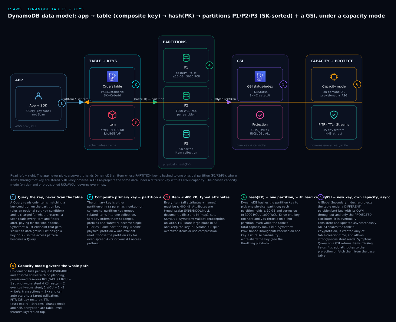
The diagram below is the mental model to burn in. Read it left to right: your app never chooses a server — it hands DynamoDB an item, and the partition key is hashed to route that item to exactly one physical partition (P1/P2/P3), where items sharing the key are stored sort-key ordered. A global secondary index re-projects the same data under a different key with its own capacity, updated asynchronously. The capacity mode you chose (on-demand or provisioned RCU/WCU) governs the cost and throttling of every hop, while table features (TTL, PITR, Streams, KMS) sit alongside. The numbered badges mark the six decisions that make or break the design — from “Query, never Scan” at the app, through the composite key and the per-partition ceilings, to the GSI’s own capacity and the capacity mode that prices it all.
Real-world scenario
ShopFleet, a fictional D2C retailer, launched an order-tracking service on DynamoDB and nearly torched it on their first flash sale. The original table used OrderId as a partition-key-only primary key — clean for GetItem(orderId), useless for the app’s real hottest query: “show me all of a customer’s orders, newest first.” Engineering had implemented that screen as a Scan with a FilterExpression on CustomerId. At 40,000 orders it was tolerable. At 6 million it read the whole table on every page load, consumed thousands of RRUs per request, and the “My Orders” page took 9 seconds.
The redesign was a keying change, not a rewrite. They created a new table with a composite key: partition key CustomerId, sort key OrderId encoded as ORDER#<date>#<seq> so it sorts chronologically. “All orders for a customer, newest first” became a single Query with --no-scan-index-forward and --limit 20 — a few RCUs, 8 ms, flat regardless of table size. For the ops team’s “all PLACED orders across everyone” screen they added a GSI status-index (partition key Status, sort key CreatedAt) with an INCLUDE projection of Amount and CustomerId, so the fulfilment dashboard queries the index directly without touching the base table’s capacity.
They left the table on-demand through the migration and the next sale — no capacity guessing while traffic was unknown. Post-sale analytics showed a stable daily curve (a predictable morning ramp, a flat plateau, a quiet night), so they moved the base table to provisioned with auto scaling: min 200 WCU / 400 RCU, max 4,000 each, target 70%. The GSI got its own auto-scaling policy because the fulfilment dashboard’s read pattern is spikier than the write path. They enabled PITR the day they went live (a one-line change that would have saved them during a bad bulk-update the previous quarter) and set TTL on a separate EventLog table so per-order audit events self-expire after 90 days instead of accumulating forever.
The measurable outcome:
| Metric | Before (Scan on wrong key) | After (Query + GSI) |
|---|---|---|
| “My Orders” latency (p95) | 9,000 ms | 8 ms |
| Read units per page load | ~3,100 RRU | ~6 RRU |
| Behaviour at 10× data | Linear slowdown | Flat |
| Fulfilment dashboard | Scan of base table | GSI Query, isolated capacity |
| Monthly DynamoDB spend | Spiking, unpredictable | ~55% lower, predictable |
| Recovery from bad write | None (no backups) | PITR to any second in 35 days |
The lesson ShopFleet took away is the lesson of this article: the partition key is the design. A one-attribute keying mistake turned every read into a table Scan; a one-attribute keying fix turned it into an indexed Query.
Advantages and disadvantages
| Advantages | Disadvantages |
|---|---|
| Single-digit-ms latency at any scale | Access patterns must be designed up front |
| Fully serverless — no patching, no instances | No ad-hoc queries, no joins, no SELECT * |
| Horizontal scale with even keys, effectively unbounded | A skewed key throttles (hot partition) |
| On-demand absorbs spikes with zero planning | On-demand can surprise you on cost at high volume |
| Fine-grained IAM down to the item/attribute | 400 KB item cap; large blobs must live in S3 |
| Built-in PITR, TTL, Streams, encryption, global tables | GSIs cost extra storage + write capacity |
| Predictable, linear cost at steady provisioned load | Provisioned under-sizing throttles; over-sizing wastes |
| ACID transactions when you need them | Transactions cost 2× and cap at 100 items |
When each matters: the advantages dominate for high-scale, well-understood, key-addressable workloads (carts, sessions, user profiles, IoT telemetry, event stores, order tracking). The disadvantages bite hardest for reporting, analytics and exploratory query workloads — for those, either add a GSI per known pattern, stream to a system built for ad-hoc query (Athena over S3, OpenSearch), or reconsider whether a relational store from the RDS/Aurora comparison fits better.
Hands-on lab
A complete, free-tier-friendly walk-through: create a composite-key table on-demand, write and read items, run a Query and see why Scan is worse, add and query a GSI, switch a copy to provisioned with auto scaling, enable TTL and PITR, then tear it all down. Everything runs in us-east-1; swap the Region if you prefer. ⚠️ On-demand requests and provisioned capacity beyond the 25 RCU/25 WCU always-free tier cost a few cents at this volume — the teardown at the end removes everything.
Step 1 — Create the table (composite key, on-demand).
aws dynamodb create-table \
  --table-name Orders \
  --attribute-definitions \
      AttributeName=CustomerId,AttributeType=S \
      AttributeName=OrderId,AttributeType=S \
  --key-schema \
      AttributeName=CustomerId,KeyType=HASH \
      AttributeName=OrderId,KeyType=RANGE \
  --billing-mode PAY_PER_REQUEST \
  --tags Key=env,Value=lab \
  --region us-east-1

aws dynamodb wait table-exists --table-name Orders
Expected: create-table returns the table description with "TableStatus": "CREATING"; the wait call blocks until it flips to ACTIVE, then returns silently.
Step 2 — Put a few items (with a create-if-absent guard).
aws dynamodb put-item --table-name Orders \
  --item '{
    "CustomerId": {"S": "CUST#42"},
    "OrderId":    {"S": "ORDER#2026-07-14#1001"},
    "Status":     {"S": "PLACED"},
    "Amount":     {"N": "2499"},
    "CreatedAt":  {"S": "2026-07-14T10:30:00Z"},
    "Version":    {"N": "1"}
  }' \
  --condition-expression "attribute_not_exists(OrderId)"

aws dynamodb put-item --table-name Orders \
  --item '{ "CustomerId": {"S": "CUST#42"}, "OrderId": {"S": "ORDER#2026-07-14#1002"},
            "Status": {"S": "PLACED"}, "Amount": {"N": "899"},
            "CreatedAt": {"S": "2026-07-14T11:05:00Z"}, "Version": {"N": "1"} }'
Expected: no output on success. Re-running the first command returns An error occurred (ConditionalCheckFailedException) — proof the guard works.
Step 3 — Get one item, strongly consistent, and see the cost.
aws dynamodb get-item --table-name Orders \
  --key '{"CustomerId": {"S": "CUST#42"}, "OrderId": {"S": "ORDER#2026-07-14#1001"}}' \
  --consistent-read \
  --return-consumed-capacity TOTAL
Expected: the item JSON plus "ConsumedCapacity": {"TableName": "Orders", "CapacityUnits": 1.0} — a small item, strong read, exactly 1 RCU.
Step 4 — Query the customer’s orders, newest first (the efficient path).
aws dynamodb query --table-name Orders \
  --key-condition-expression "CustomerId = :c AND begins_with(OrderId, :p)" \
  --expression-attribute-values '{":c": {"S": "CUST#42"}, ":p": {"S": "ORDER#2026-07"}}' \
  --no-scan-index-forward \
  --return-consumed-capacity TOTAL
Expected: both July orders, newest first, with CapacityUnits around 0.5 (small items, eventual read). This is the pattern to internalise: one partition key, a sort-key prefix, sorted, cheap.
Step 5 — Contrast with a Scan (the anti-pattern) and watch the cost.
aws dynamodb scan --table-name Orders \
  --filter-expression "#s = :st" \
  --expression-attribute-names '{"#s": "Status"}' \
  --expression-attribute-values '{":st": {"S": "PLACED"}}' \
  --return-consumed-capacity TOTAL
Expected: the same items, but the consumed capacity reflects every item read before the filter. On a two-item table the difference is trivial; imagine it at 6 million items and you understand ShopFleet’s 9-second page.
Step 6 — Add a GSI and query by Status.
aws dynamodb update-table --table-name Orders \
  --attribute-definitions \
      AttributeName=Status,AttributeType=S \
      AttributeName=CreatedAt,AttributeType=S \
  --global-secondary-index-updates '[{
    "Create": {
      "IndexName": "status-index",
      "KeySchema": [
        {"AttributeName": "Status",    "KeyType": "HASH"},
        {"AttributeName": "CreatedAt", "KeyType": "RANGE"}
      ],
      "Projection": {"ProjectionType": "INCLUDE", "NonKeyAttributes": ["Amount", "CustomerId"]}
    }
  }]'

aws dynamodb wait table-exists --table-name Orders   # index backfill runs async

aws dynamodb query --table-name Orders --index-name status-index \
  --key-condition-expression "#s = :st" \
  --expression-attribute-names '{"#s": "Status"}' \
  --expression-attribute-values '{":st": {"S": "PLACED"}}' \
  --return-consumed-capacity TOTAL
Expected: the GSI query returns both PLACED orders with only the projected attributes (Amount, CustomerId, plus the keys). Note the index takes a moment to backfill; a query immediately after creation may return fewer items until IndexStatus is ACTIVE (check with describe-table).
Step 7 — Update with an atomic counter and optimistic lock.
aws dynamodb update-item --table-name Orders \
  --key '{"CustomerId": {"S": "CUST#42"}, "OrderId": {"S": "ORDER#2026-07-14#1001"}}' \
  --update-expression "SET #s = :new ADD Version :one" \
  --condition-expression "Version = :cur" \
  --expression-attribute-names '{"#s": "Status"}' \
  --expression-attribute-values '{":new": {"S": "SHIPPED"}, ":one": {"N": "1"}, ":cur": {"N": "1"}}' \
  --return-values ALL_NEW
Expected: the updated item with Status: SHIPPED and Version: 2. Run it again unchanged and it fails with ConditionalCheckFailedException because Version is now 2, not 1 — optimistic locking in action.
Step 8 — Switch a COPY to provisioned + auto scaling. Do not flip the live table (mode changes are limited to once per 24 h and this keeps the lab reversible). Create a second table provisioned:
aws dynamodb create-table --table-name OrdersProvisioned \
  --attribute-definitions AttributeName=CustomerId,AttributeType=S AttributeName=OrderId,AttributeType=S \
  --key-schema AttributeName=CustomerId,KeyType=HASH AttributeName=OrderId,KeyType=RANGE \
  --billing-mode PROVISIONED \
  --provisioned-throughput ReadCapacityUnits=5,WriteCapacityUnits=5
aws dynamodb wait table-exists --table-name OrdersProvisioned

aws application-autoscaling register-scalable-target \
  --service-namespace dynamodb --resource-id "table/OrdersProvisioned" \
  --scalable-dimension "dynamodb:table:WriteCapacityUnits" \
  --min-capacity 5 --max-capacity 100

aws application-autoscaling put-scaling-policy \
  --service-namespace dynamodb --resource-id "table/OrdersProvisioned" \
  --scalable-dimension "dynamodb:table:WriteCapacityUnits" \
  --policy-name "orders-write-tt" --policy-type TargetTrackingScaling \
  --target-tracking-scaling-policy-configuration '{
    "TargetValue": 70.0,
    "PredefinedMetricSpecification": {"PredefinedMetricType": "DynamoDBWriteCapacityUtilization"}
  }'
Expected: the scalable target and policy register; from now on write capacity tracks 70% utilisation between 5 and 100 WCU. (Repeat the two Application Auto Scaling calls with ReadCapacityUnits / DynamoDBReadCapacityUtilization to scale reads too.)
Step 9 — Enable TTL and PITR on the main table.
aws dynamodb update-time-to-live --table-name Orders \
  --time-to-live-specification "Enabled=true,AttributeName=ExpiresAt"

aws dynamodb update-continuous-backups --table-name Orders \
  --point-in-time-recovery-specification PointInTimeRecoveryEnabled=true
Expected: TTL returns "TimeToLiveStatus": "ENABLING"; PITR returns "PointInTimeRecoveryStatus": "ENABLED". Any item you now write with an ExpiresAt number (epoch seconds in the past) will be background-deleted within ~48 hours.
Step 10 — Teardown (⚠️ deletes everything, stops all charges).
aws application-autoscaling deregister-scalable-target \
  --service-namespace dynamodb --resource-id "table/OrdersProvisioned" \
  --scalable-dimension "dynamodb:table:WriteCapacityUnits"

aws dynamodb delete-table --table-name OrdersProvisioned
aws dynamodb delete-table --table-name Orders
aws dynamodb wait table-not-exists --table-name Orders
aws dynamodb wait table-not-exists --table-name OrdersProvisioned
Deleting a table drops its GSIs, Streams, TTL config and PITR settings with it. Confirm with aws dynamodb list-tables — neither table should appear.
The whole lab as Terraform
The same result declaratively. main_table is on-demand with a GSI, TTL, PITR, Streams and encryption; provisioned_table shows provisioned mode with a target-tracking auto-scaling policy.
resource "aws_dynamodb_table" "main_table" {
  name         = "Orders"
  billing_mode = "PAY_PER_REQUEST"
  hash_key     = "CustomerId"
  range_key    = "OrderId"

  attribute { name = "CustomerId" type = "S" }
  attribute { name = "OrderId"    type = "S" }
  attribute { name = "Status"     type = "S" }
  attribute { name = "CreatedAt"  type = "S" }

  global_secondary_index {
    name               = "status-index"
    hash_key           = "Status"
    range_key          = "CreatedAt"
    projection_type    = "INCLUDE"
    non_key_attributes = ["Amount", "CustomerId"]
  }

  ttl {
    attribute_name = "ExpiresAt"
    enabled        = true
  }

  point_in_time_recovery { enabled = true }

  server_side_encryption { enabled = true } # AWS managed KMS key aws/dynamodb

  stream_enabled   = true
  stream_view_type = "NEW_AND_OLD_IMAGES"

  tags = { env = "lab" }
}

resource "aws_dynamodb_table" "provisioned_table" {
  name           = "OrdersProvisioned"
  billing_mode   = "PROVISIONED"
  read_capacity  = 5
  write_capacity = 5
  hash_key       = "CustomerId"
  range_key      = "OrderId"

  attribute { name = "CustomerId" type = "S" }
  attribute { name = "OrderId"    type = "S" }
}

resource "aws_appautoscaling_target" "write" {
  max_capacity       = 100
  min_capacity       = 5
  resource_id        = "table/${aws_dynamodb_table.provisioned_table.name}"
  scalable_dimension = "dynamodb:table:WriteCapacityUnits"
  service_namespace  = "dynamodb"
}

resource "aws_appautoscaling_policy" "write" {
  name               = "orders-write-tt"
  policy_type        = "TargetTrackingScaling"
  resource_id        = aws_appautoscaling_target.write.resource_id
  scalable_dimension = aws_appautoscaling_target.write.scalable_dimension
  service_namespace  = aws_appautoscaling_target.write.service_namespace

  target_tracking_scaling_policy_configuration {
    predefined_metric_specification {
      predefined_metric_type = "DynamoDBWriteCapacityUtilization"
    }
    target_value = 70
  }
}
terraform apply builds it; terraform destroy is your teardown. Note that in Terraform you only declare an attribute {} block for attributes used as a table or index key — never for ordinary data attributes, a point the troubleshooting section returns to.
Common mistakes & troubleshooting
DynamoDB fails in a small, learnable set of ways. Here is the playbook — symptom, root cause, the exact command or console path to confirm it, and the fix.
| # | Symptom | Root cause | Confirm (command / console) | Fix |
|---|---|---|---|---|
| 1 | ValidationException: One or more parameter values were invalid: Missing the key CustomerId |
PutItem/GetItem omitted a key attribute | Re-read the error; aws dynamodb describe-table --table-name Orders --query 'Table.KeySchema' |
Include every key attribute (both PK and SK for a composite key) in --item / --key |
| 2 | ValidationException: Type mismatch for key CustomerId expected: S actual: N |
Wrong attribute type sent for a key | describe-table → AttributeDefinitions |
Send the declared type ({"S": …} not {"N": …}); types are fixed at creation |
| 3 | ValidationException: Attribute name is a reserved keyword; reserved keyword: Status |
Used a reserved word directly in an expression | Check the AWS reserved-words list | Alias with ExpressionAttributeNames (#s) and reference #s |
| 4 | Query returns zero items but the data exists | Wrong key condition — e.g. filtering on a non-key, or using = where a prefix was needed |
Run the Query with --return-consumed-capacity TOTAL; verify the PK value exactly |
Query must include partition key =; use begins_with/BETWEEN on the sort key, not a FilterExpression on the partition key |
| 5 | Query on a GSI “loses” a just-written item | GSIs are eventually consistent and update asynchronously | Repeat the query after ~1 s; GetItem the base table (strong) confirms the write landed | Don’t read-after-write on a GSI; query the base table for immediate consistency |
| 6 | GSI query returns items missing attributes | The attribute isn’t in the index projection | describe-table → the index Projection |
Recreate/extend the GSI with INCLUDE/ALL, or GetItem the base table to hydrate |
| 7 | Scan is slow and expensive | Scan reads the whole table; FilterExpression doesn’t reduce cost | --return-consumed-capacity TOTAL shows units ≫ items returned |
Replace the Scan with a Query via a better key or a GSI |
| 8 | ProvisionedThroughputExceededException |
Consumed capacity exceeded provisioned (often a hot partition, not the table total) | CloudWatch ConsumedWriteCapacityUnits vs ThrottledRequests; enable per-partition insight |
Raise capacity / enable auto scaling; if one key is hot, re-shard it — see the throttling playbook |
| 9 | ThrottlingException on writes even though the table looks under capacity |
An under-provisioned GSI throttles the base write | CloudWatch on the index dimension | Provision (or auto-scale) the GSI independently; or move the table to on-demand |
| 10 | Item size has exceeded the maximum allowed size (400 KB) |
Item + all attributes over 400 KB | Estimate size; find the fat attribute | Move large blobs to S3 and store the key; split or compress |
| 11 | On-demand bill far higher than expected | Every request billed; a Scan-heavy or chatty read path multiplies RRUs | Cost Explorer by usage type; --return-consumed-capacity on hot calls |
Fix the access pattern (Query not Scan), cache, or move steady traffic to provisioned |
| 12 | ConditionalCheckFailedException on a normal write |
The ConditionExpression was false (item exists, or version moved) | Inspect the item with GetItem | Expected for optimistic locking/idempotency — re-read and retry; only a bug if the condition is wrong |
| 13 | Terraform: ValidationException: … number of attributes in KeySchema does not exactly match number of attributes defined in AttributeDefinitions |
Declared an attribute {} for a non-key attribute |
terraform plan diff |
Only declare attribute {} blocks for key attributes (table or index); data attributes are schemaless |
| 14 | ResourceInUseException on create / update |
Table already exists, or an index build is in progress | aws dynamodb describe-table → TableStatus / IndexStatus |
Wait for ACTIVE; you can only have one index operation at a time |
| 15 | BatchWriteItem “succeeded” but some items are missing | Throttling returned them as UnprocessedItems |
Inspect the response UnprocessedItems field |
Retry unprocessed items with exponential backoff |
Error / exception reference
| Exception | HTTP-ish class | Meaning | Typical trigger | First move |
|---|---|---|---|---|
ValidationException |
400 client | Malformed request | Missing key, wrong type, reserved word, bad expression | Fix the request; check key schema + expression names |
ConditionalCheckFailedException |
400 client | A ConditionExpression was false | Optimistic lock lost, item exists/absent | Re-read and retry; verify the condition is intended |
ProvisionedThroughputExceededException |
400 (throttle) | Exceeded provisioned capacity | Under-provisioning or hot partition | Auto-scale / raise capacity; re-shard hot key |
ThrottlingException |
400 (throttle) | Request rate too high (often GSI/control-plane) | Under-provisioned GSI; too many DDL ops | Back off + retry; scale the GSI |
ResourceInUseException |
400 | Resource busy / already exists | Create over existing table; concurrent index op | Wait for ACTIVE; serialise DDL |
ResourceNotFoundException |
400 | Table/index does not exist | Typo, wrong Region, not yet created | Check name + --region; wait table-exists |
ItemCollectionSizeLimitExceededException |
400 | LSI item collection > 10 GB | One PK value grew past 10 GB under an LSI | Redesign the key; use a GSI instead of an LSI |
TransactionCanceledException |
400 | A transaction was cancelled | A condition failed or items conflicted | Read CancellationReasons; fix the failing condition |
RequestLimitExceeded |
400 | Account/table request-rate ceiling | On-demand table above its throughput limit | Request a limit increase; pre-warm; shard |
InternalServerError |
500 server | Transient AWS-side error | Rare, transient | Retry with backoff (SDK does this by default) |
The two nastiest real failures
“My read-after-write test is flaky.” A test writes an item then immediately queries a GSI to assert it exists, and fails ~5% of the time. This is not a bug — a GSI is eventually consistent and is updated after the base write is acknowledged. The write did land; the index just had not caught up. The fix is architectural: for read-after-write correctness, read the base table with --consistent-read; use the GSI only for queries that tolerate a small lag. Teams burn days “fixing” phantom data-loss that is simply GSI propagation.
“We’re throttling but the table is 5% utilised.” CloudWatch shows the table’s total ConsumedWriteCapacityUnits far below provisioned, yet writes throttle. Two usual culprits: a hot partition (all writes hammer one partition key, which is capped at ~1,000 WCU regardless of table total), or an under-provisioned GSI (the base write cannot complete because the index write is throttled). Confirm by checking throttling on the index dimension in CloudWatch and by looking at per-key access with CloudWatch Contributor Insights for DynamoDB. The fix is either re-sharding the hot key (add a suffix to spread it) or giving the GSI its own capacity — the full treatment is in DynamoDB throttling & hot-partition troubleshooting.
Best practices
- Model access patterns first, table second. List every query the app must serve, then design the key and GSIs to make each one a Query. See single-table design.
- Pick a high-cardinality partition key with even access. Never key on a low-cardinality attribute (status, boolean, month) for the base table.
- Prefer Query; treat Scan as a code smell in any hot path. If you must Scan for admin/export, use parallel Scan and rate-limit it.
- Start on-demand, graduate to provisioned + auto scaling once traffic is understood and steady.
- Always alias reserved words (
ExpressionAttributeNames) and pass values viaExpressionAttributeValuesby default — it eliminates a whole error class. - Use conditional writes for correctness: create-if-absent for idempotency, version checks for optimistic locking, state guards for transitions.
- Right-size GSI projections.
KEYS_ONLYwhen you will hydrate;INCLUDEfor a few fields;ALLonly when the query truly needs the whole item. - Give busy GSIs their own auto-scaling policy — a throttled GSI throttles base writes.
- Turn on PITR on day one for anything you would grieve losing; it is cheap insurance against a bad bulk write.
- Use TTL to keep tables lean (sessions, carts, logs) instead of nightly delete jobs — but never trust it for security-critical expiry.
- Store big blobs in S3, keep the pointer in DynamoDB; respect the 400 KB item ceiling as a design constraint, not a surprise.
- Emit
--return-consumed-capacityin load tests and reviews so cost is visible before production teaches you.
Security notes
DynamoDB security is IAM-first and encryption-always. There is no network listener you expose; access is entirely through the AWS API gated by IAM.
| Control | Mechanism | Practical guidance |
|---|---|---|
| Authorization | IAM identity-based policies on dynamodb:* actions |
Grant only the actions used (e.g. GetItem, Query, PutItem), never dynamodb:* in prod |
| Fine-grained access | dynamodb:LeadingKeys condition key |
Restrict a role to items whose partition key matches the caller’s identity (multi-tenant isolation) |
| Attribute-level | dynamodb:Attributes + projection expression |
Let a role read/write only named attributes |
| Encryption at rest | KMS, always on | Use a CMK for compliance and its own key policy; AWS-owned key otherwise |
| Encryption in transit | TLS to the DynamoDB endpoint | Enforced; use the regional endpoint |
| Private connectivity | VPC gateway endpoint for DynamoDB | Keep traffic off the public internet from private subnets — see VPC subnets & security groups |
| Auditing | CloudTrail data events for DynamoDB | Enable to log item-level reads/writes; pairs with PITR for forensics |
| Deletion protection | Table setting | Enable on prod tables to block accidental delete-table |
The most powerful and least-used control is the dynamodb:LeadingKeys condition: in a multi-tenant table keyed on TenantId, a policy condition ties each tenant’s role to their own partition-key prefix, so one query can never read another tenant’s items — enforced by IAM, not application code.
Cost & sizing
Four things drive a DynamoDB bill: request throughput (RCU/WCU or RRU/WRU), stored data (per GB-month), indexes (extra storage + write units), and features (PITR/backup storage, Streams reads, global-table replicated writes). Approximate us-east-1 list prices as of 2026 — always verify current pricing, which AWS adjusts:
| Cost driver | On-demand | Provisioned |
|---|---|---|
| Writes | ~$0.625 per million WRU | ~$0.00065 per WCU-hour |
| Reads | ~$0.125 per million RRU | ~$0.00013 per RCU-hour |
| Storage | ~$0.25 per GB-month (first 25 GB free-tier) | Same |
| PITR | ~$0.20 per GB-month of backup | Same |
| On-demand backup | ~$0.10 per GB-month | Same |
| Streams | ~$0.02 per 100k read requests (first 2.5M free) | Same |
Rough INR at ~₹84/USD: a million on-demand writes ≈ ₹52; a million reads ≈ ₹10; a GB stored ≈ ₹21/month. The always-free tier (not just 12 months) covers 25 GB storage + 25 provisioned RCU + 25 provisioned WCU — enough for ~200 million requests/month — plus 25 GB of backup and 2.5M Streams reads. Sizing guidance:
| Workload shape | Recommended mode | Why |
|---|---|---|
| New / unknown traffic | On-demand | No capacity to guess; no throttling while you learn |
| Spiky / bursty | On-demand | Absorbs spikes to 2× peak instantly |
| Steady, predictable, high-volume | Provisioned + auto scaling | Cheaper per request; policy chases the curve |
| Flat baseline + rare known spikes | Provisioned, raise min before the spike | Cheapest steady state, planned headroom |
| Dev / test / demo | On-demand or 25/25 free-tier provisioned | Effectively free at low volume |
The classic cost trap is a Scan-heavy read path on on-demand: each Scan bills for the whole table, and at millions of items a single page view can cost thousands of RRUs. Fix the access pattern before you fix the mode. The second trap is over-provisioning “to be safe” — idle RCUs/WCUs bill 24×7; auto scaling with a sane min exists precisely so you do not.
Interview & exam questions
Q: What are the two primary-key types, and when do you use each? Partition-key-only (simple) for pure key-value get/put by a unique id; composite (partition + sort) when you need multiple items per partition key and range/prefix queries like “all orders for a customer.” (CLF-C02, DVA-C02, SAA-C03)
Q: How does the partition key affect performance? It is hashed to choose a physical partition; all items with the same value share one partition (capped ~10 GB, ~3,000 RCU, ~1,000 WCU). A high-cardinality, evenly-accessed key spreads load; a skewed key creates a hot partition and throttles. (DVA-C02, SAA-C03)
Q: 1 RCU and 1 WCU — define them. 1 RCU = one strongly-consistent read/sec of an item up to 4 KB (or two eventually-consistent, or half a transactional); 1 WCU = one write/sec up to 1 KB (transactional = 2). Reads round up to 4 KB, writes to 1 KB. (DVA-C02)
Q: On-demand vs provisioned — how do you choose? On-demand bills per request and absorbs spikes with no planning (spiky/new workloads); provisioned reserves capacity, is cheaper at steady high volume, and can auto-scale. Start on-demand, move to provisioned when traffic is predictable. (CLF-C02, SAA-C03)
Q: Query vs Scan? Query reads one partition key’s items by key condition and is billed on what it returns; Scan reads the entire table and filters after, billed on everything read. Prefer Query; a FilterExpression never reduces cost. (DVA-C02)
Q: LSI vs GSI? LSI shares the table’s partition key with a different sort key, must be created with the table, shares capacity, and allows strong reads. GSI uses any attributes as its key, can be added live, has its own capacity, and is eventually consistent only. (DVA-C02, SAA-C03)
Q: Can you do a strongly-consistent read on a GSI? No — GSIs are always eventually consistent. Strong reads are available only on the base table and LSIs. (DVA-C02)
Q: What is the maximum item size and how do you handle bigger objects? 400 KB per item (names + values). Store large payloads in S3 and keep the object key (plus metadata) in DynamoDB. (DVA-C02, SAA-C03)
Q: How do you prevent lost updates under concurrency? Optimistic locking: keep a Version attribute, and on each UpdateItem bump it while requiring the prior value via a ConditionExpression; the loser gets ConditionalCheckFailedException and retries. (DVA-C02)
Q: What does TTL do and what are its limits? Auto-deletes items past an epoch-seconds attribute, within ~48 hours (not instant), at no write cost; deletes flow into Streams. Do not rely on it for precise or security-critical expiry. (DVA-C02, SOA-C02)
Q: What is PITR and its window? Point-in-time recovery keeps continuous backups and restores to any second within a rolling 35-day window, into a new table. (SAA-C03, SOA-C02)
Q: When would you use DynamoDB Streams? To react to item changes: trigger a Lambda for CDC, replication, search indexing, or event-driven workflows. Choose the view type (KEYS_ONLY / NEW_IMAGE / OLD_IMAGE / NEW_AND_OLD_IMAGES) for the data you need; 24-hour retention. (DVA-C02)
Quick check
- You need “the 20 most recent orders for a customer.” What key design and what call makes this cheap?
- An item is 9 KB and you read it with strong consistency. How many RCUs does that consume?
- Why can a table throttle with
ProvisionedThroughputExceededExceptionwhile CloudWatch shows the table only 5% utilised? - You add a GSI on
Email, write a user, and immediately query the GSI by email — sometimes it returns nothing. Bug or expected? Why? - Which single feature, enabled with one command, lets you recover from a bad bulk write up to 35 days later?
Answers
- A composite key (partition
CustomerId, sort key a chronologicalOrderId/timestamp) and a Query with--no-scan-index-forward --limit 20. One partition, sorted, only 20 items read. - 3 RCUs. 9 KB rounds up to the next 4 KB boundary (12 KB) → 12 ÷ 4 = 3 for a strong read (an eventual read would be 1.5).
- A hot partition (or an under-provisioned GSI): one partition key is capped at ~1,000 WCU / ~3,000 RCU regardless of the table’s total, so a skewed key throttles while the aggregate looks idle.
- Expected. GSIs are eventually consistent and updated asynchronously after the base write; the item exists (a strong GetItem on the base table proves it), the index just hasn’t propagated yet.
- Point-in-time recovery (PITR) —
update-continuous-backups … PointInTimeRecoveryEnabled=true.
Glossary
| Term | Definition |
|---|---|
| Item | A single record in a table, uniquely identified by its primary key, ≤ 400 KB. |
| Attribute | A typed name-value pair on an item; schemaless except for key attributes. |
| Partition (hash) key | The attribute hashed to select a physical partition; governs distribution. |
| Sort (range) key | The attribute that orders items within one partition key, enabling ranges. |
| Composite key | A primary key made of a partition key + a sort key. |
| Item collection | All items sharing one partition-key value. |
| RCU / WCU | Read / write capacity unit — the provisioned throughput currency. |
| RRU / WRU | Read / write request unit — the per-request on-demand currency. |
| Strongly consistent read | A read reflecting all prior writes; base table / LSI only; 1 RCU. |
| Eventually consistent read | The default read; may lag ~1 s; ½ RCU; only option on a GSI. |
| LSI | Local secondary index: same partition key, different sort key, created with the table. |
| GSI | Global secondary index: any key, own capacity, live-addable, eventually consistent. |
| Projection | The attribute set copied into an index (KEYS_ONLY / INCLUDE / ALL). |
| TTL | Time to live: auto-expiry of items past an epoch-seconds attribute. |
| PITR | Point-in-time recovery: continuous backups restorable within 35 days. |
| DynamoDB Streams | An ordered 24-hour change feed of item modifications. |
| Hot partition | A partition key taking disproportionate traffic and throttling at its per-partition cap. |
| Optimistic locking | Concurrency control via a version attribute checked with a ConditionExpression. |
Next steps
- Go deeper on modelling many entities and access patterns into one table in DynamoDB single-table design & data modeling.
- Learn to diagnose and fix capacity problems in DynamoDB throttling & hot-partition troubleshooting.
- See DynamoDB as the state layer of a full serverless stack in Serverless web application architecture.
- Wire Streams to compute in Lambda event-driven patterns.
- Revisit when DynamoDB is (and isn’t) the right store in RDS, DynamoDB and Aurora compared.