Quick take: Logs tell you what happened. Metrics tell you how much and how often. Traces tell you where the time went. SLOs tell you whether any of it matters. You need all four — but most teams stop at “metrics plus dashboards”, get paged on CPU at 3am, and still can’t answer why checkout was slow.
A retail team I worked with had beautiful dashboards — forty of them — and a wall-mounted TV cycling through green graphs. When checkout latency doubled during a sale, those dashboards told them that p95 was 1.8 seconds and that the database CPU was 70%. They could not tell them why. The logs were a firehose of unstructured printf lines with no request ID to tie them together. There were no traces at all. Three engineers spent ninety minutes guessing — “add a database index”, “scale the pods”, “restart the cache” — before someone manually grepped a single request and discovered the latency was entirely inside a synchronous call to a third-party fraud-check API that had no timeout. The fix was a 200-millisecond cache and a circuit breaker, not an index. The data to find that in ninety seconds existed in principle; it just was never captured in a form you could ask questions of.
That is the difference between monitoring and observability. Monitoring answers questions you knew to ask in advance (“is CPU above 80%?”). Observability is the property of a system that lets you ask new questions — questions you did not anticipate — and get answers from the data you already emit, without shipping new code. You achieve it by emitting three classes of telemetry (the three pillars: logs, metrics, traces), wiring them so they share identifiers and can be correlated, and then layering Service Level Objectives on top so that out of thousands of possible signals, alerting fires on the handful that reflect real user pain. This article is the working blueprint for all of that.
By the end you will be able to instrument a service with OpenTelemetry (the vendor-neutral standard that has effectively won), reason about the two costs that wreck observability bills — metric cardinality and trace volume — and control them with relabeling and sampling. You will define SLIs and SLOs from user journeys, compute an error budget, and write multi-window multi-burn-rate alerts that page you fast for a catastrophe and gently for a slow bleed — instead of paging on static thresholds that cry wolf. And you will see real configuration for the open-source stack (Prometheus, Grafana, Loki, Tempo, Alertmanager) and the leading commercial platform (Datadog), so you can pick the right tool and wire it correctly the first time.
What problem this solves
Distributed systems fail in ways that do not reproduce on your laptop. A request to “checkout” might touch a web tier, an auth service, a cart service, a payments service, two databases, a cache, and a message queue — each a separate process, possibly on a separate node, each scaling and restarting independently. When that request is slow or fails, the failure is emergent: no single component is “down”, but the composition misbehaves under a specific load, from a specific region, for a specific tenant, at a specific time. You cannot step through it in a debugger. The only record of what happened is the telemetry the system emitted while it happened — and if that telemetry is thin, unstructured, or un-joinable, the incident is unsolvable except by guesswork.
Without good observability, four expensive things happen. Mean-time-to-detect (MTTD) is long because you are alerting on proxies (CPU, memory) that correlate weakly with user pain — the site can be broken with CPU at 20%, or perfectly healthy with CPU at 90%. Mean-time-to-resolve (MTTR) is long because once you do know something is wrong, you cannot localize it: you stare at a wall of dashboards trying to guess which of fifteen services is the culprit. Post-incident reviews are fiction because there is no durable record to reconstruct the timeline — people argue from memory. And engineering trust erodes because the pager fires constantly on noise, on-call burns out, real alerts get ignored (“oh, that disk-space alert always flaps”), and the one page that mattered is missed.
Who hits this: every team running more than a couple of cooperating services. It bites hardest on microservice platforms (the request fan-out is the whole problem), on high-traffic consumer apps (where a 0.5% error rate is thousands of real users), and on multi-tenant SaaS (where one tenant’s pathological workload degrades everyone and you need per-tenant visibility you probably did not build in). The good news: the patterns are well-established and the tooling is mature and largely open-source. The cost is discipline — instrument deliberately, control cardinality, define SLOs from journeys, and alert on burn rate — which is exactly what the rest of this article teaches.
Learning objectives
By the end of this article you can:
- Explain the three pillars — logs, metrics, traces — precisely: what each is best at, what each is terrible at, and why no two substitute for the third.
- Instrument a service with OpenTelemetry (auto- and manual instrumentation, the Collector, OTLP, semantic conventions) and route signals to any backend without lock-in.
- Diagnose and control metric cardinality (the silent killer of Prometheus bills) and choose a trace sampling strategy — head vs tail, ratio vs rate — that keeps the signal while cutting the volume.
- Define SLIs and SLOs from user journeys, compute an error budget, and explain the difference between an SLO and an SLA.
- Write multi-window, multi-burn-rate SLO alerts in Prometheus that page fast on a catastrophe and ticket on a slow bleed — and explain why this beats static thresholds.
- Build RED (Rate, Errors, Duration) and USE (Utilization, Saturation, Errors) dashboards in Grafana and correlate a metric spike to the exact slow trace and its logs.
- Read real config for Prometheus, Grafana, Loki, Tempo and Alertmanager, and weigh the open-source stack against Datadog on cost, effort, and capability.
Prerequisites & where this fits
You should be comfortable with a containerized service running on Kubernetes or a VM, basic HTTP semantics (status codes, latency, request/response), and reading YAML. Some exposure to PromQL or a query language helps but is not required — the queries here are explained inline. You do not need to be an SRE; this article is precisely the on-ramp from “I run a service and look at logs” to “I run a service with SLOs and burn-rate alerts.”
This sits at the center of the Observability & SRE track and underpins everything operational. It is downstream of how you ship — your CI/CD pipeline explained is what deploys the instrumented code, and your deployment strategies: blue-green, canary, rolling lean directly on these signals to decide whether a rollout is healthy. It pairs with DORA metrics & platform engineering: change-failure-rate and MTTR are measured by the observability stack. And it is the foundation for the deep tool-specific guides — Prometheus cardinality control with relabeling, distributed tracing with Tempo and Jaeger, and SLO error budgets with multi-window burn-rate alerting — each of which drills into one box of this picture.
Before the deep sections, one framing table — the four signals this article unifies, the question each answers, and the one thing each is bad at:
| Signal | Answers the question | Strongest at | Worst at | Typical backend |
|---|---|---|---|---|
| Logs | “What exactly happened, in detail, on this request?” | Rich context, debugging the specific case, audit | Aggregation, “how often”, cost at volume | Loki, Elasticsearch, Datadog Logs |
| Metrics | “How much / how many / how fast, over time?” | Cheap aggregation, trends, alerting, SLOs | Explaining why a number moved; per-request detail | Prometheus, Mimir, Datadog Metrics |
| Traces | “Where did the time go across services?” | Latency breakdown, dependency map, fan-out | Long-term aggregates; cost at 100% sampling | Tempo, Jaeger, Datadog APM |
| SLOs | “Does any of this matter to users right now?” | Prioritizing alerts, release gating, exec comms | Root cause (it tells you that, not why) | Computed from the above |
Core concepts
Five mental models make every later decision obvious.
The three pillars are complements, not substitutes. Each pillar is a different shape of data optimized for a different question. A metric is a number sampled over time with a small set of labels — cheap to store, fast to aggregate, perfect for “the error rate across all of checkout in the last 5 minutes.” A log is a timestamped, structured record of a discrete event — rich and high-cardinality, perfect for “show me the full context of this failed request.” A trace is a tree of timed spans representing one request as it crosses services — perfect for “of the 2.1 seconds this checkout took, where did the time actually go?” You cannot answer “how often” cheaply with logs, you cannot answer “why this specific one” with metrics, and you cannot see the cross-service latency breakdown with either. Mature observability emits all three and links them.
Cardinality is the cost. The price of metrics is driven not by how many metrics you have but by how many unique label combinations (time series) you create. http_requests_total{method, status} is a handful of series; the same metric with a user_id label is one series per user — millions. Cardinality is the single most common reason a Prometheus or Datadog bill explodes and a query slows to a crawl. Every label you add multiplies the series count by its number of distinct values. The discipline is: labels are for aggregation dimensions you will group by (method, route, status, region), never for unbounded identifiers (user ID, request ID, full URL with query string). Those belong in logs and traces.
Sampling is the other cost. Tracing every request at 100% is gorgeous and ruinous: at thousands of requests per second, full traces produce terabytes a day and most of them are identical, boring, successful requests you will never look at. Sampling keeps a representative or interesting subset. Head sampling decides at the start of a request (cheap, but you might drop the one error you needed). Tail sampling buffers the whole trace and decides after seeing the outcome (keep all errors and all slow requests, sample the fast successes) — far better signal, more infrastructure. The art is keeping every anomaly while dropping the redundant majority.
An SLO is a promise about a number, and an error budget is its inverse. A Service Level Indicator (SLI) is a carefully chosen ratio of good events to total events — e.g. “the fraction of checkout requests that returned 2xx/3xx in under 500 ms.” A Service Level Objective (SLO) is a target for that SLI over a window — “99.9% over 28 days.” The error budget is the allowed shortfall: 100% − 99.9% = 0.1%, which over 28 days of, say, 50 million requests is 50,000 failures you are permitted. The error budget reframes reliability from “never fail” (impossible, and infinitely expensive) to “fail no more than X, and spend that budget deliberately” — on risky deploys, on chaos experiments, on shipping fast. When the budget is healthy, ship boldly; when it is exhausted, freeze and stabilize. The budget is a shared currency between developers (who want to ship) and SREs (who want stability).
Correlation is the payoff. The reason to standardize on OpenTelemetry and to propagate a trace ID through every log line is so that, mid-incident, you can pivot: a metric dashboard shows an error spike → click an exemplar on the graph to jump to a representative trace of one failing request → see exactly which span failed → click through to the logs for that span’s trace_id, with the full exception and context. That three-click path — metric → trace → log, joined by shared IDs — is what collapses a ninety-minute incident into a five-minute one. A stack where the three pillars live in three disconnected tools with no shared identifier gives you three firehoses and no faucet.
The vocabulary in one table
Pin down every moving part before the deep dive. The glossary at the end repeats these for lookup; this is the mental model side by side:
| Term | One-line definition | Pillar | Why it matters |
|---|---|---|---|
| Metric | A number over time with labels | Metrics | Cheap aggregation; the basis of SLOs and alerts |
| Label / dimension | A key=value tag on a metric/log/span | All | The aggregation axis; the cardinality multiplier |
| Cardinality | Count of unique label combinations | Metrics | The cost and the query-speed killer |
| Span | One timed operation within a trace | Traces | The unit of “where the time went” |
| Trace | A tree of spans = one request’s journey | Traces | Cross-service latency breakdown |
| Trace ID / Span ID | The identifiers that join spans and logs | All | Enables correlation across pillars |
| Context propagation | Passing trace context across service hops | Traces | Without it, traces break at every boundary |
| OTLP | OpenTelemetry’s wire protocol | All | Vendor-neutral transport for all signals |
| Collector | OTel agent that receives, processes, exports | All | Decouples your app from any backend |
| Sampling | Keeping a subset of traces | Traces | Controls trace volume and cost |
| SLI | Ratio of good events to total | SLOs | The measured reliability number |
| SLO | Target for an SLI over a window | SLOs | The reliability promise |
| Error budget | 100% − SLO; allowed failures | SLOs | The currency of release-vs-stability |
| Burn rate | How fast you are consuming the budget | SLOs | The basis of good alerts |
| RED / USE | Request-centric / resource-centric metric sets | Metrics | The two canonical dashboard recipes |
The three pillars in depth
The pillars are the foundation. Get the shape of each right and everything above — dashboards, SLOs, correlation — falls into place. Here is the side-by-side that governs every “which pillar do I reach for?” decision:
| Property | Logs | Metrics | Traces |
|---|---|---|---|
| Data shape | Structured events (key/value) | Numeric samples + labels | Tree of timed spans |
| Granularity | Per-event (every line) | Aggregated (per scrape interval) | Per-request (sampled) |
| Best question | “What happened here, exactly?” | “How much / how often / how fast?” | “Where did the latency go?” |
| Cardinality tolerance | High (cheap to have many fields) | Low (each label multiplies cost) | High (per-trace, but sampled) |
| Cost driver | Bytes ingested + retention | Active time series | Spans retained × retention |
| Query latency | Slow over huge ranges | Fast (purpose-built TSDB) | Medium (lookup by ID is fast) |
| Alerting fit | Poor (expensive, slow) | Excellent | Poor (use derived metrics) |
| Retention norm | Days–weeks (hot), longer cold | Weeks–months (downsampled) | Days |
Pillar 1 — Logs: discrete events with context
A log is the record of a single thing that happened: a request completed, an exception was thrown, a config reloaded. The single highest-leverage decision you make about logs is structured logging — emit JSON (or logfmt) with consistent field names, not free-form English. {"level":"error","ts":"...","msg":"payment declined","trace_id":"abc123","tenant":"acme","amount":4200,"provider":"stripe","code":"card_declined"} is queryable; 2026-06-23 ERROR payment declined for acme: card_declined ($42.00) is not — you cannot filter, group, or join it without brittle regex. The fields that earn their place in every log line:
| Field | Purpose | Example | Notes |
|---|---|---|---|
timestamp |
When | RFC3339 with ms | UTC always; let the backend localize |
level |
Severity | error, warn, info, debug |
Drives filtering and sampling |
msg |
Human-readable event | payment declined |
Keep stable (don’t interpolate IDs into it) |
trace_id |
Correlation to traces | 4bf92f... |
The single most valuable field |
span_id |
Correlation to a specific span | 00f067... |
Pinpoints the operation |
service |
Which service emitted it | payments |
From OTel resource attributes |
| Domain fields | The “why” | tenant, provider, code |
High-cardinality OK in logs |
The cardinal sins of logging, and what to do instead:
| Anti-pattern | Why it hurts | Do instead |
|---|---|---|
Unstructured printf lines |
Un-queryable; regex hell | Structured JSON/logfmt with stable fields |
Interpolating IDs into msg |
Every line is “unique” → no grouping | Put IDs in fields, keep msg constant |
Logging at info in a hot loop |
Cost explosion; signal drowns | Sample, or move to a counter metric |
No trace_id on lines |
Logs can’t join to traces | Inject trace context into the logger |
| Logging secrets / PII | Compliance breach in plaintext | Redact at the source; scrub in the Collector |
| One giant log level for everything | Can’t tune verbosity per area | Per-module log levels |
Log levels are a contract, not decoration. ERROR means “a human should look, something failed”; WARN means “degraded but handled”; INFO means “notable lifecycle events” (startup, shutdown, deploy); DEBUG means “verbose, off in prod by default.” The discipline that keeps logs affordable: anything you would INFO-log on every request is usually a metric in disguise — count it, don’t log it. Logs are for the cases worth the bytes: errors, warnings, and a sampled trickle of successes for context.
For the open-source path, Loki is the log backend designed to pair with Prometheus and Grafana. Its trick is that it indexes only labels, not the full log text — so it is cheap, but it punishes high-cardinality labels exactly like Prometheus does. A typical Promtail/Alloy scrape config that ships Kubernetes pod logs to Loki with sane labels:
# Promtail: ship pod logs to Loki, labelled by namespace/app/level — NOT by pod-uid or request-id
scrape_configs:
  - job_name: kubernetes-pods
    pipeline_stages:
      - json:                       # parse the structured JSON we emit
          expressions:
            level: level
            trace_id: trace_id
      - labels:
          level:                    # low-cardinality → safe as a Loki label
    kubernetes_sd_configs:
      - role: pod
    relabel_configs:
      - source_labels: [__meta_kubernetes_namespace]
        target_label: namespace
      - source_labels: [__meta_kubernetes_pod_label_app]
        target_label: app
      # trace_id stays in the log BODY (filterable), never a label — it is unbounded cardinality
Then a LogQL query to pull every error log for one trace — the correlation pivot from a trace back to its logs:
{namespace="shop", app="payments"} | json | trace_id = "4bf92f3577b34da6a3ce929d0e0e4736"
Pillar 2 — Metrics: numbers over time
A metric is a numeric measurement sampled at intervals, tagged with a small set of labels. The four fundamental metric types and when to use which:
| Type | What it represents | Only goes | Example | Query pattern |
|---|---|---|---|---|
| Counter | A monotonically increasing total | Up (resets on restart) | http_requests_total |
rate(...[5m]) for per-second |
| Gauge | A value that goes up and down | Either way | queue_depth, temperature |
Use the raw value |
| Histogram | Distribution via cumulative buckets | Up (per bucket) | request_duration_seconds |
histogram_quantile(0.95, ...) |
| Summary | Client-computed quantiles | Up | request_duration (φ-quantiles) |
Read the quantile directly (not aggregatable) |
The single most important metric idiom is the histogram for latency, because you almost never want the average latency — averages hide the tail, and the tail is where users suffer. A histogram bucketizes observations so you can compute percentiles server-side and, crucially, aggregate them across instances. (A summary computes quantiles client-side and cannot be correctly aggregated — averaging two services’ p99s is meaningless.) The classic exposition and query:
# Python client: a histogram with explicit buckets tuned to your latency SLO (500ms)
from prometheus_client import Histogram, Counter
REQ = Counter("http_requests_total", "Total HTTP requests", ["method", "route", "status"])
LAT = Histogram(
    "http_request_duration_seconds", "Request latency",
    ["method", "route"],
    buckets=(0.005, 0.01, 0.025, 0.05, 0.1, 0.25, 0.5, 1, 2.5, 5),  # include 0.5 = your SLO boundary
)

@app.route("/checkout", methods=["POST"])
def checkout():
    with LAT.labels("POST", "/checkout").time():
        result = do_checkout()
    REQ.labels("POST", "/checkout", str(result.status)).inc()
    return result
# p95 checkout latency over 5m, aggregated across all pods — the SLI you will SLO against
histogram_quantile(0.95,
  sum(rate(http_request_duration_seconds_bucket{route="/checkout"}[5m])) by (le)
)
There are two canonical metric recipes — learn both and you can dashboard anything. RED (Rate, Errors, Duration) applies to request-driven services: requests/sec, error percentage, and the latency distribution — it is what your users feel (a slow, erroring service). USE (Utilization, Saturation, Errors) applies to resources like CPU, disk, queues and pools: percent busy, backlog/queue depth, and error count — it is what your resources feel (a saturated disk, a full connection pool). A good service dashboard puts RED at the top (the symptoms) and USE below (the likely causes), so an incident reads top-to-bottom: “errors are up (RED) → because the DB connection pool is saturated (USE).”
Pillar 3 — Traces: where the time went
A trace follows one request across every service it touches, recording a span for each operation — with a start time, duration, parent span, and attributes. The spans form a tree; rendered as a waterfall, the gaps and the long bars are the latency, attributed to the exact hop. The anatomy is small: a trace is the whole request end-to-end, identified by a trace_id shared by all its spans; a span is one operation (an HTTP call, a DB query), carrying its own span_id, a parent span_id, a name, a start time and a duration; span attributes are key/values describing it (http.method, db.statement, peer.service); span events are timestamped points within a span (an exception, a cache miss); span status (OK/Error) marks the failing span in the waterfall; and context propagation — usually the W3C traceparent header — is what passes trace_id/span_id across hops.
The make-or-break detail is context propagation. When service A calls service B over HTTP, A must inject the trace context into a header (the W3C standard is traceparent: 00-<trace_id>-<span_id>-01) and B must extract it, so B’s spans attach to the same trace. Miss this at any hop and the trace breaks — you get two disconnected traces instead of one, and the waterfall ends at the boundary. OpenTelemetry’s auto-instrumentation handles propagation for common frameworks automatically; the moment you hand-roll an HTTP client or cross an async/queue boundary, propagation becomes your responsibility. Deep dives on the hard cases live in distributed tracing with Tempo, Jaeger, exemplars and correlation and OpenTelemetry Java auto-instrumentation and context propagation.
What traces give you that the other two pillars cannot:
| Trace capability | What you see | Why metrics/logs can’t |
|---|---|---|
| Latency breakdown | The 2.1s split: 1.8s in fraud-check, 0.3s elsewhere | Metrics give the total; logs give events, not the apportionment |
| Service dependency map | Which services actually call which, derived from spans | You’d have to maintain it by hand |
| Critical path | The longest chain of spans gating the response | Invisible without per-span timing |
| Fan-out / N+1 detection | 200 identical child DB spans = an N+1 query | Aggregated metrics hide the repetition |
| Cross-service error origin | The first span that errored, upstream of the symptom | The symptom service logs the effect, not the cause |
OpenTelemetry: the standard that won
For a decade, instrumentation meant picking a vendor’s agent and rewriting if you switched. OpenTelemetry (OTel) — a CNCF project merging the old OpenTracing and OpenCensus efforts — ended that. It is a single set of APIs, SDKs, semantic conventions, and a wire protocol (OTLP) for all three signals, so you instrument once and export anywhere — Prometheus, Tempo, Loki, Jaeger, Datadog, Honeycomb, Grafana Cloud — by changing an exporter, not your code. This is the most important strategic decision in modern observability: instrument with OTel and you are never locked to a backend.
The pieces and what each does:
| Component | Role | You touch it when |
|---|---|---|
| API | Vendor-neutral interface your code calls | Manual instrumentation (custom spans/metrics) |
| SDK | The implementation (sampling, batching, export) | Configuring sampling, resource attributes, exporters |
| Auto-instrumentation | Agents that instrument frameworks with zero code change | The fast start: HTTP, gRPC, DB clients for free |
| Semantic conventions | Standard attribute names (http.method, db.system) |
So dashboards/queries work across services & langs |
| OTLP | The gRPC/HTTP wire protocol for all signals | The transport from app → Collector → backend |
| Collector | Standalone agent: receive, process, export | Decoupling apps from backends; batching; redaction |
Auto-instrumentation is where you start — it requires (almost) no code change and instruments your web framework, HTTP clients, and database drivers automatically. A Python service, fully traced and metered with one command:
# Install and run with zero code changes — auto-instruments Flask, requests, psycopg2, etc.
pip install opentelemetry-distro opentelemetry-exporter-otlp
opentelemetry-bootstrap -a install          # pulls instrumentation for your installed libs

OTEL_SERVICE_NAME=payments \
OTEL_RESOURCE_ATTRIBUTES="service.namespace=shop,deployment.environment=prod" \
OTEL_EXPORTER_OTLP_ENDPOINT=http://otel-collector:4317 \
OTEL_TRACES_SAMPLER=parentbased_traceidratio \
OTEL_TRACES_SAMPLER_ARG=0.1 \
  opentelemetry-instrument python app.py
Manual instrumentation adds the spans and attributes only your domain knows about — the business-meaningful operations auto-instrumentation can’t see:
from opentelemetry import trace
tracer = trace.get_tracer("payments")

def charge(order):
    with tracer.start_as_current_span("charge.fraud_check") as span:
        span.set_attribute("tenant", order.tenant)        # low-card domain attribute
        span.set_attribute("payment.provider", order.provider)
        result = fraud_api.check(order)                    # the call we discovered was the bottleneck
        span.set_attribute("fraud.score", result.score)
        if result.blocked:
            span.set_status(trace.StatusCode.ERROR, "fraud block")
        return result
The Collector is the unsung hero. Run it as a sidecar or DaemonSet and your apps send OTLP to it; it batches, retries, redacts, samples, and fans out to your backends. This single layer of indirection means you can swap Tempo for Datadog, add a second backend, or scrub PII without redeploying a single application. A minimal Collector that takes OTLP in and routes traces to Tempo, metrics to Prometheus, logs to Loki:
# otel-collector-config.yaml — one ingress (OTLP), three egresses, with batching + redaction
receivers:
  otlp:
    protocols:
      grpc: { endpoint: 0.0.0.0:4317 }
      http: { endpoint: 0.0.0.0:4318 }

processors:
  batch: { timeout: 5s, send_batch_size: 1024 }     # batch before export (efficiency)
  memory_limiter: { check_interval: 1s, limit_mib: 512 }
  attributes:                                        # scrub PII centrally — no app redeploy
    actions:
      - { key: user.email, action: delete }
      - { key: credit_card, action: delete }

exporters:
  otlphttp/tempo: { endpoint: http://tempo:4318 }    # traces
  prometheus:     { endpoint: 0.0.0.0:8889 }         # metrics (scraped by Prometheus)
  otlphttp/loki:  { endpoint: http://loki:3100/otlp }# logs

service:
  pipelines:
    traces:  { receivers: [otlp], processors: [memory_limiter, batch], exporters: [otlphttp/tempo] }
    metrics: { receivers: [otlp], processors: [memory_limiter, batch], exporters: [prometheus] }
    logs:    { receivers: [otlp], processors: [memory_limiter, attributes, batch], exporters: [otlphttp/loki] }
Four OTel decisions people get wrong, and the right call. On sampling, don’t keep 100% in the SDK — head-sample lightly there and tail-sample in the Collector. On resource attributes, never leave service.name as “unknown_service” — always set service.name, service.namespace and deployment.environment. On auto vs manual, don’t hand-instrument everything — auto-instrument the plumbing and manually add only the domain spans. And on backend coupling, don’t export straight from the app to a vendor — route app → Collector → vendor so you can swap freely.
Cardinality and sampling: the two cost levers
These two topics are where observability bills go to die and where queries go to crawl. Internalize them and you control the cost of the whole stack.
Metric cardinality
Cardinality is the number of unique time series, and it is the product of every label’s distinct-value count. http_requests_total with method (5 values) × status (8 values) × route (40 values) = 1,600 series — fine. Add user_id (1,000,000 values) and you have 1.6 billion series — your Prometheus falls over, your Datadog bill quadruples, and your queries time out. The rule is mechanical: a label belongs on a metric only if it is bounded and you will group by it. Identifiers, raw URLs, error messages, and timestamps as labels are the classic offenders. What belongs where:
| Attribute | As a metric label? | As a log field? | As a span attribute? | Why |
|---|---|---|---|---|
method, status, route (templated) |
Yes | Yes | Yes | Bounded; you group by them |
region, env, tenant (if few) |
Yes (cautiously) | Yes | Yes | Bounded; watch tenant count |
user_id, request_id, order_id |
Never | Yes | Yes | Unbounded → cardinality explosion |
| Raw URL with query string | Never (templatize first) | Yes | Yes | Near-infinite distinct values |
| Error message text | Never | Yes | Yes (as event) | Unbounded; use a bounded error.type |
| Pod name / instance | Usually no (let Prometheus add instance) |
Yes | Yes | One series per pod restart churns cardinality |
The fix when cardinality is already out of control is relabeling — dropping or rewriting labels at scrape time before they hit storage. A metric_relabel_configs block that templatizes URLs and drops a runaway label:
# Prometheus scrape config: kill cardinality before it is stored
metric_relabel_configs:
  # Drop a high-cardinality label entirely
  - regex: 'user_id'
    action: labeldrop
  # Collapse /order/12345 → /order/:id  (templatize the path)
  - source_labels: [path]
    regex: '/order/[0-9]+'
    target_label: path
    replacement: '/order/:id'
  # Drop an entire noisy metric you never query
  - source_labels: [__name__]
    regex: 'go_gc_duration_seconds.*'
    action: drop
How to find the offender before it finds you (the queries every Prometheus operator keeps handy):
# Which metric has the most series? (run against Prometheus' own /metrics or use TSDB stats)
topk(10, count by (__name__)({__name__=~".+"}))

# Which label on a given metric is exploding cardinality?
count(count by (user_id) (http_requests_total))   # if this is huge, user_id is the problem
The deep treatment — relabeling recipes, recording rules to pre-aggregate, and cost governance — is in Prometheus cardinality control with relabeling and cost governance and Loki LogQL label cardinality and chunk storage tuning.
Trace sampling
Tracing every request is unaffordable and unnecessary. Sampling keeps a useful subset. The strategies, head to head:
| Strategy | Decides | Pros | Cons | Use when |
|---|---|---|---|---|
Head — ratio (traceidratio) |
At request start, keep X% | Trivial, cheap, deterministic per-trace | Drops errors as readily as successes | Low stakes; uniform traffic |
| Head — parent-based | Inherit upstream’s decision | Keeps whole traces consistent across services | Still blind to outcome | Default for consistency |
| Head — rate-limited | Keep N traces/sec per service | Bounds volume regardless of traffic spikes | Coarser than ratio under bursts | Spiky traffic, hard volume cap |
| Tail (in the Collector) | After the trace completes | Keep all errors + slow; sample fast OK | Needs buffering infra; memory | You want every anomaly kept |
The winning pattern at scale is head-sample lightly, then tail-sample for signal: each service makes a cheap parent-based decision to bound the firehose, and the Collector buffers complete traces and keeps the interesting ones — every error, every request over your latency threshold, plus a small percentage of normal traffic for baseline. A tail-sampling Collector policy:
# Tail sampling: keep every error and every slow trace; sample 10% of the rest
processors:
  tail_sampling:
    decision_wait: 10s            # buffer this long to assemble the full trace
    num_traces: 100000
    policies:
      - name: keep-errors
        type: status_code
        status_code: { status_codes: [ERROR] }
      - name: keep-slow
        type: latency
        latency: { threshold_ms: 500 }     # your SLO boundary again
      - name: sample-the-rest
        type: probabilistic
        probabilistic: { sampling_percentage: 10 }
The full treatment — tail-sampling at scale with load-balancing across Collector replicas — is in OpenTelemetry Collector tail-based sampling and load balancing.
SLIs, SLOs and error budgets
This is the layer that turns telemetry into prioritized action. Without it you have a thousand graphs and no idea which page matters. The hierarchy:
| Term | Definition | Example | Owner |
|---|---|---|---|
| SLI | A measured ratio of good events to valid events | (requests < 500 ms AND 2xx/3xx) ÷ all requests | Service team |
| SLO | A target for the SLI over a window | 99.9% over 28 rolling days | Service team + SRE |
| Error budget | 100% − SLO; the allowed badness | 0.1% = ~40 min/28 days of “bad” | Shared |
| SLA | A contractual promise with penalties | 99.5%, refunds if breached | Business/legal |
The crucial distinctions people blur: an SLO is internal and aspirational (you set it; missing it triggers an engineering response), while an SLA is external and contractual (a customer agreement with money attached). You always set your SLO stricter than your SLA, so you react and fix before you breach the contract. And an SLI is a ratio, not a raw number — “p95 latency” is a metric; the SLI is “the proportion of requests that met the latency and success criteria,” because that is what maps cleanly to an error budget.
Choosing the SLI: the four golden signals
Google’s SRE practice distills user-facing health to four golden signals. Most SLIs are built from latency and errors:
| Golden signal | What it measures | Good SLI form | Typical SLO |
|---|---|---|---|
| Latency | How long requests take | % of requests faster than threshold | 95–99% under 300–500 ms |
| Errors | Rate of failed requests | % of requests that succeed | 99.9% success |
| Traffic | Demand on the system | Usually context, not an SLO itself | — |
| Saturation | How full the system is | % of time below a resource ceiling | 99% under 80% util |
The single most common SLI is availability expressed as a request success ratio, and the second is latency expressed as a “fast enough” ratio. Combine them into one SLI (“good = succeeded AND fast”) and you have a number that genuinely tracks user happiness.
The error budget as a release policy
The error budget’s whole point is to make reliability a decision, not a feeling. The policy ties budget state to engineering behavior:
| Error-budget state | What it means | Release policy | What you do |
|---|---|---|---|
| Budget healthy (> 50% left) | Plenty of reliability margin | Ship freely | Take risks, deploy often, run chaos |
| Budget low (10–50% left) | Spending faster than ideal | Ship cautiously | Slow risky changes; add canaries |
| Budget exhausted (≤ 0) | SLO will be / is breached | Freeze features | All hands on reliability until recovered |
The number that connects “how reliable” to “how much downtime you may have” — memorize a couple of rows:
| SLO (availability) | Error budget | Allowed “bad” per 30 days | Allowed per year |
|---|---|---|---|
| 99% (“two nines”) | 1% | ~7 h 12 m | ~3.65 days |
| 99.9% (“three nines”) | 0.1% | ~43.8 min | ~8.77 h |
| 99.95% | 0.05% | ~21.9 min | ~4.38 h |
| 99.99% (“four nines”) | 0.01% | ~4.38 min | ~52.6 min |
| 99.999% (“five nines”) | 0.001% | ~26 s | ~5.26 min |
The practical lesson hidden in that table: each extra nine costs roughly 10× more engineering for 10× less allowed downtime. Five nines (26 seconds a month) is achievable only with deep redundancy and automation, and most user-facing services do not need it — 99.9% is the workhorse target. Pick the loosest SLO your users will tolerate; the budget you save funds shipping speed.
Burn-rate alerting: paging on what matters
Here is the part that fixes the pager. Static-threshold alerts (“page if error rate > 1%”) are the disease: they fire on momentary blips (noise → alert fatigue → ignored pages) and they fire equally hard whether you have hours or seconds of budget left (no sense of urgency). The cure is burn-rate alerting: alert on how fast you are consuming the error budget, over multiple time windows at once.
Burn rate is “budget consumed per unit time” normalized so that 1.0 = exactly on pace to exhaust the budget at the end of the window. A burn rate of 1 over a 30-day SLO means you will spend exactly your budget in 30 days. A burn rate of 14.4 means you are spending 14.4× too fast — at that pace you would exhaust a 30-day budget in about 2 days. High burn = catastrophe now; low-but-sustained burn = slow bleed.
The Google SRE-recommended multi-window, multi-burn-rate approach uses a fast window to catch catastrophes and a slow window to catch bleeds, and requires both a short and a long window to fire — so a one-minute blip can’t page you, but a genuine fast burn does:
| Alert tier | Burn rate | Long window | Short window | Budget consumed before firing | Action |
|---|---|---|---|---|---|
| Page (fast burn) | 14.4 | 1 h | 5 m | ~2% of 30-day budget | Wake someone up |
| Page (medium burn) | 6 | 6 h | 30 m | ~5% | Wake someone up |
| Ticket (slow burn) | 3 | 24 h | 2 h | ~10% | File a ticket, fix in hours |
| Ticket (slowest) | 1 | 72 h | 6 h | ~10% | Track; address this week |
The two short windows exist purely to make the alert resolve quickly once the burn stops — without them, a 1-hour-window alert keeps firing for an hour after the incident clears. The Prometheus rules that implement the fast-burn page (the pattern you copy for every tier):
# Prometheus alerting rule: page if you're burning 30-day budget 14.4x too fast,
# confirmed over BOTH a 1h and a 5m window (so a momentary blip won't page).
groups:
  - name: slo-burn-rate
    rules:
      - alert: CheckoutErrorBudgetFastBurn
        expr: |
          (
            sum(rate(http_requests_total{route="/checkout", status=~"5.."}[1h]))
            / sum(rate(http_requests_total{route="/checkout"}[1h]))
          ) > (14.4 * 0.001)          # 0.001 = (1 - 0.999) error budget
          and
          (
            sum(rate(http_requests_total{route="/checkout", status=~"5.."}[5m]))
            / sum(rate(http_requests_total{route="/checkout"}[5m]))
          ) > (14.4 * 0.001)
        for: 2m
        labels: { severity: page }
        annotations:
          summary: "Checkout burning error budget 14.4x — ~2% gone in 1h, paging."
To make these rules cheap and consistent, pre-compute the SLI as a recording rule so every alert reads one tidy series instead of recomputing a ratio:
# Recording rule: materialize the error ratio once, reuse it in every burn-rate alert.
groups:
  - name: slo-recording
    rules:
      - record: job:checkout_errors:ratio_rate5m
        expr: |
          sum(rate(http_requests_total{route="/checkout", status=~"5.."}[5m]))
          / sum(rate(http_requests_total{route="/checkout"}[5m]))
The full multi-window matrix, alert-routing, and Alertmanager wiring are covered in SLO error budgets with multi-window burn-rate alerting, and the noise-reduction side — deduplication, grouping, inhibition — in Alertmanager routing trees, inhibition and deduplication.
Dashboards and correlation
Telemetry you cannot navigate is telemetry you do not have. Two disciplines make it navigable: dashboards that follow a recipe and correlation that lets you pivot between pillars.
A service dashboard should read like an incident: symptoms at the top, causes below. The canonical layout:
| Row | Panels | Pillar | Reads as |
|---|---|---|---|
| 1 — RED | Request rate, error %, p50/p95/p99 latency | Metrics | “Are users in pain, and how?” |
| 2 — SLO | Error-budget remaining, burn-rate gauge | Metrics | “Does it matter? How urgent?” |
| 3 — USE | CPU/mem util, pool saturation, queue depth | Metrics | “What resource is the cause?” |
| 4 — Dependencies | Downstream latency/errors, DB, cache | Metrics/Traces | “Is it us or something we call?” |
| 5 — Exemplars/Traces | Slow-trace links from the latency panel | Traces | “Show me one real slow request” |
| 6 — Logs | Error logs filtered to this service/time | Logs | “The exact exception and context” |
The magic that turns six rows into one investigation is the exemplar — a sample trace_id attached to a histogram bucket, rendered as a clickable dot on the latency graph. The path: see a latency spike on the metric → click an exemplar dot → land on that exact slow trace in Tempo → see the failing span → click its trace_id to the logs in Loki. Three clicks, three pillars, one request. To make it work, the histogram must emit exemplars and Grafana must link the datasources:
# Prometheus must be started with exemplar storage enabled
# --enable-feature=exemplar-storage
# Grafana datasource: link Tempo traces back to Loki logs by trace_id
# (in the Tempo datasource config)
tracesToLogsV2:
  datasourceUid: loki
  filterByTraceID: true        # auto-build the LogQL: {..} | trace_id="<id>"
  spanStartTimeShift: "-5m"
  spanEndTimeShift: "5m"
# Query that returns exemplars (the clickable trace links) alongside the p95 line
histogram_quantile(0.95, sum(rate(http_request_duration_seconds_bucket[5m])) by (le))
# Grafana automatically overlays exemplars when the datasource has them enabled
The dashboard discipline that keeps things sane: use template variables ($service, $env, $region) so one dashboard serves every service instead of one-per-service; put RED on top, USE below so you read symptoms → causes top to bottom; link panels to traces (exemplars) and logs to make the metric → trace → log pivot one click; annotate deploys on every graph so “the spike started at the 14:02 deploy” is visible, not inferred; and keep a dashboard per service, not per metric, so you navigate by ownership rather than by signal. The deep build is in Grafana dashboard engineering: RED, USE and variables.
Architecture at a glance
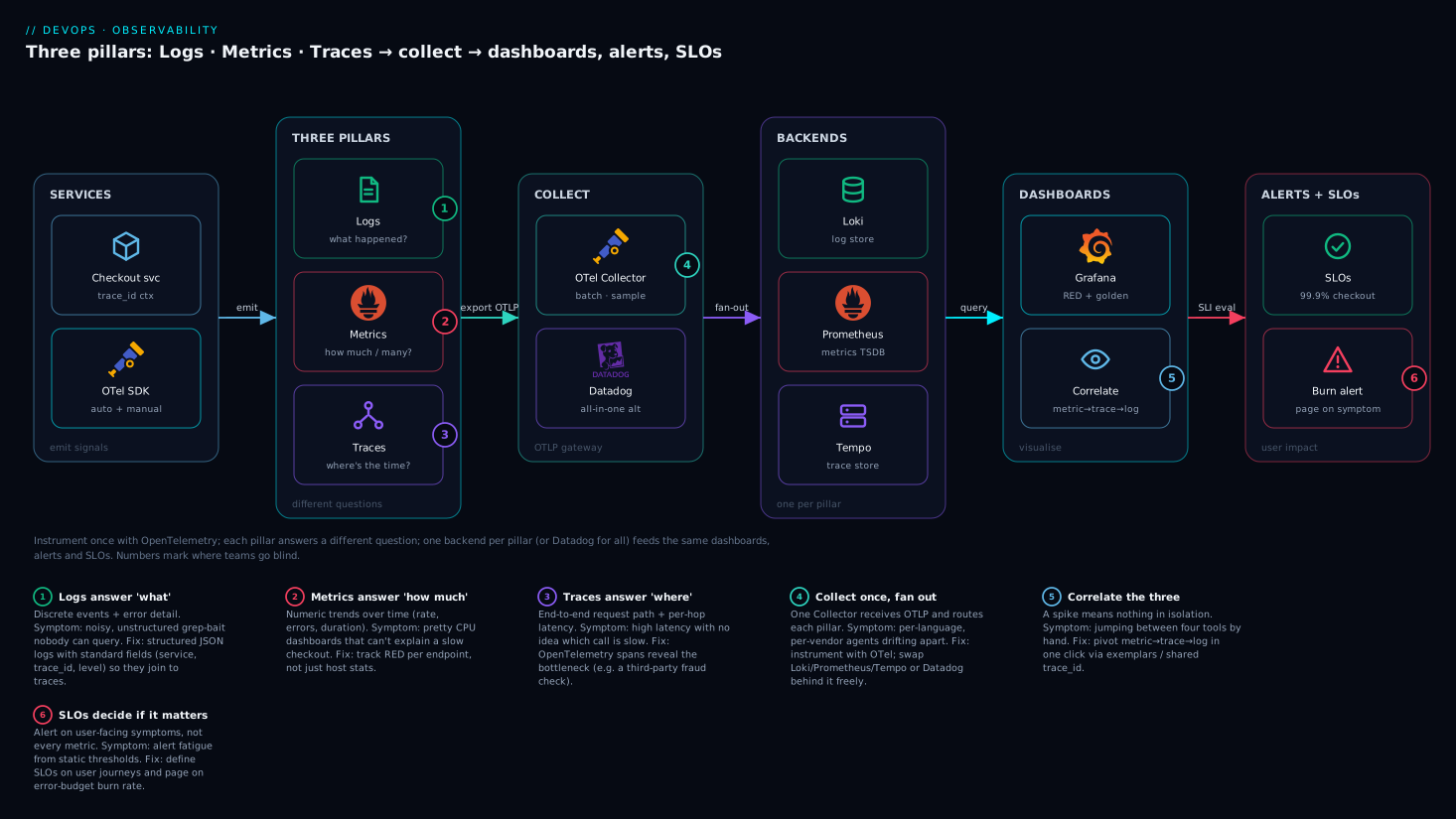
The system reads left to right, from the code that emits signals to the humans who get paged. Your instrumented services (each carrying the OpenTelemetry SDK) emit all three pillars over OTLP to an OpenTelemetry Collector, which is the single chokepoint where you batch, redact PII, and tail-sample. From there the Collector fans out by signal: metrics flow to Prometheus (scraped or remote-written), traces to Tempo, and logs to Loki. Sitting above all three, Grafana is the single query surface — it reads metrics, traces, and logs, and stitches them together so an exemplar on a latency graph links to the trace, and the trace links to the logs. Prometheus also feeds Alertmanager, which evaluates the SLO burn-rate rules: when checkout is burning its error budget too fast, Alertmanager routes a page (deduplicated and grouped) to on-call. The whole left-to-right flow is one pipeline: emit → collect → store-by-signal → visualize-and-correlate → alert-on-budget → page.
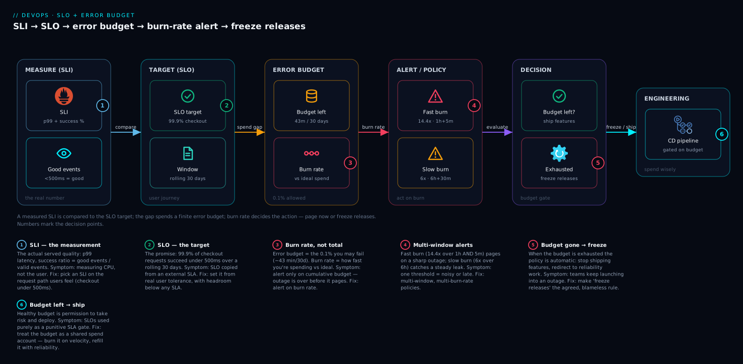
The second diagram is the reliability loop that decides when that page fires. An SLI (the measured good-events ratio) is compared against the SLO (the target); the gap is the error budget; the rate at which you consume that budget is the burn rate; and a burn rate above the multi-window thresholds triggers the alert. Read it as a feedback loop: a healthy SLI keeps the budget full and the alert quiet and lets you ship; a degrading SLI drains the budget, drives the burn rate up, and — once it crosses the fast-burn threshold — pages someone before users notice at scale.
Real-world scenario
Meridian Commerce runs a 28-service e-commerce platform on Kubernetes — about 9,000 requests/second at peak, 14 engineers across four squads, all on a self-hosted Grafana/Prometheus/Loki/Tempo stack. Their observability was the classic “metrics and dashboards” trap: 60-odd Grafana dashboards, alerts that fired on pod CPU and memory, and unstructured logs in Loki with pod as a label (which had quietly created 400,000 active streams and was costing them a fortune in object storage). On-call received roughly 40 pages a week; by the squads’ own admission, they muted most of them.
The breaking incident: a Black Friday dry-run at 2× normal load. Checkout p95 climbed from 280 ms to 4.2 seconds and the error rate hit 6%. The CPU-based alerts stayed green — no pod was saturated, because the latency was external wait, not compute. So no page fired until a customer-support escalation 25 minutes in. The on-call engineer opened eight dashboards, could not localize it, and spent 50 minutes before manually pulling a single trace (they had tracing, but at 100% head sampling it was so expensive they had quietly capped it at 1%, and the slow requests were mostly not in the 1%). The culprit, once found: the recommendations service made a synchronous call to a personalization API with no timeout, and under load that API’s p99 blew out to 6 seconds — every checkout waited on it. Total time to resolution: 90 minutes.
The rebuild took six weeks and was almost entirely removing and refocusing, not adding. They migrated to OpenTelemetry across all 28 services (auto-instrumentation got them 80% for free; manual spans covered the domain calls like the personalization fetch). They put an OTel Collector in front of every node, moved sampling there as tail sampling (keep 100% of errors and everything over 500 ms, 5% of the rest), and dropped trace cost by 70% while capturing every slow request. They fixed Loki cardinality by dropping the pod label and templatizing URLs — 400,000 streams fell to 11,000, and the storage bill dropped by two-thirds. They defined SLOs from three user journeys (checkout, search, login) instead of from infrastructure, and replaced 40 CPU/memory alerts with 12 multi-window burn-rate alerts — one fast-burn page and one slow-burn ticket per journey.
The payoff showed at the next load test. Checkout latency degraded the same way (the personalization API was still fragile) — but this time the fast-burn alert paged in 4 minutes, the on-call clicked the exemplar on the checkout latency panel straight into a slow trace, saw the 6-second personalization span lit red, and shipped a timeout-plus-fallback in 20 minutes. MTTD went from 25 minutes to 4; MTTR from 90 minutes to 24. Pages per week fell from ~40 to ~6, and — the cultural win — on-call stopped muting them, because every page now corresponded to real user pain. The lesson on their wiki: “We didn’t need more telemetry. We needed to alert on the three numbers users feel, and to make every page worth waking up for.”
The before/after, because the contrast is the whole argument:
| Dimension | Before (metrics + dashboards) | After (OTel + SLOs + burn-rate) |
|---|---|---|
| Alerting basis | Pod CPU/memory thresholds | Multi-window burn rate on 3 journeys |
| Pages / week | ~40 (mostly muted) | ~6 (all actioned) |
| MTTD (checkout incident) | 25 min (support escalation) | 4 min (fast-burn page) |
| MTTR | 90 min | 24 min |
| Trace coverage of slow requests | ~1% (head-sampled, capped for cost) | ~100% (tail-sampled on latency) |
| Loki active streams | ~400,000 | ~11,000 |
| Monthly observability spend | High & rising | Down ~55% |
Advantages and disadvantages
Full three-pillar observability with SLOs is the right model for any non-trivial distributed system — but it is an investment with real downsides if done carelessly. Weigh it honestly:
| Advantages | Disadvantages |
|---|---|
| You can ask new questions of production without shipping code | Instrumentation is real engineering effort across every service |
| Alerts fire on user pain (SLOs), not proxies (CPU) → less noise, faster detection | SLOs require deciding what “good” means — a cross-team negotiation |
| Metric → trace → log correlation collapses MTTR | Correlation only works if you standardized IDs (OTel) up front |
| OpenTelemetry means no backend lock-in — swap vendors freely | OTel has a learning curve; the spec moves fast |
| Error budgets turn reliability into a shared, data-driven decision | Budgets can be gamed or ignored without org buy-in |
| Tail sampling keeps every anomaly at a fraction of the cost | Tail sampling needs Collector infra and memory headroom |
| Open-source stack (Prom/Loki/Tempo/Grafana) is free of license cost | Self-hosting is operational toil; someone runs the runners |
The model pays off most for microservice platforms, high-traffic consumer apps, and multi-tenant SaaS — anywhere failures are emergent and per-request detail matters. It is over-engineering for a single monolith with light traffic, where a good APM agent and structured logs suffice. The downsides are all manageable: the instrumentation effort is front-loaded and then amortized; the SLO negotiation is a one-time exercise per journey; the cost levers (cardinality, sampling) are exactly what the rest of this article taught you to pull. The failure mode is doing the expensive half (collect everything) without the valuable half (SLOs, correlation, cost control) — which is how Meridian started.
Hands-on lab
Stand up the full open-source stack locally with Docker Compose, instrument a tiny service with OpenTelemetry, generate traffic, and watch a metric → trace → log correlation — then a burn-rate alert. Everything here runs free on a laptop; teardown is one command.
Step 1 — Project layout and the Compose file. Create a working directory and the stack:
mkdir obs-lab && cd obs-lab
# docker-compose.yaml — Prometheus, Tempo, Loki, Grafana, OTel Collector
services:
  prometheus:
    image: prom/prometheus:v2.54.1
    command: ["--config.file=/etc/prometheus/prometheus.yml", "--enable-feature=exemplar-storage"]
    volumes: ["./prometheus.yml:/etc/prometheus/prometheus.yml"]
    ports: ["9090:9090"]
  tempo:
    image: grafana/tempo:2.6.0
    command: ["-config.file=/etc/tempo.yaml"]
    volumes: ["./tempo.yaml:/etc/tempo.yaml"]
    ports: ["3200:3200"]
  loki:
    image: grafana/loki:3.2.0
    command: ["-config.file=/etc/loki/local-config.yaml"]
    ports: ["3100:3100"]
  otel-collector:
    image: otel/opentelemetry-collector-contrib:0.110.0
    command: ["--config=/etc/otel-collector.yaml"]
    volumes: ["./otel-collector.yaml:/etc/otel-collector.yaml"]
    ports: ["4317:4317", "4318:4318", "8889:8889"]
  grafana:
    image: grafana/grafana:11.2.0
    environment: ["GF_AUTH_ANONYMOUS_ENABLED=true", "GF_AUTH_ANONYMOUS_ORG_ROLE=Admin"]
    ports: ["3000:3000"]
Step 2 — Prometheus config that scrapes the Collector’s metrics endpoint.
# prometheus.yml
global: { scrape_interval: 5s }
scrape_configs:
  - job_name: otel-collector
    static_configs: [{ targets: ["otel-collector:8889"] }]
Step 3 — The OTel Collector config (OTLP in; metrics to Prometheus-scrape, traces to Tempo, logs to Loki). Reuse the Collector config from the OpenTelemetry section above, pointing otlphttp/tempo at http://tempo:4318 and otlphttp/loki at http://loki:3100/otlp.
Step 4 — Start the stack and verify.
docker compose up -d
docker compose ps          # all 5 services should be "running"
curl -s localhost:9090/-/healthy && echo "prometheus ok"
curl -s localhost:3000/api/health | grep -q ok && echo "grafana ok"
Expected: five running containers; both health checks print ok.
Step 5 — A tiny instrumented service. Write a Flask app with a histogram, a counter, and a manual span that occasionally errors and is occasionally slow:
# app.py
import random, time
from flask import Flask
from opentelemetry import trace
app = Flask(__name__)
tracer = trace.get_tracer("checkout")

@app.route("/checkout")
def checkout():
    with tracer.start_as_current_span("checkout.process") as span:
        span.set_attribute("route", "/checkout")
        # 10% slow (simulate the fraud-check bottleneck), 5% error
        if random.random() < 0.10:
            time.sleep(0.8)                       # > 500ms SLO boundary
            span.set_attribute("slow", True)
        if random.random() < 0.05:
            span.set_status(trace.StatusCode.ERROR, "payment failed")
            return "error", 500
        return "ok", 200
pip install flask opentelemetry-distro opentelemetry-exporter-otlp
opentelemetry-bootstrap -a install
OTEL_SERVICE_NAME=checkout OTEL_EXPORTER_OTLP_ENDPOINT=http://localhost:4318 \
OTEL_METRICS_EXPORTER=otlp OTEL_TRACES_EXPORTER=otlp \
  opentelemetry-instrument flask run -p 8000
Step 6 — Generate traffic.
# 2000 requests; ~10% will be slow, ~5% will 500
for i in $(seq 1 2000); do curl -s localhost:8000/checkout >/dev/null; done
echo "traffic done"
Step 7 — See the metric, then the trace, then the log (the correlation pivot). In Grafana (localhost:3000), add Prometheus, Tempo, and Loki datasources (all by their container DNS names), then:
- Explore Prometheus:
histogram_quantile(0.95, sum(rate(http_server_duration_milliseconds_bucket[1m])) by (le))— you’ll see p95 spike from the 10% slow requests. - Click an exemplar dot on that graph → it opens the slow trace in Tempo, showing the 0.8 s
checkout.processspan. - From the errored span, pivot to Loki filtered by
trace_idto read the failure context.
Step 8 — A burn-rate alert. Add the recording rule and the fast-burn alert from the burn-rate section (route /checkout, SLO 99.9%) to prometheus.yml under rule_files, reload Prometheus (curl -X POST localhost:9090/-/reload), and confirm in Status → Rules that CheckoutErrorBudgetFastBurn is loaded and evaluating. With a 5% error rate against a 0.1% budget, it will be firing — exactly as designed.
Step 9 — Validation checklist.
| Check | Command / action | Expected |
|---|---|---|
| Metrics flowing | Prometheus → http_server_duration_milliseconds_count |
Non-zero, climbing |
| p95 reflects slow path | The histogram_quantile query | Spikes toward ~800 ms |
| Traces captured | Tempo search in Grafana | Slow + errored traces present |
| Exemplars clickable | Latency panel dots | Link to a real trace |
| Logs joinable | Loki by trace_id |
Returns the matching lines |
| Burn-rate alert | Prometheus → Alerts | CheckoutErrorBudgetFastBurn firing |
Step 10 — Teardown.
docker compose down -v # stops and removes containers + volumes
Common mistakes & troubleshooting
The failure modes that bite real teams — symptom, root cause, how to confirm, and the fix:
| # | Symptom | Root cause | Confirm with | Fix |
|---|---|---|---|---|
| 1 | Prometheus OOMs / queries time out | Cardinality explosion — an unbounded label (user_id, raw URL) | topk(10, count by (__name__)({__name__=~".+"})) |
labeldrop / templatize the path; recording rules |
| 2 | Traces stop at a service boundary | Context not propagated across a hand-rolled client / queue | Trace waterfall ends abruptly; child trace has new trace_id |
Inject/extract traceparent; use OTel auto-instrumentation |
| 3 | You never have a trace of the slow request | Head sampling dropped it (random 1%) | Slow requests rarely in Tempo | Switch to tail sampling on latency + errors |
| 4 | Pager fires constantly on noise | Static thresholds on CPU/memory, no SLO | Alerts unrelated to user impact | Replace with multi-window burn-rate SLO alerts |
| 5 | Site is broken but no alert fired | Alerting on a proxy (CPU) not the symptom (latency/errors) | CPU green during a latency incident | SLI from latency/errors; alert on burn rate |
| 6 | p99 looks fine, users complain | Using a summary (un-aggregatable) or only the average | Averaged quantiles across pods are meaningless | Use histograms; compute histogram_quantile |
| 7 | Loki bill is huge | High-cardinality labels (pod, trace_id) on streams | logcli series shows millions of streams |
Keep labels low-card; put IDs in the log body |
| 8 | Logs can’t be tied to a trace | No trace_id in log lines |
Logs have no correlation field | Inject trace context into the logger |
| 9 | Burn-rate alert won’t clear after incident | Single long window keeps firing for an hour | Alert lingers post-recovery | Add the short window (multi-window pattern) |
| 10 | Health-check-style SLI flaps | SLI measured at the LB, not from real user requests | SLI uncorrelated with real traffic | Measure SLI from actual request telemetry |
| 11 | Collector drops spans under load | No memory_limiter / batch; backend backpressure |
Collector logs “refused”/queue full | Add memory_limiter + batch; scale Collector |
| 12 | Two services report different p99 for the same call | Each computed quantiles client-side (summary) | Numbers don’t reconcile | Histograms + server-side aggregation |
| 13 | Datadog/Prometheus cost jumped after a deploy | New label or a custom metric per request | Diff active series before/after | Audit the new metric; drop/templatize the label |
| 14 | “Unknown service” all over traces | service.name resource attribute unset |
Tempo shows unknown_service |
Set OTEL_SERVICE_NAME / resource attributes |
The pivot order in an incident is reliable: to learn whether something is wrong and how bad, reach for metrics (RED plus SLO burn), then pivot to a trace for one slow/failed example. To learn where the latency is, reach for traces (the waterfall), then pivot to logs for the failing span’s context. To learn what exactly failed on this request, reach for logs (filtered by trace_id), then pivot back to the trace for the upstream cause. To learn whether it’s us or a dependency, read the trace (which span is slow) and jump to that dependency’s own dashboard. And to learn whether a resource is saturated, reach for metrics (USE), then logs for OOM/eviction events.
Best practices
- Instrument with OpenTelemetry, export through a Collector. One instrumentation, any backend; the Collector is where you batch, redact, and sample without redeploying apps.
- Structure every log line as JSON/logfmt with stable field names and a
trace_id. If you would log it on every request, make it a metric instead. - Treat labels as a budget. A label must be bounded and something you
group by. User IDs, request IDs, and raw URLs go in logs and traces, never metric labels. - Use histograms for latency, with buckets straddling your SLO boundary. Never average percentiles; never use summaries you need to aggregate.
- Define SLOs from user journeys, not infrastructure. Checkout, search, login — the things users do — not CPU or pod count.
- Alert on multi-window burn rate, not static thresholds. Fast burn pages; slow burn tickets; require a short and a long window so blips don’t page and alerts clear fast.
- Set SLOs stricter than SLAs, and tie the error budget to a release policy: healthy budget → ship; exhausted budget → freeze and stabilize.
- Tail-sample traces: keep 100% of errors and everything over your latency threshold, sample the boring successes. You get every anomaly at a fraction of the cost.
- Make correlation one click. Exemplars on latency graphs → traces → logs by
trace_id. If you can’t pivot, you don’t have observability, you have three firehoses. - Annotate deploys on dashboards so “the spike began at 14:02” is visible, not inferred. Most incidents are a recent change.
- Build dashboards RED-on-top, USE-below, one per service, with template variables — symptoms then causes, navigable by ownership.
- Review cardinality and cost monthly. Diff active series after every deploy; a single new label can quietly double the bill.
Security notes
Observability data is some of the most sensitive data you hold — it is a high-fidelity record of what your system did, often including who did it. Treat it accordingly:
| Concern | Risk | Control |
|---|---|---|
| PII / secrets in telemetry | Emails, tokens, card numbers in logs/spans = plaintext breach | Redact at source; scrub in the Collector (attributes processor delete); never log secrets |
| Telemetry as an attack-surface | An exposed Prometheus/Grafana leaks topology & data | Auth on every UI; network-isolate scrape & OTLP endpoints |
| OTLP in transit | Spans/logs sniffed on the wire | TLS on OTLP (gRPC/HTTP); mTLS Collector↔backend |
| Access control | Anyone can read anyone’s logs/traces | RBAC in Grafana; per-tenant isolation in Loki/Mimir/Tempo |
| Retention & compliance | Holding PII-laden logs too long breaches GDPR/PCI | Short hot retention; scrub before storage; data-residency-aware backends |
| Cardinality as DoS | An attacker (or bug) floods unbounded labels → backend down | Enforce label limits; relabel-drop aggressively; rate-limit ingestion |
| Audit integrity | Logs used for audit can be tampered/lost | Ship off-box immediately; immutable/append-only audit stores |
Two rules above all: redact PII at the source and again in the Collector (defense in depth — never rely on a single scrubbing layer), and authenticate and network-isolate every observability endpoint — an open Grafana or Prometheus is a map of your entire system handed to an attacker. For the alerting side, integrate on-call securely as covered in incident response, on-call, PagerDuty alert routing and runbooks.
Cost & sizing
Observability famously costs 10–30% of infrastructure spend when it runs away, and the two levers you already learned — cardinality and sampling — are 80% of cost control. What drives the bill, and how to size each:
| Cost driver | What inflates it | How to control | Rough magnitude |
|---|---|---|---|
| Metric series (Prometheus/Datadog) | Cardinality — every label combination | Relabel-drop, templatize URLs, recording rules | Datadog ~₹15–40 / 100 custom metrics/mo; self-host = storage + RAM |
| Log volume (Loki/Datadog) | Bytes ingested; high-card stream labels | Sample info logs; low-card labels; short hot retention | Datadog logs ~₹8–12 / GB ingested; Loki ≈ object-storage cost |
| Trace spans (Tempo/Datadog APM) | Sampling rate × spans/request × retention | Tail-sample; cap retention to days | Datadog APM per-host + per-span; Tempo ≈ object storage |
| Self-hosting compute | Running Prom/Loki/Tempo/Grafana + Collectors | Right-size; downsample old metrics | A few medium VMs / a node pool |
| Retention | Keeping everything hot for months | Hot days → cold weeks → drop | Cold/object storage is ~10× cheaper than hot |
Sizing rules of thumb that keep you out of trouble: a well-sized Prometheus node is comfortable to about 1–2 million active series (beyond that, shard or move to Mimir); keep under ~6–8 bounded labels per metric and audit anything above; tail-sample traces to retain ~100% of errors and slow requests plus 1–10% of the rest; hold logs 7–14 days hot, with longer cold retention only if compliance demands it; and give latency histograms 8–12 buckets straddling your SLO boundary — every extra bucket is another series.
The open-source stack has no license cost but real operational cost (you run the runners, you carry the upgrade toil). Datadog and peers flip that: high license cost, near-zero ops. The crossover is usually team size and scale — a small team often comes out ahead on a managed/SaaS backend (Grafana Cloud, Datadog) because the engineer-hours to self-host exceed the license; a large platform team with scale economics self-hosts. The honest comparison:
| Dimension | Open-source (Prom/Loki/Tempo/Grafana) | Datadog (and peers) |
|---|---|---|
| License cost | None | High, usage-metered (hosts, metrics, GB, spans) |
| Operational effort | You run & upgrade everything | Near-zero — fully managed |
| Time to value | Days–weeks to wire up | Hours (agent + UI) |
| Correlation UX | Good (Grafana exemplars) — you configure it | Excellent, out of the box |
| Lock-in | None (especially via OTel) | Real — but OTel ingestion mitigates it |
| Best for | Large teams; cost-at-scale sensitive | Small/medium teams; speed over license cost |
The cost-governance deep dives — Prometheus cardinality control and cost governance, Loki LogQL cardinality and chunk storage tuning, and the trade-offs of a Datadog single pane for multi-cloud operations — go far deeper on each lever.
Interview & exam questions
Q1. What is the difference between monitoring and observability? Monitoring answers predefined questions (“is CPU > 80%?”) via known dashboards and alerts. Observability is the property that lets you ask new, unanticipated questions of production from the telemetry you already emit — without shipping code. You build it by emitting logs, metrics, and traces that share identifiers and can be correlated.
Q2. Why can’t logs replace metrics, or metrics replace traces? Each is a different data shape for a different question. Logs are per-event and rich but expensive and slow to aggregate (“how often” is costly). Metrics aggregate cheaply but can’t explain why a number moved or show one request’s detail. Traces show cross-service latency breakdown that neither can. You need all three because no two cover the third’s strength.
Q3. What is metric cardinality and why does it matter? Cardinality is the number of unique time series — the product of every label’s distinct values. It is the primary driver of metrics cost and query latency. A single unbounded label (user_id, raw URL) can create millions of series and crash Prometheus. Labels must be bounded dimensions you group by; identifiers belong in logs/traces.
Q4. Head vs tail sampling — when would you use each? Head sampling decides at request start (cheap, but blind to outcome — may drop the error you needed). Tail sampling buffers the whole trace and decides after seeing the result (keep all errors and slow requests, sample the rest) — far better signal at the cost of Collector buffering. Use head to bound the firehose, tail to guarantee you keep anomalies.
Q5. Define SLI, SLO, error budget, and SLA. An SLI is a measured ratio of good events to valid events (e.g. % of requests fast and successful). An SLO is a target for that SLI over a window (99.9%/28d). The error budget is 100% − SLO — the allowed badness. An SLA is a contractual promise with penalties; you set your SLO stricter than your SLA to react before breaching.
Q6. What is an error budget and how does it change how teams ship? It’s the inverse of the SLO — the failures you’re permitted. It reframes reliability from “never fail” to “spend a finite budget deliberately.” Healthy budget → ship boldly, take risks; exhausted budget → freeze features and stabilize. It’s a shared currency between devs (speed) and SREs (stability).
Q7. Why is burn-rate alerting better than static thresholds? Static thresholds fire on momentary blips (noise → fatigue) and with no sense of urgency (same alert whether you have hours or seconds of budget). Burn-rate alerts fire on how fast you’re consuming the error budget, over multiple windows — fast burn pages immediately, slow burn tickets — so alerts correlate with real urgency and clear quickly.
Q8. What is a burn rate of 14.4 over a 30-day SLO? Burn rate is budget-consumed-per-time normalized so 1.0 = on pace to exhaust exactly at the window’s end. 14.4 means you’re spending 14.4× too fast — you’d burn a 30-day budget in about 2 days. It’s the standard fast-burn paging threshold (with a 1h long + 5m short window).
Q9. What is OpenTelemetry and why does it matter? OTel is the CNCF vendor-neutral standard — APIs, SDKs, semantic conventions, and the OTLP protocol — for logs, metrics, and traces. You instrument once and export anywhere (Prometheus, Tempo, Datadog, etc.) by changing an exporter, not your code. It ends backend lock-in and is the foundation for cross-pillar correlation.
Q10. What breaks a distributed trace and how do you prevent it? A trace breaks when context isn’t propagated across a hop — the downstream service starts a new trace_id instead of continuing the parent’s. Prevent it by propagating the W3C traceparent header (inject upstream, extract downstream); OTel auto-instrumentation handles common frameworks, but async/queue boundaries and hand-rolled clients need manual propagation.
Q11. RED vs USE — what are they and when do you use each? RED (Rate, Errors, Duration) describes request-driven services — what users feel. USE (Utilization, Saturation, Errors) describes resources — what the system feels. A good dashboard puts RED on top (symptoms) and USE below (causes), so incidents read “errors up → because the pool is saturated.”
Q12. Why use a histogram instead of a summary for latency? A histogram bucketizes observations so percentiles are computed server-side and can be aggregated across instances (histogram_quantile). A summary computes quantiles client-side and cannot be aggregated — averaging two services’ p99s is mathematically meaningless. For anything you’ll aggregate, use histograms.
These map directly to the SRE/DevOps portions of certifications and interviews: the Prometheus Certified Associate (PCA), the Kubernetes and Cloud Native Associate (KCNA) observability domain, and SRE interview loops at most platform-heavy companies.
Quick check
- You add a
customer_emaillabel to a Prometheus counter and your bill triples. What happened, and what’s the fix? - Checkout p99 is fine but support says the site is slow. Name two likely measurement mistakes.
- Your fast-burn SLO alert keeps firing for an hour after the incident cleared. What’s missing from the rule?
- You’re at 100% head sampling and can never find a trace of the slow request. What change fixes both cost and signal?
- An SLO of 99.9% over 30 days — roughly how much “bad” time does that permit?
Answers
- Cardinality explosion —
customer_emailis unbounded, creating one series per customer. Fix:labeldropit (emails belong in logs/traces, not metric labels), and audit for other unbounded labels. - Either you’re looking at the average (which hides the tail), or you’re using a summary and averaging quantiles across pods (meaningless). Use histograms and
histogram_quantileaggregated server-side. Also possible: the SLI is measured at the load balancer, not from real user requests. - The short window. The multi-window pattern requires both a long (1h) and a short (5m) window to fire; the short window makes the alert resolve quickly once the burn stops, instead of lingering for the full long window.
- Switch to tail sampling in the Collector — keep 100% of errors and everything over your latency threshold, sample the boring successes. You capture every slow request and cut volume sharply.
- About 43.8 minutes per 30 days (0.1% of the window). Memorize the nines table: 99% ≈ 7.3h, 99.9% ≈ 44m, 99.99% ≈ 4.4m per 30 days.
Glossary
| Term | Definition |
|---|---|
| Observability | The property of a system that lets you ask new questions of production from emitted telemetry, without shipping code. |
| Three pillars | Logs, metrics, and traces — the three complementary signal types. |
| Metric | A numeric value sampled over time, tagged with a small set of labels. |
| Cardinality | The number of unique time series; the product of every label’s distinct values. The main cost/perf driver. |
| Histogram | A metric type that bucketizes observations so percentiles can be computed and aggregated server-side. |
| Trace | A tree of timed spans representing one request’s journey across services. |
| Span | One timed operation within a trace, with attributes, a parent, and a status. |
| Context propagation | Passing trace context (e.g. the W3C traceparent header) across service hops so spans join one trace. |
| OpenTelemetry (OTel) | The CNCF vendor-neutral standard (API, SDK, semantic conventions, OTLP) for all three signals. |
| OTLP | OpenTelemetry’s wire protocol for transporting telemetry. |
| Collector | The OTel agent that receives, processes (batch/redact/sample), and exports telemetry. |
| Sampling | Keeping a representative or interesting subset of traces to control volume. |
| Head / tail sampling | Deciding at request start (head) vs after the trace completes (tail). |
| SLI | Service Level Indicator — a measured ratio of good events to valid events. |
| SLO | Service Level Objective — a target for an SLI over a window. |
| Error budget | 100% − SLO; the amount of unreliability you’re permitted. |
| Burn rate | The speed of consuming the error budget; 1.0 = on pace to exhaust at window’s end. |
| SLA | Service Level Agreement — a contractual reliability promise with penalties. |
| RED / USE | Rate-Errors-Duration (request-centric) / Utilization-Saturation-Errors (resource-centric) metric recipes. |
| Exemplar | A sample trace_id attached to a histogram bucket, enabling the metric → trace pivot. |
| Golden signals | Latency, errors, traffic, saturation — the four user-facing health signals. |
Next steps
- Go deep on the foundations in Monitoring and observability basics: logs, metrics, traces, then control the metrics cost lever in Prometheus cardinality control with relabeling and cost governance.
- Master the reliability layer in SLO error budgets with multi-window burn-rate alerting and tame the pager with Alertmanager routing trees, inhibition and deduplication.
- Build the tracing pipeline in distributed tracing with Tempo, Jaeger, exemplars and correlation and scale it with OpenTelemetry Collector tail-based sampling and load balancing.
- Connect observability to delivery: feed these signals into deployment strategies: blue-green, canary, rolling and measure your delivery health with DORA metrics and platform engineering.
- Weigh the build-vs-buy decision with Datadog as a single pane for multi-cloud operations and engineer your dashboards with Grafana dashboard engineering: RED, USE and variables.