In a nutshell
“Make it faster” sounds like a coding problem — find the slow function, rewrite it, ship. On Google Cloud, performance optimization is something broader and more disciplined: you engineer the whole system so it meets a stated speed target under real load, and you keep it there as traffic grows and Google’s own services evolve. Performance is a measured number on a dashboard, not a gut feeling — and the pillar’s first commandment is that you cannot optimize what you have not first defined and measured.
The mental model that makes it click: run your system like a restaurant kitchen during the Saturday dinner rush. The menu promises every dish in twelve minutes; the kitchen’s whole job is to keep that promise whether ten covers walk in or four hundred. Six moves make that possible, and a well-run kitchen makes all six by design:
- Print the promise on the menu. “Twelve minutes or it’s on us” is a number the whole kitchen is judged against — performance requirements and SLOs (p50/p95/p99 latency, throughput, concurrency), written down before anyone tunes a thing.
- Staff the right stations, not just more bodies. A grill order needs a grill cook, not three extra salad hands — right-sizing and right-shaping compute, storage, and databases to the actual bottleneck (a compute-optimized C3 for CPU-bound work, an M-series for memory-bound, a Hyperdisk that buys IOPS without buying terabytes).
- Call in staff for the rush, send them home at close. Scale the line up when tickets pile in and down to a skeleton crew at midnight — autoscaling to demand rather than paying for a peak brigade 24×7.
- Seat guests across the room, spill to the annex when full. A host who packs one section while another sits empty sinks the service — global load balancing routes each request to the nearest healthy backend and spills a saturated region to the next.
- Prep the mise en place before the doors open. The fastest dish is the one already plated — caching at every tier (Cloud CDN at the edge, Memorystore in memory, read replicas at the database) so the hottest requests never reach the kitchen at all.
- Put an expediter on the pass. Someone watches every ticket’s clock, spots the station falling behind, and re-times the line — continuous monitoring, tracing, and profiling (Cloud Trace finds the slow hop, Cloud Profiler finds the hot function) that turns “it feels slow” into “the entitlement call is 380 ms of the 500.”
This lesson is the Performance Optimization pillar of the Google Cloud Architecture Framework, and it teaches all six moves as architecture: the performance principles, right-sizing resource selection, autoscaling to the demand curve, global load balancing, multi-tier caching, and the monitoring-driven tuning loop that keeps it all honest. The through-line the whole pillar insists on is the perf-versus-cost trade-off: performance is never free — every “9” of latency you shave costs money, an error budget, or both — so the goal is not “as fast as possible” but “fast enough to meet the target, provably, at the lowest sustainable cost.” That is why this pillar sits last, applied to a system the other five pillars already shaped.
Level: Advanced · Time: ~48 min
Prerequisites. You should be comfortable with how you chose your services in the System Design pillar (Cloud Run vs GKE vs Spanner, and why), because Performance Optimization tunes within those choices rather than re-making them. You should know what an SLO and error budget are from the Reliability pillar — a latency SLO is your performance gate — and you should have read the Cost Optimization pillar, because every performance lever here has a cost sign you must weigh. To go deeper on the measurement layer, the Cloud Monitoring & Operations Suite deep dive covers the dashboards, SLOs, Trace, and Profiler this pillar leans on. If any of those are unfamiliar, skim them first — this lesson assembles them into a performance-engineering discipline.
After this lesson you will be able to:
- Turn a vague “make it fast” into a performance requirements specification — per-service p50/p95/p99 latency, throughput, and concurrency — and express it as a Cloud Monitoring latency SLO with a burn-rate alert.
- Decompose a p99 latency budget across the critical path, find the hop that blows it with Cloud Trace, and choose the right lever (right-size, cache, replica, async) to fix it.
- Right-size and right-shape compute (machine family, custom types, Cloud Run concurrency), storage (Hyperdisk IOPS/throughput), and databases (replicas, slots, BI Engine) from telemetry rather than guesses.
- Build an elastic scaling path that holds latency through a ramp — scaling on the right signal (concurrency, Pub/Sub backlog), killing cold starts with
min-instances, and validating it with a load/spike test. - Design multi-tier caching (edge, in-memory, DB read) with an explicit invalidation strategy (per-data-class TTLs, event-driven busts, versioned keys) and a hit-ratio alert.
- Stand up the continuous-tuning loop — Trace, always-on Profiler, SLO burn-rate alerts, load tests before peak — and make the perf-vs-cost trade-off explicit, tying every lever back to the other five pillars.
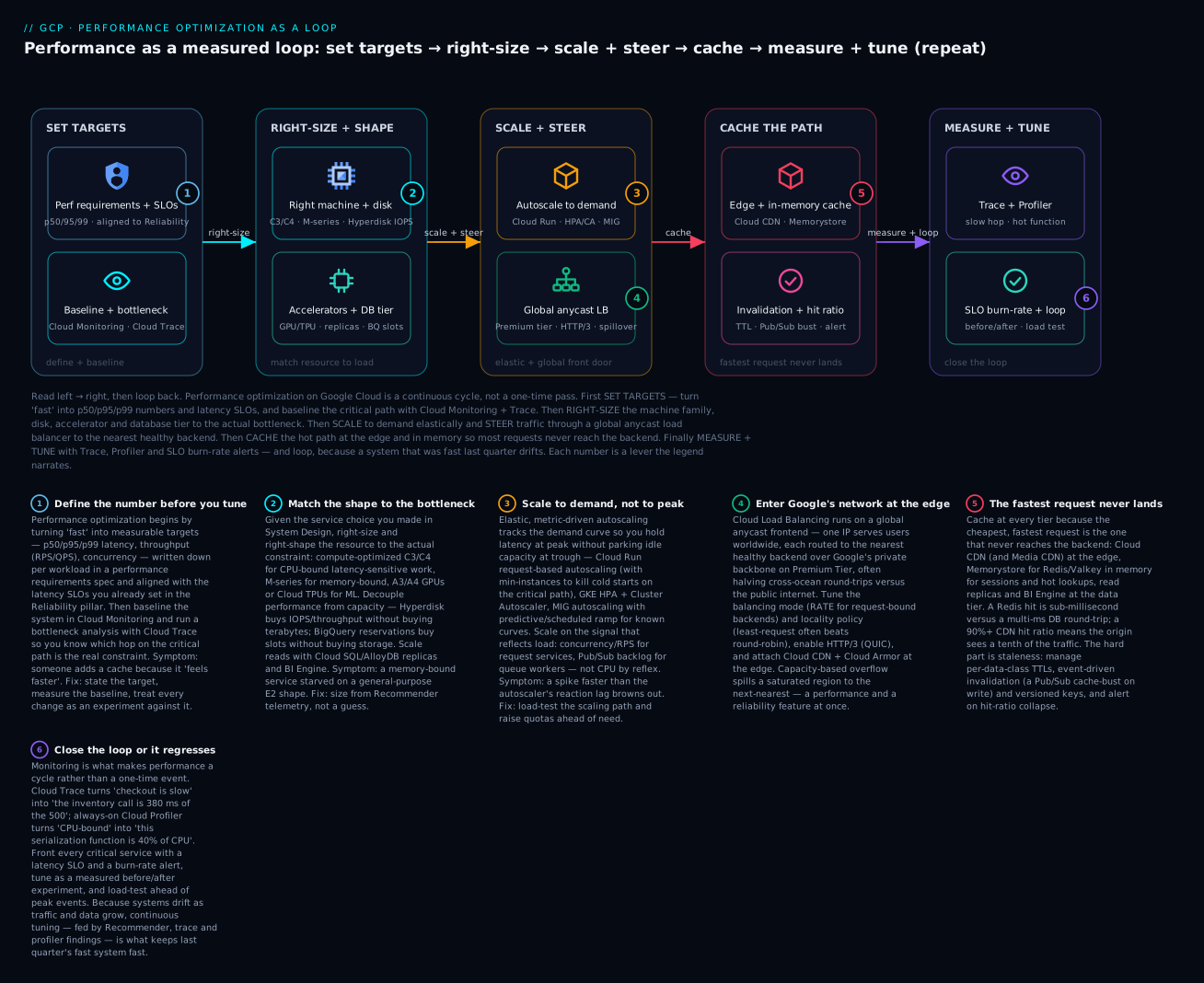
Read the diagram left → right, then loop back: you first set targets (turn “fast” into p50/p95/p99 numbers and latency SLOs, and baseline the critical path with Monitoring + Trace), then right-size the machine family, disk, accelerator, and database tier to the actual bottleneck, then scale to demand and steer traffic through a global anycast load balancer to the nearest healthy backend, then cache the hot path at the edge and in memory so most requests never reach the backend, and finally measure and tune with Trace, Profiler, and SLO burn-rate alerts — then loop, because a system that was fast last quarter drifts. The numbered badges are the levers the sections below unpack.
Where this fits
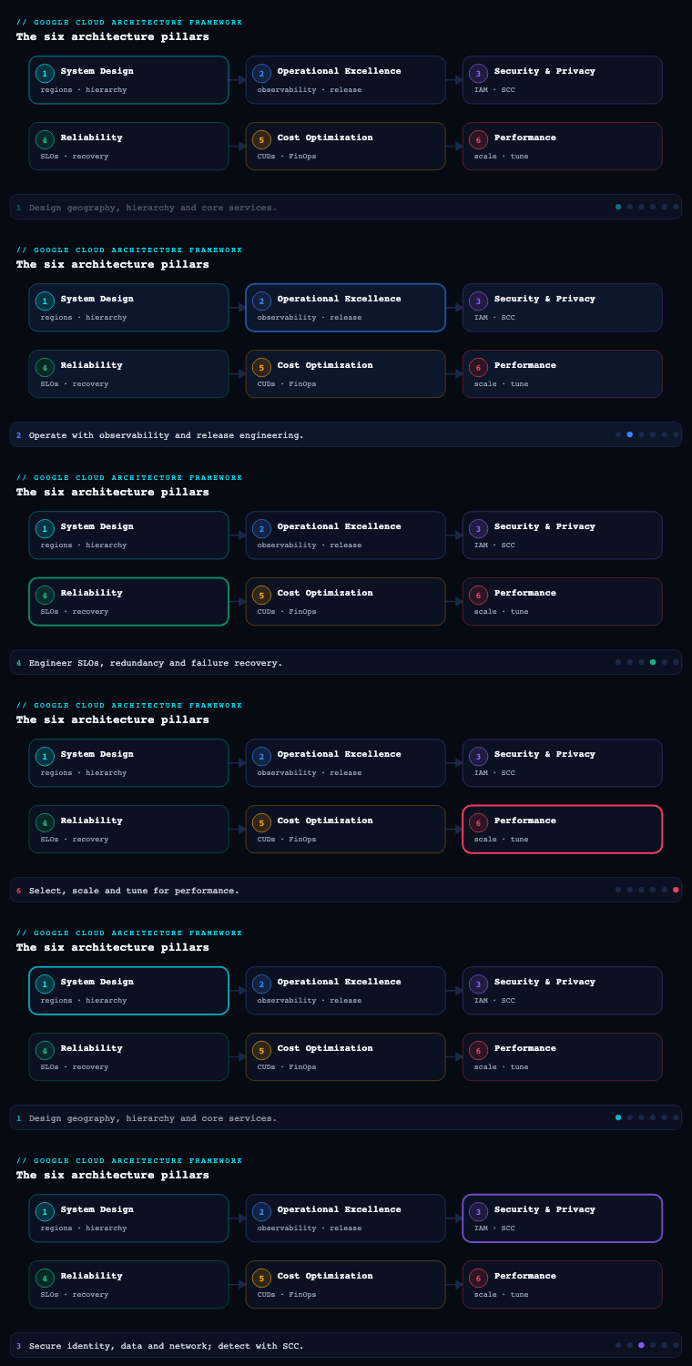
The Google Cloud Architecture Framework spans six pillars — System Design, Operational Excellence, Security, Privacy & Compliance, Reliability, Cost Optimization, and Performance Optimization — and Performance Optimization is part 6, the final pillar, deliberately placed last because it is the discipline that closes the loop: it takes the structural decisions from System Design, the SLOs and error budgets from Reliability, and the budgets and discounts from Cost Optimization, and asks the empirical question they all defer — does the system actually meet its latency, throughput, and efficiency targets under real load, and how do we keep it there as traffic and Google’s own services evolve? Performance Optimization is not a one-time pass; it is a continuous cycle of setting performance requirements, selecting and right-sizing resources, scaling to demand, distributing load, caching aggressively, and then measuring and tuning — forever. It is where “well-architected” stops being a diagram and becomes a number on a dashboard.
Performance principles — the design philosophy for a fast, efficient system
Before you reach for an autoscaler or a CDN, the Architecture Framework asks you to internalize a small set of performance principles that govern how you optimize. They exist to stop two failure modes: optimizing the wrong thing (gut-feel tuning with no baseline), and optimizing in a way that quietly breaks reliability or cost.
The principles you are applying.
| Principle | What it means in practice | The consequence if you ignore it |
|---|---|---|
| Define performance requirements first | Turn “fast” into measurable targets — p50/p95/p99 latency, throughput (RPS/QPS), concurrency, time-to-first-byte — per workload | You tune blind; “good enough” is a moving opinion, not a gate |
| Take a data-driven, baseline-first approach | Measure before you change; every optimization is a hypothesis tested against a baseline | You ship “improvements” that regress p99 and never notice |
| Optimize incrementally and continuously | Performance work is iterative — one change, one measurement, one comparison | Big-bang tuning passes hide which change helped or hurt |
| Use elasticity, don’t over-provision | Scale to demand horizontally rather than buying for peak 24×7 | You pay for headroom you use 4 hours a month, or you fall over at peak |
| Design for the critical path | Optimize the user-facing latency path; push everything else off it (async, batch) | You speed up code no user waits on |
| Balance against the other pillars | Performance trades against cost, reliability, and sustainability — make the trade explicit | A faster system that blows the budget or the error budget is not well-architected |
| Identify and respect bottlenecks | The system is only as fast as its slowest resource on the path (CPU, memory, I/O, network, a downstream API) | You scale the tier that wasn’t the constraint |
Why it matters. Performance is the one pillar where intuition is most often wrong. The principle that does the most work is define requirements first, then baseline: without a stated p99 target and a measured starting point, “performance optimization” degenerates into someone adding a cache because it feels faster. The second highest-leverage principle is design for the critical path — most user-perceived latency lives in a handful of synchronous hops (an auth call, a database query, a downstream API), and the framework’s bias is to shorten that path (caching, read replicas, async offload) rather than micro-optimize code off it.
How to do it well. Make the requirements an artifact: a performance requirements specification that names, per service, the latency percentiles, throughput, and concurrency the workload must sustain, ideally aligned with the SLOs you already wrote in the Reliability pillar (latency SLOs and their error budgets are your performance gate). Establish a baseline with Cloud Monitoring dashboards and load tests before any tuning, and treat every change as a measured experiment. Record the bottleneck analysis — which resource is the constraint on the critical path — because that determines what you scale or cache. The principles map directly onto the sub-components that follow: requirements and bottlenecks feed resource selection, elasticity feeds scaling, critical-path thinking feeds load balancing and caching, and the whole loop closes in monitoring and continuous tuning.
Resource selection — right-sizing the compute, storage, and data primitives for performance
Resource selection in the Performance pillar is narrower and more empirical than the service-choice you made in System Design. There, you picked Cloud Run vs GKE vs Spanner by data model and operational fit. Here, you ask: given that choice, am I running the right machine shape, the right disk, the right tier, sized to the demand curve — and where is the performance actually limited?
The selection decisions you are actually making.
| Dimension | What you tune | GCP levers |
|---|---|---|
| Compute shape | CPU platform and machine family matched to the workload profile | Machine families: E2/N (general), C3/C4 (compute-optimized, latest Intel/AMD), M3/M4 (memory-optimized), A3/A4 + TPU (accelerator); Tau T2D/T2A for scale-out price/perf |
| Right-sizing | VCPU/memory matched to actual utilization, not guessed | Recommender rightsizing recommendations, VM Manager, custom machine types, Cloud Run CPU/memory + concurrency settings |
| Block storage performance | IOPS and throughput decoupled from capacity | Hyperdisk (Balanced / Extreme / Throughput) with independently provisioned IOPS & MB/s; Local SSD for ultra-low-latency scratch; regional PD when zone-survival matters |
| Object storage performance | Throughput and latency for data/AI pipelines | Cloud Storage with Anywhere Cache, Storage FUSE, Parallelstore, hierarchical namespace; right storage class + location |
| Database performance | Read scaling, query acceleration, in-memory engines | Cloud SQL read replicas, AlloyDB columnar engine + read pool, Spanner node/processing-unit sizing, Bigtable node count & SSD, BigQuery slots/reservations + BI Engine |
| Network performance | Path quality and tier | Premium vs Standard Network Service Tier, Cloud CDN, gVNIC, Tier_1 networking bandwidth, jumbo frames (MTU 8896) |
| Accelerators | GPU/TPU selection for ML/HPC | A3 (H100) / A4, Cloud TPU v5e/v5p/Trillium, GKE accelerator node pools, Dynamic Workload Scheduler |
Why it matters. The single most common performance defect in real estates is a mis-sized resource: a memory-bound service starved on a general-purpose E2 shape, a database VM throttled by a capacity-coupled disk, a BigQuery workload queuing on too few slots. Google’s modern primitives explicitly decouple the performance dimension from the capacity dimension — Hyperdisk lets you buy IOPS without buying terabytes, BigQuery reservations let you buy slots without buying storage — and exploiting that decoupling is most of resource selection.
How to do it well.
- Match the machine family to the bottleneck. Compute-bound, latency-sensitive services go on C3/C4 (compute-optimized) or Tau T2D for cost-efficient scale-out; memory-bound (in-memory DB, large caches, SAP) go on M-series; ML training/inference goes on A3/A4 GPUs or TPUs. Use custom machine types when no predefined shape fits, to avoid paying for vCPU you don’t use.
- Right-size from telemetry, not guesses. Let Active Assist / Recommender generate rightsizing recommendations from observed utilization, review them, and apply via IaC. For Cloud Run, the highest-leverage knobs are CPU allocation, memory, max concurrency, and min instances — concurrency in particular is a throughput multiplier (one instance serving N concurrent requests instead of one).
- Provision storage performance deliberately. Choose Hyperdisk Balanced for most databases (tune IOPS/throughput to the workload), Hyperdisk Extreme for the most demanding OLTP, and Local SSD for ephemeral high-IOPS scratch. For analytics/AI, accelerate Cloud Storage reads with Anywhere Cache and use Parallelstore for HPC/training scratch.
- Scale reads where the read:write ratio is high. Add Cloud SQL / AlloyDB read replicas (and an AlloyDB read pool), use BigQuery BI Engine for sub-second dashboards, and size BigQuery slot reservations to your query concurrency.
- Pick the right network tier. Use Premium Tier for global, low-latency, Google-backbone routing (the default for user-facing traffic) and Standard Tier only for cost-sensitive regional traffic where the public-internet path is acceptable.
Artifacts: a right-sizing baseline (current vs recommended machine shapes from Recommender), a resource-selection matrix recording the machine family / disk type / DB tier and the performance rationale per workload, a Hyperdisk IOPS/throughput plan for stateful tiers, and a Cloud Run / GKE resource-and-concurrency profile per service.
Scaling — matching capacity to demand elastically
Scaling is where the elasticity principle becomes mechanism. The framework’s guidance is unambiguous: scale horizontally and automatically to demand rather than vertically and manually for peak. The goal is to track the demand curve closely enough to meet latency targets at peak without parking idle capacity at trough.
The scaling mechanisms by platform.
| Platform | Autoscaling mechanism | Scales on | Notes |
|---|---|---|---|
| Cloud Run | Built-in request-based autoscaling | Concurrent requests (and CPU); scale-to-zero | min-instances to kill cold starts on the critical path; max-instances as a guardrail |
| GKE | Horizontal Pod Autoscaler (HPA) + Cluster Autoscaler / Autopilot; Vertical Pod Autoscaler (VPA) | CPU, memory, or custom/external metrics (e.g., Pub/Sub depth) | Node Auto-Provisioning; Compute Class selection; HPA for pods, CA for nodes |
| Compute Engine | Managed Instance Group (MIG) autoscaling | CPU utilization, LB serving capacity, Cloud Monitoring metrics, schedules | Regional MIGs for multi-zone; predictive autoscaling for ramp-ahead |
| App Engine | Automatic scaling | Request rate, latency, concurrency | Standard scales to zero |
| Spanner | Autoscaler (Spanner autoscaling) | CPU utilization / storage | Adds nodes/processing units; tool-based or managed |
| Bigtable | Cluster autoscaling | CPU / storage utilization | Node-based |
| BigQuery | Slot autoscaling (editions/reservations) | Query demand | Pay-per-slot above a baseline commitment |
| Dataflow | Horizontal & Vertical Autoscaling | Backlog / throughput | Streaming and batch |
Why it matters. Static provisioning is the default way to overpay and still fall over. Provision for average and you brown out at peak; provision for peak and you burn money 90% of the time — exactly the over-provisioning the principles forbid. Elastic, metric-driven scaling is what lets a payment platform absorb a festival-sale spike and a SaaS app survive a product-launch Hacker News front page, both while holding p99 latency, without a human in the loop.
How to do it well.
- Scale on the metric that actually reflects load. CPU is a decent proxy for compute-bound tiers, but for queue-draining workers scale on Pub/Sub subscription backlog (GKE HPA on an external metric) and for request services scale on concurrency / requests-per-instance (Cloud Run, or LB serving capacity for MIGs). Scaling on the wrong signal is the classic autoscaling bug.
- Kill cold starts on the critical path. Serverless scale-to-zero is great for cost but adds cold-start latency; set
min-instanceson Cloud Run (and minimum nodes / warm pools on GKE) for latency-critical services, and keep container images small and startup fast. - Use predictive and scheduled scaling for known curves. For predictable diurnal or event-driven peaks, MIG predictive autoscaling and scheduled scaling ramp capacity ahead of demand so you aren’t always one scaling-lag behind the spike.
- Combine horizontal + vertical sensibly on GKE. Use HPA to add pods and Cluster Autoscaler / Node Auto-Provisioning to add nodes; use VPA to right-size pod requests (but not on the same metric as HPA, to avoid them fighting).
- Pre-warm and load-test the scaling path. Autoscalers have a reaction lag; validate with a load test that the system scales fast enough to hold latency through a realistic ramp, and raise per-project/per-region quotas (Cloud Run instances, CPUs, in-use IPs, Spanner nodes) ahead of need so quota — not the autoscaler — never becomes the ceiling.
Artifacts: an autoscaling policy per service (signal, target utilization, min/max), a scaling load-test report proving the system holds latency through a ramp, a quota inventory mapped to scaling paths with proactive increase requests, and a cold-start mitigation plan (min-instances, image size) for latency-critical services.
Load balancing — distributing traffic for low latency and high throughput
Load balancing is the front door and the traffic director. On Google Cloud it is unusually powerful because Cloud Load Balancing runs on Google’s global anycast frontend — a single anycast IP can serve users worldwide, routing each to the nearest healthy backend over Google’s backbone. Choosing and configuring it correctly is one of the biggest single levers on user-perceived latency.
The load balancer taxonomy — pick by traffic type, scope, and reach.
| Load balancer | Layer / protocol | Scope | Use it for |
|---|---|---|---|
| Global External Application LB | L7 (HTTP/HTTPS) | Global anycast | Internet-facing web/APIs needing global reach, Cloud CDN, Cloud Armor, path/host routing |
| Regional External Application LB | L7 | Regional | Region-scoped web/APIs, regulatory/region pinning |
| Cross-region / Internal Application LB | L7 | Global or regional, internal | East-west service-to-service HTTP within VPC |
| External / Internal Passthrough Network LB | L4 (TCP/UDP) | Regional | Non-HTTP, high-throughput, preserve client IP, gaming/IoT |
| Proxy Network LB | L4 (TCP/SSL) proxy | Global/regional | TCP services wanting proxy features / global reach |
The performance features that ride on the load balancer.
| Feature | What it buys you |
|---|---|
| Global anycast + Premium Tier | Users enter Google’s network at the nearest edge (PoP) and ride the backbone to the backend — lower, more consistent latency |
| Cloud CDN | Caches static (and cacheable dynamic) content at the edge, offloading backends and cutting TTFB |
| Backend service load-balancing modes | RATE, UTILIZATION, or CONNECTION balancing; locality LB policy (round-robin, least-request, ring-hash for session affinity) |
| Health checks | Route only to healthy backends; fast failure detection |
| Capacity scaling & overflow | max-rate-per-instance / capacity scaler; traffic spillover to the next-closest region when a region saturates |
| Cloud Armor | WAF/DDoS/rate-limiting/geo at the edge — protects and sheds abusive load before it reaches backends |
| gRPC, HTTP/2, HTTP/3 (QUIC) | Modern protocols for multiplexing and reduced handshake latency |
| Session affinity | Client-IP / cookie / header-based affinity when state demands it |
Why it matters. Without global load balancing, a user in Singapore hitting a Mumbai backend traverses the public internet across an ocean; with it, they enter Google’s network at the Singapore edge and ride a private backbone, often halving round-trip latency. The load balancer is also your overflow and failover mechanism — it spills traffic to the next-closest region when one saturates or fails, which is simultaneously a performance and a reliability feature.
How to do it well.
- Choose the right LB for the traffic. Internet-facing HTTP(S) with global users → Global External Application LB on Premium Tier, with Cloud CDN and Cloud Armor attached. Non-HTTP/high-throughput → Passthrough Network LB. Internal service mesh traffic → Internal Application LB (or Cloud Service Mesh for richer L7 control).
- Tune the balancing mode and locality policy. Use
RATEbalancing (max RPS per instance) for request-bound services so the LB scales backends on serving capacity, and pick a locality LB policy (least-request often beats round-robin under uneven latency; ring-hash when you need affinity). - Right-size health checks. Set health-check intervals tight enough for fast failure detection but not so aggressive they flap; unhealthy detection lag directly extends tail latency during incidents.
- Enable modern protocols and offload at the edge. Turn on HTTP/3 (QUIC) and HTTP/2, terminate TLS at the LB, and let Cloud CDN + Cloud Armor absorb cacheable load and abusive traffic before it hits compute.
- Plan multi-region overflow. Attach regional backend services to a global LB so capacity-based spillover routes excess from a saturated region to the next-nearest — capacity planning at the edge, not just in the autoscaler.
Artifacts: a load-balancing design (LB type, anycast IP plan, backend services, balancing mode, locality policy), a health-check configuration per backend, a Cloud CDN + Cloud Armor edge policy, and a multi-region traffic / overflow plan.
Caching — cutting latency and load with multi-tier caches
Caching is the highest-leverage performance technique the framework promotes, because the fastest request is the one that never reaches your backend. The discipline is to cache at every tier of the path — edge, application, and data — and to manage the one hard problem caching introduces: invalidation and staleness.
The cache tiers and their GCP services.
| Tier | Where it sits | GCP service | Caches |
|---|---|---|---|
| Edge / CDN | Google PoPs at the network edge | Cloud CDN (+ Media CDN for video/large media) | Static assets, cacheable API responses, media |
| Application / in-memory | Beside or in the app tier | Memorystore for Redis / Valkey / Memcached | Sessions, hot objects, computed results, rate-limit counters, leaderboards |
| Database read acceleration | In front of / inside the DB | Cloud SQL / AlloyDB read replicas, AlloyDB columnar engine, Bigtable-as-cache | Read-heavy query offload |
| Analytics / BI | In front of the warehouse | BigQuery BI Engine (in-memory) + materialized views + result cache | Sub-second dashboard queries |
| Local / process | Inside the instance | In-process LRU, Local SSD, Storage FUSE/Anywhere Cache | Per-instance hot data, AI training data |
Why it matters. Caching attacks both halves of the performance problem at once: it cuts latency (a Redis hit is sub-millisecond vs a multi-millisecond DB round-trip; a CDN hit at the edge avoids the backbone entirely) and it sheds backend load (a 90% CDN hit ratio means your origin sees one-tenth the traffic, which feeds back into smaller autoscaling and lower cost). It is frequently the difference between scaling a database and not needing to.
How to do it well.
- Cache at the edge first. Front everything cacheable with Cloud CDN on the global LB; set explicit
Cache-Controlheaders, use signed URLs/cookies for private cacheable content, and exploit negative caching and stale-while-revalidate to keep serving during origin blips. For video and large files, use Media CDN. - Put a hot-path cache in memory. Use Memorystore for sessions, hot lookups, computed/aggregated results, and rate-limit counters. Choose a deliberate eviction policy (e.g.,
allkeys-lru) and a caching pattern — cache-aside (lazy load) is the safe default; write-through when you need read-after-write freshness. - Solve invalidation explicitly. Staleness is the cost of caching; manage it with appropriate TTLs per data class, event-driven invalidation (publish a cache-bust on write, e.g., via Pub/Sub), and versioned cache keys so a deploy or schema change doesn’t serve poisoned entries. Decide per data type how stale is acceptable.
- Accelerate the warehouse. For BI, enable BigQuery BI Engine (in-memory analysis), lean on the automatic result cache, and pre-compute with materialized views so dashboards hit memory, not full scans.
- Watch the hit ratio. A cache you don’t measure is a cache you can’t trust — track hit/miss ratio, eviction rate, and latency in Cloud Monitoring, because a collapsing hit ratio (from a bad TTL or a key explosion) is a latent latency incident.
Artifacts: a caching strategy per tier (what’s cached where, with TTLs and patterns), a cache-invalidation design (TTLs, event-driven busts, key versioning), Cloud CDN cache-control policies, a Memorystore sizing and eviction-policy plan, and cache hit-ratio dashboards/alerts.
Monitoring and continuous tuning — closing the optimization loop
Performance Optimization is explicitly a cycle, and monitoring is what makes it a cycle rather than a one-time event. You cannot optimize what you cannot measure, you cannot prove an optimization worked without a before/after, and a system that was fast last quarter drifts as traffic, data volume, and dependencies change. This sub-component is the engine that keeps the other five honest over time.
The observability stack and what each piece tells you.
| Tool | What it gives you for performance |
|---|---|
| Cloud Monitoring | Metrics, dashboards, SLO monitoring, alerting; latency/throughput/saturation per service |
| Cloud Logging | Structured logs, Log Analytics (BigQuery-backed log queries), latency from request logs |
| Cloud Trace | Distributed tracing — finds the slow hop on the critical path across microservices |
| Cloud Profiler | Continuous CPU/heap profiling in production — finds the hot function burning the cycles |
| Application Performance Management (APM) | Trace + Profiler together for code-level latency attribution |
| Active Assist / Recommender | Rightsizing, idle-resource, and performance recommendations from observed behavior |
| Network Intelligence Center | Performance Dashboard, latency/packet-loss between zones/regions, connectivity tests |
| Load testing | Validates capacity and scaling against requirements before users do |
The KPIs you watch — the “golden signals” plus efficiency.
| KPI | What it tells you | Typical target framing |
|---|---|---|
| Latency (p50/p95/p99) | User-perceived speed; tail latency especially | Bound to a latency SLO; p99 within target under peak |
| Throughput (RPS/QPS) | Capacity served | Must meet/exceed peak requirement with headroom |
| Saturation / utilization | How close a resource is to its limit (CPU, memory, IOPS, connections) | Keep below the autoscaling/threshold ceiling |
| Error rate | Failures (often a symptom of overload) | Within error budget |
| Cache hit ratio | Cache effectiveness | High and stable; alert on collapse |
| Cold-start rate / startup latency | Serverless responsiveness | Low on latency-critical paths |
| Cost per request / per transaction | Efficiency — performance per rupee | Trending down or flat as traffic grows |
Why it matters. The data-driven principle is meaningless without instrumentation: Cloud Trace is what turns “the checkout is slow” into “the inventory call is 380 ms of the 500 ms,” and Cloud Profiler turns “the service is CPU-bound” into “this serialization function is 40% of CPU.” Without them you guess. And because systems regress — a new dependency, a data-volume crossover, a deploy — continuous monitoring with SLO burn-rate alerts is what catches a slow degradation before it becomes a user-visible incident.
How to do it well.
- Make SLOs the performance contract. Define latency SLOs in Cloud Monitoring, watch the error budget, and alert on burn rate — this connects Performance directly to Reliability and turns “is it fast enough?” into an objective, alarmed signal.
- Trace and profile in production, continuously. Run Cloud Trace across services to locate the slow hop on the critical path, and keep Cloud Profiler always-on to find the hot code — both are low-overhead and designed for production.
- Tune as a measured experiment. Every change (a machine-family swap, a new index, a cache TTL, a concurrency bump) gets a baseline → change → compare cycle; keep the before/after on the dashboard so you can prove the gain or roll back.
- Watch the network path too. Use Network Intelligence Center’s Performance Dashboard to catch inter-region/zone latency and packet loss that application metrics won’t explain.
- Feed recommendations back in. Treat Active Assist / Recommender rightsizing and idle-resource findings as a standing tuning backlog, and load-test before peak events so the scaling and caching paths are validated against requirements rather than discovered under fire.
- Automate the loop. Wire tuning into CI/CD where possible — performance regression tests, automated load tests in a staging environment, and alert-driven runbooks — so continuous tuning is a process, not a heroics-driven scramble.
Artifacts: Cloud Monitoring performance dashboards and latency SLOs with burn-rate alerts, a distributed-tracing and profiling setup, a load-test suite tied to performance requirements, a performance tuning backlog (fed by Recommender and trace/profiler findings), and a recurring performance review cadence with before/after evidence.
Going deeper
The sections above are the what and the why. This section is the how it actually works underneath — how to decompose a p99 budget, the autoscaling control loop and its lag, the concurrency math that decides your instance count, the shapes of a real load test, the hidden cold-start and connection-reuse taxes, the physics behind Premium Tier, and how to make the perf-vs-cost trade explicit. This is the material that separates someone who has read the pillar from someone who has run it.
Decomposing p99 — latency budgets and the critical path
A percentile is the number the framework actually cares about, and beginners routinely confuse it with an average. p99 = 250 ms means 99% of requests complete in 250 ms or less and the slowest 1% are worse. The average can look wonderful while the p99 is a disaster, because a handful of slow requests barely move the mean but define the tail — and the tail is what a paying user remembers.
The tail matters more than its raw probability suggests because of fan-out amplification. If rendering one page makes 100 backend calls and each has a 1% chance of hitting the p99, the probability that at least one of them is slow is 1 − 0.99^100 ≈ 63%. So a “1-in-100” tail becomes the common case for a page — which is why Google’s own “The Tail at Scale” guidance treats tail latency as a first-class design problem, not an edge case.
The practical tool is a latency budget: your end-to-end p99 target is a sum you allocate across the critical-path hops, then you find the hop that blows its budget with Cloud Trace.
| Critical-path hop (API p99 target = 250 ms) | Budget | Measured (Trace) | Over budget? |
|---|---|---|---|
| Global LB + TLS + edge | 20 ms | 18 ms | ok |
| App handler (CPU) | 25 ms | 22 ms | ok |
| Entitlement check → Spanner | 60 ms | 138 ms | ← the constraint |
| Recommendation fan-out | 80 ms | 74 ms | ok |
| Serialization + response | 20 ms | 19 ms | ok |
| Total | 205 ms (45 ms headroom) | 271 ms | over |
The budget makes the diagnosis obvious: 138 ms in one synchronous DB hop is eating the headroom, so the lever is that hop — cache the entitlement lookup, add a read replica, or make it async — not a faster serializer. Two tail-tolerance techniques from the same playbook: request-level timeouts + hedged requests (fire a second copy of a slow request to another replica after the p95 and take the first to return, trading a little extra load for a much tighter tail), and moving non-essential work off the critical path (compute recommendations asynchronously and fill them in, rather than blocking the response on them).
The autoscaling control loop — lag, signal, and stabilization
An autoscaler is a feedback controller, and like any controller it has a reaction lag: metric window + decision interval + provisioning time + workload warmup. For a MIG that can be a metric aggregated over ~60 s, plus a decision cycle, plus a minute or two to boot and warm a VM — several minutes end to end. A traffic spike that arrives faster than the lag browns out no matter how high your max is set, because capacity simply cannot arrive in time. This is why the framework insists you load-test the scaling path and use predictive/scheduled scaling for known ramps.
The second failure mode is scaling on the wrong signal. CPU is a fine proxy for compute-bound work but lags badly for I/O-bound services and queue workers, whose backlog can explode while CPU sits at 30%. Scale a queue-draining worker on its Pub/Sub backlog instead. On GKE that is an HPA on an external metric (via the Custom Metrics Stackdriver Adapter), with a stabilization window so it scales up fast but down slowly and doesn’t flap:
apiVersion: autoscaling/v2
kind: HorizontalPodAutoscaler
metadata:
  name: worker-hpa
spec:
  scaleTargetRef:
    apiVersion: apps/v1
    kind: Deployment
    name: worker
  minReplicas: 2
  maxReplicas: 200
  metrics:
    - type: External
      external:
        metric:
          name: pubsub.googleapis.com|subscription|num_undelivered_messages
          selector:
            matchLabels:
              resource.labels.subscription_id: orders-sub
        target:
          type: AverageValue
          averageValue: "100"          # aim for ~100 undelivered messages per pod
  behavior:
    scaleUp:
      stabilizationWindowSeconds: 0     # react to a spike immediately
      policies:
        - { type: Percent, value: 100, periodSeconds: 30 }   # allow doubling every 30s
    scaleDown:
      stabilizationWindowSeconds: 300    # scale down slowly to avoid flapping
For a known curve — a cricket final, a sale, an exam-results release — don’t rely on reactive scaling at all: enable MIG predictive autoscaling so capacity ramps ahead of the demand it has learned to expect.
# Predictive autoscaling ramps ahead of a learned daily/weekly pattern.
gcloud compute instance-groups managed set-autoscaling my-mig \
  --region=asia-south1 \
  --min-num-replicas=3 --max-num-replicas=50 \
  --target-cpu-utilization=0.6 \
  --cpu-utilization-predictive-method=optimize-availability \
  --cool-down-period=60
Cloud Run concurrency — the throughput multiplier, and the math behind your instance count
The most under-used Cloud Run knob is concurrency — how many requests one instance serves simultaneously. The number of instances you need at peak follows Little’s Law:
instances ≈ (peak RPS × average latency in seconds) ÷ concurrency
Work a real example. At a 45,000 RPS peak with 50 ms average latency:
- Concurrency 1 (one request per instance):
45000 × 0.05 ÷ 1 = 2,250 instances. - Concurrency 250:
45000 × 0.05 ÷ 250 = 9 instances.
Same traffic, 250× fewer instances — which is less cost, fewer cold starts, and less quota pressure. Concurrency is the single biggest efficiency lever on a stateless request service, which is why the default of chasing concurrency=1 “for safety” is usually wrong. The trade-off is real, though: too-high concurrency means CPU and memory contention inside an instance, which raises per-request latency and can tip you into cold starts under a burst — so you find the sweet spot by load test, not by guessing. A representative production shape:
gcloud run deploy api \
  --image=asia-south1-docker.pkg.dev/PROJECT_ID/repo/api:TAG \
  --region=asia-south1 \
  --concurrency=250 \
  --min-instances=3 \        # kill cold starts on the critical path
  --max-instances=200 \      # guardrail so a bug can't scale to infinity
  --cpu=2 --memory=1Gi \
  --cpu-boost \              # extra CPU during startup to cut cold-start time
  --no-cpu-throttling        # keep CPU allocated between requests for latency-sensitive work
Load and stress testing — the four shapes and reading the knee
You cannot claim a performance number you have not driven traffic at. Four test shapes each answer a different question:
| Test shape | Question it answers | How you run it |
|---|---|---|
| Load test | Does it hold the SLO at expected peak? | Ramp to the requirement, hold, watch server-side p99 |
| Stress test | Where does it break, and how? | Push past peak until latency/errors hockey-stick — that’s your ceiling |
| Soak / endurance | Does it degrade over time? | Sustain moderate load for hours to surface memory leaks, connection exhaustion |
| Spike test | Does the autoscaler keep up? | Jump load suddenly to test reaction lag against the ramp |
The graph you are reading is latency vs throughput: latency stays flat as load rises, then bends sharply upward at the knee where a resource saturates. The knee is your real capacity; set max-rate-per-instance and autoscaler targets comfortably below it. A subtle trap is coordinated omission: a closed-model load generator that waits for each response before sending the next quietly stops issuing requests while the server is slow, so it under-counts exactly the slow requests you care about and reports a flattering tail. Use an open model (arrival-rate) generator so offered load is independent of server latency:
// k6 — open-model ramp that PROVES p99 holds through the plateau (representative).
import http from 'k6/http';
import { check } from 'k6';

export const options = {
  scenarios: {
    ramp_to_peak: {
      executor: 'ramping-arrival-rate',       // OPEN model — avoids coordinated omission
      startRate: 500, timeUnit: '1s',
      preAllocatedVUs: 2000, maxVUs: 8000,
      stages: [
        { target: 5000,  duration: '3m' },     // ramp
        { target: 50000, duration: '5m' },     // climb to 50k RPS
        { target: 50000, duration: '10m' },    // HOLD — prove p99 survives the plateau, not just the spike
      ],
    },
  },
  thresholds: { http_req_duration: ['p(99)<250'] },   // fail the run if server p99 > 250 ms
};

export default function () {
  const res = http.get('https://api.example.com/v1/catalog');
  check(res, { 'status is 200': (r) => r.status === 200 });
}
Run generators from multiple regions (so you exercise the global LB and real network paths, not one datacenter), and always trust server-side percentiles from Cloud Monitoring over client-reported ones.
Cold starts and connection reuse — the hidden latency taxes
Two taxes quietly inflate tail latency and rarely show up in a napkin design.
Cold starts. A cold serverless instance must be scheduled → image pulled → runtime started → app initialised → first request JIT-warmed before it serves — hundreds of milliseconds to seconds, landing squarely on an unlucky user. Mitigations, in order of leverage: min-instances to keep warm capacity on the critical path; a small image (distroless/slim base, lazy-load heavy deps) so the pull and start are fast; Cloud Run startup CPU boost (--cpu-boost) to shorten init; and Cloud Functions/Run 2nd-gen for faster cold starts. Keep initialisation lean — don’t open every connection and warm every cache in a synchronous top-level block.
Connection reuse. Establishing a new TCP + TLS connection per request costs multiple round-trips before a byte of your response moves. Reuse connections: HTTP keep-alive, HTTP/2 multiplexing (many streams on one connection), and a connection pool for downstreams. Databases are where this bites hardest: never open a DB connection per request. Serverless makes it worse — every instance keeps its own pool, so instances × pool_size can blow past Cloud SQL / AlloyDB max_connections and the DB starts rejecting connections under load, the opposite of scaling. Bound the per-instance pool, front the database with a pooler (the Cloud SQL Auth Proxy / connectors, or PgBouncer in transaction mode), and treat connection count as a saturation KPI you watch on the dashboard.
The physics of latency — Premium vs Standard tier and where the packet enters
Latency has a floor set by physics: light in fibre travels roughly 200,000 km/s, about 5 µs per km, so a Mumbai↔Singapore round trip is thousands of kilometres of unavoidable propagation delay — before any queuing or processing. What you can control is the path. On the Premium Network Service Tier, a user enters Google’s network at the nearest edge PoP and rides Google’s private, low-jitter backbone to the region; on the Standard Tier, traffic enters and exits near the region over the public internet, adding hops, congestion, and jitter. For global user-facing traffic this often halves real-world RTT and — just as importantly — tightens the variance, which is what the p99 sees. Use Premium for global user-facing traffic (the default), and reserve Standard for cost-sensitive, regional, machine-to-machine paths where the public-internet route is acceptable. This is also why anycast matters: it is the mechanism that gets the user onto Google’s network at the closest possible on-ramp.
The perf-vs-cost trade-off — buying exactly enough speed
Every lever in this lesson has a cost sign, and the framework’s demand is that you make the trade explicit rather than reflexively maximising speed:
| Performance lever | What it costs |
|---|---|
min-instances (kill cold starts) |
Idle capacity billed 24×7 |
| Premium Tier | More per-GB egress than Standard |
| Bigger Memorystore / more replicas / more BQ slots | Standing memory and compute spend |
| Lower concurrency “for safety” | More instances → more money and quota |
| Hedged requests | Extra duplicate load on backends |
The governing idea is diminishing returns. Taking a page from 5 s → 1 s is transformative and worth almost any reasonable spend; shaving 250 ms → 200 ms may cost 2× the infrastructure for a difference no user perceives. So you buy performance up to the SLO target and no further, and you measure cost per request / per transaction as the efficiency KPI — a “faster” system that doubles cost-per-request while already meeting its SLO is not better, it is wasteful. This is where Performance ties back to every other pillar and closes the framework: the latency SLO + error budget from Reliability is the exact gate that tells you when to stop; Cost Optimization’s elasticity serves performance and cost at once; System Design’s structural choices set the performance ceiling you are tuning within; Operational Excellence owns the tuning loop as a standing practice; and Security both helps (Cloud Armor sheds abusive load at the edge — a performance feature) and taxes (TLS termination and inspection add latency you budget for). Well-architected performance is not “as fast as possible” — it is provably fast enough, at the lowest sustainable cost, and kept that way.
Real-world enterprise scenario
StreamNova is a fictional Bengaluru-headquartered video-streaming and live-events platform serving ~14 million monthly users across India, Southeast Asia, and the Middle East. Their estate (designed in earlier pillars of this series) runs Cloud Run for the API and web tier, GKE Standard for the live-transcoding and recommendation services (GPU node pools), Spanner for the global subscription/entitlement ledger, Bigtable for the per-user watch-history time-series, BigQuery for analytics, and Cloud Storage + Media CDN for the video catalog. They are entering Performance Optimization ahead of a marquee live cricket event projected to drive 2.3 million concurrent viewers and an API peak of ~45,000 RPS — roughly 6× their normal peak. The platform team has a board-level target of p99 API latency ≤ 250 ms and video start time (TTFB) ≤ 1.5 s at p95, held through the event.
Performance principles. The team writes a performance requirements specification that pins per-service targets (API p99 ≤ 250 ms, playback-manifest p95 ≤ 200 ms, recommendation p99 ≤ 400 ms) and aligns them with existing latency SLOs. They establish a baseline in Cloud Monitoring at current peak, then run a bottleneck analysis with Cloud Trace that reveals the critical path: 62% of API latency is a synchronous entitlement check against Spanner plus a recommendation fan-out.
Resource selection. A Recommender rightsizing pass moves the recommendation GKE node pool from general-purpose to C3 (compute-optimized) and the transcoding pool to A3 (H100) GPUs with Dynamic Workload Scheduler for burst capacity. Cloud Run services are re-profiled — max concurrency raised from 80 to 250 per instance after load testing showed headroom — which cuts the instance count needed at peak. Spanner is sized up with autoscaling enabled on processing units, and the watch-history Bigtable cluster moves to SSD with autoscaling. Hyperdisk Balanced with provisioned IOPS replaces capacity-coupled disks on the stateful GKE workloads.
Scaling. Cloud Run gets min-instances set on the API and manifest services to eliminate cold starts on the critical path, with max-instances raised (and CPU/in-use-IP/instance quotas lifted to 8× normal ahead of the event). GKE HPA scales the recommendation service on CPU + an external Pub/Sub-backlog metric; Cluster Autoscaler + Node Auto-Provisioning handle nodes. For the known event ramp, MIG predictive/scheduled scaling pre-warms the legacy transcode-orchestration MIGs an hour before kickoff. A full scaling load test to 50,000 RPS proves the system holds p99 through a realistic ramp.
Load balancing. Ingress is a Global External Application LB on Premium Tier with a single anycast IP; HTTP/3 (QUIC) is enabled, TLS terminates at the edge, and RATE balancing with a least-request locality policy distributes API traffic. Cloud Armor applies rate-limiting and geo rules to shed bot/abuse load (and absorb a DDoS attempt during the event), while capacity-based overflow lets a saturated asia-south1 spill to asia-southeast1.
Caching. The entitlement check — the #1 critical-path cost — moves behind Memorystore for Redis (cache-aside, allkeys-lru, short TTL) with Pub/Sub-driven invalidation on subscription changes, collapsing the Spanner read fan-out. Video manifests and segments are cached at Media CDN (targeting >95% offload), static web assets at Cloud CDN, and the analytics/ops dashboards run on BigQuery BI Engine with materialized views. Cache hit-ratio dashboards and alerts are wired before the event.
Monitoring and continuous tuning. Latency SLOs with burn-rate alerts front every critical service; Cloud Trace and always-on Cloud Profiler run in production; Network Intelligence Center’s Performance Dashboard watches inter-region latency. A war-room dashboard shows the golden signals plus cache hit ratio and cost per stream in real time during the event.
Outcome. StreamNova served the live event with a measured 2.41 million peak concurrent viewers and 47,800 RPS while holding API p99 at 214 ms and video start at 1.3 s p95 — both inside target. The entitlement cache hit 96%, cutting Spanner read load by ~20× on the hot path; Media CDN offloaded 97% of video bytes from origin. Cost per stream fell 18% versus the previous (over-provisioned) event because elastic scaling replaced standing peak capacity, and Cloud Armor absorbed a mid-event volumetric DDoS without a single dropped legitimate request. The post-event performance review fed three items (a Profiler-identified hot serialization path, a slow BigQuery dashboard, and an over-aggressive health-check interval) into the standing tuning backlog.
Practice challenges
Work these in order — they climb from “read the latency” to “diagnose a tail.” Try each before opening the solution.
1. (Beginner) Cut the instance count with concurrency. A stateless Cloud Run API peaks at 8,000 RPS with an average latency of 40 ms. How many instances does it need at concurrency 1 versus concurrency 200, and what deploy flags would you set to hold that peak and kill cold starts?
<details><summary>Solution</summary>
By Little’s Law (instances ≈ RPS × latency_s ÷ concurrency):
- Concurrency 1:
8000 × 0.04 ÷ 1 = 320 instances. - Concurrency 200:
8000 × 0.04 ÷ 200 = 1.6 → ~2 instances(plus headroom).
gcloud run deploy api --image=... --region=asia-south1 \
  --concurrency=200 --min-instances=2 --max-instances=100 \
  --cpu=2 --memory=1Gi --cpu-boost --no-cpu-throttling
Why: concurrency is a throughput multiplier — raising it ~160× cuts the instance count ~160×, which is less cost, quota, and cold-start risk; min-instances keeps warm capacity on the critical path. Validate the concurrency ceiling with a load test so you don’t trade cold starts for in-instance contention.
</details>
2. (Beginner) Find the hop that blows the budget. Your API p99 target is 300 ms. Trace shows: LB+TLS 22 ms, app 30 ms, auth call 40 ms, primary DB query 180 ms, serialization 25 ms. Which hop do you attack, how do you confirm it, and name two levers?
<details><summary>Solution</summary>
The hops sum to 297 ms with almost no headroom, and the 180 ms DB query dominates — that is the constraint. Confirm it in Cloud Trace (the span breakdown) and, if it’s CPU inside the query path, Cloud Profiler. Two levers: cache the read (Memorystore cache-aside or a materialized/BI-Engine path) and/or add a read replica to offload it — and check whether the query needs a better index or partition first.
Why: you optimise the measured critical-path cost, not a guess; a 180 ms synchronous hop is where the budget is lost, so shaving the 25 ms serializer would be wasted effort. </details>
3. (Intermediate) Scale a queue worker on backlog, not CPU. A GKE worker drains a Pub/Sub subscription; under bursts its backlog explodes while CPU sits at 35%. Write the HPA that scales on backlog, min 2 / max 200, ~100 undelivered messages per pod, that reacts fast up and slow down.
<details><summary>Solution</summary>
apiVersion: autoscaling/v2
kind: HorizontalPodAutoscaler
metadata: { name: worker-hpa }
spec:
  scaleTargetRef: { apiVersion: apps/v1, kind: Deployment, name: worker }
  minReplicas: 2
  maxReplicas: 200
  metrics:
    - type: External
      external:
        metric:
          name: pubsub.googleapis.com|subscription|num_undelivered_messages
          selector: { matchLabels: { resource.labels.subscription_id: orders-sub } }
        target: { type: AverageValue, averageValue: "100" }
  behavior:
    scaleUp:   { stabilizationWindowSeconds: 0, policies: [ { type: Percent, value: 100, periodSeconds: 30 } ] }
    scaleDown: { stabilizationWindowSeconds: 300 }
Why: CPU doesn’t reflect a queue worker’s load — backlog does; scaling on num_undelivered_messages tracks the real signal, and the asymmetric behavior (fast up, slow down) absorbs bursts without flapping. Requires the Custom Metrics Stackdriver Adapter.
</details>
4. (Intermediate) Design the cache for a hot entitlement check. A synchronous “is this user entitled to this title?” lookup dominates API latency and hammers Spanner. Specify the tier, pattern, eviction policy, invalidation mechanism, and the one KPI you alert on.
<details><summary>Solution</summary>
- Tier: in-memory — Memorystore for Redis/Valkey beside the API.
- Pattern: cache-aside (lazy load on miss) — the safe default; write-through only if you need strict read-after-write.
- Eviction:
allkeys-lruwith a short TTL appropriate to how stale an entitlement may be. - Invalidation: event-driven bust via Pub/Sub on any subscription/entitlement change, plus versioned keys so a schema/deploy change can’t serve poisoned entries.
- Alert KPI: cache hit ratio — a collapse (bad TTL or key explosion) is a latent latency incident, and it also spikes Spanner read load.
Why: the fastest request never reaches Spanner; a sub-ms Redis hit replaces a multi-ms DB round-trip, but only if invalidation is explicit and the hit ratio is watched — an unmeasured cache is one you can’t trust. </details>
5. (Advanced) Prove the autoscaler survives a spike. Design a load test that proves the system holds p99 ≤ 250 ms through a sudden 10× jump, and explain the generator-model choice and pass/fail gate.
<details><summary>Solution</summary>
Use an open-model (arrival-rate) generator (e.g., k6 ramping-arrival-rate) so offered load is independent of server latency — a closed model suffers coordinated omission and hides the tail. Script a spike stage (jump to 10× quickly) and a hold stage (sustain the plateau, not just the instant), run it from multiple regions, and gate on a server-side threshold:
options = {
  scenarios: { spike: { executor: 'ramping-arrival-rate', startRate: 5000, timeUnit: '1s',
    preAllocatedVUs: 4000, maxVUs: 12000,
    stages: [ { target: 5000, duration: '1m' }, { target: 50000, duration: '30s' }, { target: 50000, duration: '10m' } ] } },
  thresholds: { http_req_duration: ['p(99)<250'] },   // fail if server p99 breaches
};
Why: a spike faster than the autoscaler’s reaction lag browns out regardless of max; the test proves whether reactive scaling (plus min-instances and pre-raised quotas, and predictive scaling for known events) actually holds the SLO — and the open model reports the true tail.
</details>
6. (Advanced) The load test passed but prod misses p99. A service meets p99 in a single-request load test but blows it in production, where each page makes ~80 backend calls. Diagnose the mechanism and give three fixes plus the tool that pinpoints the hop.
<details><summary>Solution</summary>
The mechanism is tail amplification under fan-out: with 80 calls, the chance at least one hits the p99 tail is 1 − 0.99^80 ≈ 55%, so the page tail is far worse than any single call’s tail. Fixes: (1) hedged requests / backup requests — after the p95, fire a second copy to another replica and take the first to return; (2) tight per-call timeouts + retries with jitter so one slow replica can’t stall the page; (3) reduce fan-out — batch calls, cache hot lookups, or move non-essential calls off the critical path (async). Pinpoint the offending hop with Cloud Trace (span waterfall) and hot code with Cloud Profiler.
Why: single-request tests never surface fan-out tails; the fix is tail-tolerance engineering (hedging, timeouts, de-fan-out), not a faster mean — and Trace is what turns “prod is slow” into “this one dependency’s tail is the culprit.” </details>
Common beginner mistakes
These are misconceptions — the wrong mental model — as distinct from the architect-level pitfalls listed further down.
- “The average latency looks fine, so we’re fast.” Averages hide the tail, and users feel the tail — especially under fan-out, where a 1% tail becomes the common case for a page. Right model: set and optimise percentiles (p95/p99), not the mean, and budget the p99 across the critical path.
- “Autoscaling means I don’t have to load-test.” Autoscalers have a reaction lag (metric window + decision + boot + warmup); a spike faster than the lag browns out no matter how high
maxis. Right model: load-test the scaling path (ramp + spike), setmin-instances, pre-raise quotas, and use predictive scaling for known events. - “Scale on CPU — it’s the default.” CPU lags for I/O-bound services and queue workers, whose backlog explodes while CPU idles. Right model: scale on the signal that reflects load — concurrency/RPS for request services, Pub/Sub backlog for workers.
- “Just add Redis and everything gets faster.” A cache with no invalidation serves stale or wrong data, and a low hit ratio adds a hop for nothing. Right model: design per-data-class TTLs, event-driven invalidation, and versioned keys, and alert on hit-ratio collapse.
- “Premium vs Standard tier is just a networking checkbox.” It changes where the user enters Google’s network — Premium rides the backbone from the nearest edge and often halves cross-ocean RTT and its variance. Right model: Premium for global user-facing traffic; Standard only for cost-sensitive regional machine-to-machine paths.
- “Faster is always better.” Every “9” of latency costs money and error budget; shaving latency no user notices is waste. Right model: buy performance up to the SLO and no further, and track cost per request as the efficiency KPI.
- “We tuned it at launch, so it’s fast.” Systems regress as data volume, traffic, and dependencies grow. Right model: run the continuous loop — SLO burn-rate alerts, always-on Trace/Profiler, load tests before peaks, a standing tuning backlog.
- “Cloud Run concurrency = 1 is the safe choice.” It multiplies your instance count, cost, quota pressure, and cold-start risk. Right model: most stateless services handle high concurrency fine — raise it and validate the ceiling with a load test.
- “A DB connection per request is fine — serverless scales.” Every instance keeps its own pool, so
instances × pool_sizecan blow pastmax_connectionsand the DB starts rejecting connections under load. Right model: bound the per-instance pool, front the DB with a pooler/connector, and watch connection count as a saturation KPI.
Deliverables & checklist
Common pitfalls
- Tuning without a baseline or requirements. Teams “optimize” by adding caches and bigger machines with no stated target and no before/after, and can’t tell if it helped. Avoid it: write the performance requirements spec, establish a Cloud Monitoring baseline, and treat every change as a measured experiment against it.
- Optimizing off the critical path. Hours go into speeding up a batch job or a function no user waits on, while the real latency lives in one synchronous downstream hop. Avoid it: use Cloud Trace to find the actual critical-path cost and Cloud Profiler to find the hot code before you choose what to optimize.
- Mis-sized resources and capacity-coupled storage. A memory-bound service on a general-purpose shape, or a database throttled by a disk whose IOPS is tied to its capacity. Avoid it: match the machine family to the bottleneck, right-size from Recommender telemetry, and use Hyperdisk to provision IOPS/throughput independently of size.
- Cold starts on the latency-critical path. Scale-to-zero saves money but adds cold-start latency exactly where users feel it. Avoid it: set
min-instances(Cloud Run) / warm minimums (GKE) on latency-critical services and keep images small and startup fast. - Caching without an invalidation strategy. A cache with no TTL discipline or bust mechanism serves stale, sometimes wrong, data — or the team avoids caching entirely and overloads the database. Avoid it: design per-data-class TTLs, event-driven invalidation (Pub/Sub busts), and versioned keys, and alert on hit-ratio collapse.
- Treating performance as one-time and ignoring quotas. A system tuned at launch silently regresses as data and traffic grow, and a scaling event dies on an un-raised quota rather than the autoscaler. Avoid it: make tuning a continuous loop with SLO burn-rate alerts and a standing backlog, and inventory and raise quotas ahead of peak.
Glossary
- Latency — how long a single request takes end to end. Reported as percentiles, not an average.
- Percentile (p50/p95/p99) — p99 = 250 ms means 99% of requests finish in ≤ 250 ms and the slowest 1% are worse. Tail latency is the p95/p99/p99.9 region — what users actually feel.
- Throughput (RPS/QPS) — requests (or queries) served per second; the capacity dimension, distinct from latency.
- Concurrency — how many requests one instance serves simultaneously; on Cloud Run it is a throughput multiplier that divides your instance count.
- Little’s Law —
instances ≈ RPS × average_latency_seconds ÷ concurrency; the arithmetic behind how many instances a peak needs. - SLI / SLO / error budget — a Service Level Indicator is the measured signal (e.g., request latency), the Objective is the target (p99 ≤ 250 ms over 30 days), and the error budget is the allowed shortfall; a latency SLO is the performance gate.
- Burn-rate alert — fires when the error budget is being consumed too fast, catching a regression before it becomes an incident.
- Critical path — the chain of synchronous hops a user waits on; the only path whose latency the user perceives.
- Latency budget — the end-to-end p99 target allocated across critical-path hops so you can spot the hop that blows it.
- Bottleneck — the slowest resource on the path (CPU, memory, IOPS, connections, a downstream API); the system is only as fast as this.
- Fan-out / tail amplification — one request spawning many; with N calls the chance of hitting the tail is
1 − (1−p)^N, so a small tail becomes the common case for a page. - Autoscaling — adding/removing capacity automatically. Horizontal adds instances/pods/nodes; vertical resizes them. HPA scales pods, VPA right-sizes pod requests, Cluster Autoscaler / Node Auto-Provisioning add nodes, MIG autoscaling scales VMs.
- Reaction lag — the delay before autoscaled capacity arrives (metric window + decision + provisioning + warmup); a spike faster than the lag browns out.
- Stabilization window — an HPA
behaviorsetting that damps flapping (react up fast, scale down slowly). - Predictive / scheduled scaling — ramping capacity ahead of a learned or known demand curve so you aren’t a lag behind the spike.
- Cold start — the latency of bringing a new serverless instance from zero to serving (schedule + image pull + runtime + app init); mitigated by
min-instances, small images, and startup CPU boost. min-instances/max-instances— warm floor to kill cold starts on the critical path, and a guardrail ceiling.- Global anycast — one IP served from many locations; routes each user to the nearest healthy backend.
- Network Service Tier (Premium vs Standard) — Premium enters Google’s private backbone at the nearest edge (lower, steadier latency); Standard uses the public internet near the region (cheaper).
- Balancing mode / locality policy — how a load balancer distributes:
RATE/UTILIZATION/CONNECTION, andround-robin/least-request/ring-hash(affinity). - Session affinity — pinning a client to a backend (client-IP/cookie/header) when state demands it.
- Spillover / overflow — capacity-based routing of excess from a saturated region to the next-nearest; a performance and reliability feature.
- Cloud CDN / Media CDN — edge caches at Google PoPs for static/cacheable content (Media CDN for video/large media); a high hit ratio offloads the origin.
- Memorystore — managed Redis / Valkey / Memcached for in-memory caching (sessions, hot lookups, counters).
- Cache-aside vs write-through — lazy-load on miss (the safe default) vs write to cache and DB together (read-after-write freshness).
- Eviction policy — how a full cache makes room (e.g.,
allkeys-lruevicts least-recently-used keys). - Cache invalidation / TTL / hit ratio — keeping cached data fresh (per-data-class time-to-live, event-driven busts, versioned keys); hit ratio is the KPI you alert on.
- Hyperdisk (Balanced / Extreme / Throughput) — block storage that provisions IOPS/throughput independently of capacity. Local SSD is ephemeral ultra-low-latency scratch.
- Machine families — E2/N (general), C3/C4 (compute-optimized), M (memory-optimized), A3/A4 + TPU (accelerator), Tau T2D/T2A (scale-out price/perf). A custom machine type sizes vCPU/RAM exactly.
- BigQuery slots / reservations / BI Engine — slots are query compute (buy them without buying storage); BI Engine is an in-memory layer for sub-second dashboards; the result cache and materialized views cut repeat scans.
- Read replica / AlloyDB columnar engine / read pool — ways to offload read-heavy load off the primary database.
- Cloud Trace — distributed tracing that shows the span waterfall across microservices and finds the slow hop.
- Cloud Profiler — always-on, low-overhead CPU/heap profiling in production that finds the hot function (read as a flame graph).
- Golden signals — latency, traffic (throughput), errors, saturation; the four core service-health metrics.
- Saturation / utilization — how close a resource is to its limit (CPU, memory, IOPS, connections); the leading indicator of a coming slowdown.
- Load / stress / soak / spike test — expected-peak, past-peak-to-break, sustained-over-time, and sudden-jump tests respectively.
- Coordinated omission — a closed-model load generator stops issuing requests while the server is slow, under-counting the tail; avoid it with an open (arrival-rate) model.
- Connection reuse / pool — keep-alive, HTTP/2 multiplexing, and bounded DB connection pools that avoid a handshake (or a connection storm) per request.
- HTTP/2, HTTP/3 (QUIC) — modern protocols that multiplex streams and cut handshake latency.
- Cloud Armor — edge WAF / DDoS / rate-limiting / geo that sheds abusive load before it reaches backends — a performance feature as much as a security one.
- Network Intelligence Center — the Performance Dashboard for inter-zone/region latency and packet loss that application metrics won’t explain.
- Recommender / Active Assist — Google’s engine that generates right-sizing and idle-resource recommendations from observed utilization.
- Cost per request / per transaction — performance per rupee; the efficiency KPI that should trend flat or down as traffic grows.
What’s next
This is the final pillar of the Google Cloud Architecture Framework series — with System Design, Operational Excellence, Security, Reliability, Cost Optimization, and Performance Optimization now covered, the next step is to run a full Architecture Framework review across all six pillars together, using Google’s review questions and the Architecture Center to turn the series into a repeatable assessment of your own workloads.