Quick take: BigQuery is a serverless data warehouse that separates storage from compute. You pay for what you store and what you query — not for a cluster you keep running. The same query that costs you nothing to write can cost ₹400 or ₹4 to run depending on one design decision: whether it scans 5 TB or 50 GB. This article is about making the scan small.
A marketing analytics firm in Bengaluru exported CSVs from six SaaS tools into spreadsheets every morning. Reports took two days, the numbers never reconciled between teams, and a “quick question” from the CMO meant an afternoon of VLOOKUPs. They moved the raw exports into Cloud Storage and loaded them into BigQuery, and the change wasn’t incremental — it was categorical. Queries that used to be a spreadsheet rebuild now ran in four seconds. Looker Studio dashboards refreshed straight off the warehouse with no extract step. The catch they hit a month in was the bill: one analyst wrote SELECT * against a 4 TB events table inside an hourly dashboard, and a single careless query scanned 4 TB — about ₹1,700 at the on-demand rate — every hour, around the clock, until someone noticed. BigQuery removes the infrastructure, but it hands you a new responsibility: every query has a price, and the price is set by how much data you scan.
This article is the practitioner’s guide to that trade. You will learn the architecture that makes BigQuery fast and cheap when used well (columnar storage, a hard split between storage and compute, slots as the unit of work), the two pricing models you must choose between (on-demand at $5/TB scanned versus Editions with reservations), the two levers that cut scan cost by an order of magnitude (partitioning and clustering), how data gets in (batch loads, the Storage Write API stream, external tables, and BigLake), what actually happens when a query runs, and the cost-control guardrails — dry runs, maximum_bytes_billed, and per-user quotas — that stop the 4-TB-an-hour mistake before it bills. Every concept comes with real SQL, the bq CLI, and Terraform you can paste.
What problem this solves
Traditional data warehouses make you buy the building before you know how many people are coming. You provision a cluster sized for peak load, tune it, patch it, scale it up when a quarterly report melts it, and pay for those nodes 24×7 even though the heavy queries run for two hours a day. The infrastructure is the project — capacity planning, vacuuming, distribution keys, sort keys, concurrency slots — and the analysts who actually need answers wait behind a DBA queue. When the data outgrows the cluster you take a weekend of downtime to resize.
BigQuery deletes that entire category of work. There is no cluster to size because storage and compute are physically separate systems. Your data sits in Google’s distributed columnar store (Capacitor format on Colossus, Google’s file system) and costs the same whether you query it hourly or never. When you run a query, BigQuery summons thousands of workers from a shared pool, runs your SQL across them in parallel, returns the result in seconds, and releases them. You scaled to a thousand machines for four seconds and back to zero, and you didn’t think about a single one of them. That is what “serverless” buys: the elasticity is the platform’s problem, not yours.
What breaks without this model is agility and trust. Teams that can’t query at scale fall back to spreadsheets and sampling; the numbers diverge between departments; “let me check” becomes a two-day project. Who hits this: any organization whose data has outgrown a single Postgres box — marketing analytics, product telemetry, financial reporting, IoT, ad-tech, anyone with tables in the hundreds of millions to trillions of rows who needs ad-hoc SQL, dashboards, and ML over them without standing up and babysitting a warehouse cluster. The price you pay for that freedom is the one rule the marketing firm learned the hard way: scan cost is a design decision, and it is yours to make.
To frame the whole field before the deep dive, here is what BigQuery is for, what it is not for, and the cheaper-or-better service when it isn’t the answer:
| You need to… | BigQuery? | If not, use | Why |
|---|---|---|---|
| Run analytical SQL over GB–PB of data | Yes | — | Columnar, massively parallel, serverless |
| Refresh dashboards/BI off a warehouse | Yes (+ BI Engine) | — | Sub-second cached aggregates |
| Train/serve ML in SQL | Yes (BigQuery ML) | Vertex AI for deep custom | CREATE MODEL over warehouse data |
| Serve single-row reads at low latency for an app | No | Cloud SQL / Spanner / Bigtable | OLTP point lookups, not analytics |
| Handle thousands of small per-row updates/sec | No | Spanner / Bigtable / Cloud SQL | BigQuery is not a transactional DB |
| Store files/blobs (images, backups) | No | Cloud Storage | Object store, not a warehouse |
| Sub-millisecond key-value lookups | No | Bigtable / Memorystore | Wrong access pattern entirely |
Learning objectives
By the end of this article you can:
- Explain BigQuery’s serverless architecture — columnar Capacitor storage on Colossus, the storage/compute separation, and slots as the unit of parallel compute — and why that design makes scans cheap only if you scan less.
- Choose between on-demand ($5/TB scanned) and Editions (Standard/Enterprise/Enterprise Plus) with slot reservations, and state the rough break-even point between them.
- Design tables with partitioning (time-unit, ingestion-time, integer-range) and clustering (up to four columns) so a typical query prunes from terabytes to gigabytes.
- Load data four ways — batch load jobs, the Storage Write API stream, external tables, and BigLake — and pick the right one per source and freshness need.
- Trace a query through its lifecycle (parse → plan → distributed execution over slots → shuffle → result) and read the query plan /
INFORMATION_SCHEMA.JOBSto find why one was slow or expensive. - Put hard guardrails on cost: dry-run every query for a bytes estimate, set
maximum_bytes_billed, and apply project- and user-level quotas so no single query can run away. - Speed up and cheapen repeated workloads with materialized views and BI Engine, and know exactly when each helps and when it doesn’t.
Prerequisites & where this fits
You should be comfortable with SQL (joins, GROUP BY, window functions) and the GCP basics: a project is the billing and IAM boundary, IAM grants access via roles on members, and the gcloud CLI (and its bq sibling) is how you drive things from a terminal. You should know what Cloud Storage is, since it is the staging area for almost every load, and have a rough mental model of the GCP resource hierarchy (organization → folders → projects) because BigQuery datasets live inside projects and inherit IAM from above.
This sits in the Data & Analytics track. Upstream of it is the conceptual primer BigQuery for Beginners, which establishes the $5/TB mental model this article assumes. It pairs with GCP Pub/Sub and Event-Driven Architecture (the streaming source that feeds the Storage Write API) and with GCP Cloud Monitoring and Operations for watching slot utilization and bytes billed. Access control on datasets builds on Google Cloud IAM Explained Simply and, for regulated data, on GCP VPC Service Controls, which can wrap BigQuery in a data-exfiltration perimeter.
Here is the layered picture of where BigQuery’s pieces live and who owns each, so you know which knob is yours and which is Google’s:
| Layer | What lives here | Google-managed or yours | What you decide |
|---|---|---|---|
| Storage (Colossus + Capacitor) | The columnar bytes of every table | Google-managed | Schema, partitioning, clustering, retention |
| Metadata | Table/partition/column stats, schema | Google-managed | Defined indirectly by your DDL |
| Compute (Dremel + slots) | Query execution engine | Google-managed | On-demand vs reservation; slot count |
| Query interface | SQL, BI Engine, Storage Read API | Shared | The SQL you write; what scans how much |
| Access & cost guardrails | IAM, quotas, maximum_bytes_billed |
Yours | Who can query; the bytes ceiling per query |
| Ingestion | Load jobs, Storage Write API, external | Yours | Source, format, batch vs stream vs external |
Core concepts
Six ideas make everything that follows obvious. Learn these and BigQuery stops being magic and becomes predictable.
Storage and compute are separate systems, and you pay for them separately. Your data lives in Colossus (Google’s distributed file system) encoded in Capacitor (BigQuery’s columnar format). Compute is a separate fleet — the Dremel execution engine — that you rent only while a query runs. The two never share a bill line. Storage costs roughly $0.02/GB/month for active data (touched in the last 90 days) and about $0.01/GB/month for long-term data (a partition or table untouched for 90 days drops to the lower rate automatically, with no action and no penalty). Compute is billed by data scanned (on-demand) or by reserved slot-time (Editions). Because they’re decoupled, a 50 TB table you query once a quarter costs almost nothing between queries — the antithesis of a always-on cluster.
Columnar storage is why scanning less is possible. A row-store keeps each row’s fields together on disk, so reading one column means reading every row in full. Capacitor stores each column separately and compressed. When your query touches three columns of a 200-column table, BigQuery reads only those three columns’ bytes and skips the other 197 entirely. This is the single most important fact about cost: you are billed for the bytes in the columns you reference, across the rows your filters can’t prune. SELECT * reads everything; SELECT customer_id, amount reads two columns. The difference is often 50×.
A slot is BigQuery’s unit of compute. A slot is a virtual CPU/RAM share — a worker that executes one unit of a query’s execution plan. A big query is decomposed into stages, each stage fanned out across many slots running in parallel; a shuffle moves intermediate data between stages. On on-demand, BigQuery grants your query a large, elastic pool of slots automatically (you don’t see or manage them) and bills only the bytes scanned. On Editions/reservations, you buy a fixed number of slots (e.g. 100, 500) and your queries share that pool — you pay for slot-time whether they’re busy or idle, and concurrency is bounded by how many slots you own.
The price tag is the scan, not the result. On-demand pricing is $5 per TB of data scanned (the first 1 TB per month is free), measured by the uncompressed size of the columns and partitions your query reads — before any filter reduces the rows returned. A query returning 10 rows can scan 4 TB if it reads a full unpartitioned table. The result size is irrelevant to the bill; the bytes processed is everything. This is why a stray SELECT * in a dashboard is a financial event.
Partitioning and clustering are how you make the scan small. Partitioning splits a table into segments by a date/timestamp or integer column; a query with a filter on the partition column reads only the matching segments (partition pruning). Clustering sorts data within each partition by up to four columns; a filter on a clustered column lets BigQuery skip blocks that can’t match (block pruning). Together they turn “scan 4 TB” into “scan 8 GB” for a typical “last 7 days, this customer” query. They are the difference between a warehouse that’s cheap and one that’s a money fire.
BigQuery is analytical, not transactional. It is built for scanning and aggregating huge datasets, not for single-row reads or high-frequency updates. There are no indexes for point lookups, DML on individual rows is comparatively expensive, and there’s no concept of serving an app’s WHERE id = 42 in a millisecond. It supports INSERT/UPDATE/MERGE and even multi-statement transactions, but if your workload is “thousands of tiny writes/reads per second for an application,” you want Cloud SQL, Spanner, or Bigtable. BigQuery is where data goes to be analyzed.
The vocabulary in one table
Pin down every moving part before the deep sections. The glossary at the end repeats these for lookup; this is the mental model side by side:
| Term | One-line definition | Where it lives | Why it matters |
|---|---|---|---|
| Project | Billing + IAM boundary | GCP org/folder | Datasets live in it; it’s billed |
| Dataset | Container for tables/views; region-pinned | In a project | Access-control + location unit |
| Table | Columnar collection of rows | In a dataset | The thing you scan |
| Capacitor | BigQuery’s columnar storage format | On Colossus | Why column pruning works |
| Colossus | Google’s distributed file system | Storage layer | Where bytes physically live |
| Slot | Unit of compute (a worker share) | Compute layer | Concurrency + reservation unit |
| Dremel | The query execution engine | Compute layer | Runs your SQL in parallel |
| Partition | Table segment by date/int column | Within a table | Prunes scanned data → cost |
| Clustering | Sort order within partitions (≤4 cols) | Within partitions | Skips blocks → cost |
| Bytes processed | Uncompressed bytes a query reads | Per query | What on-demand bills |
| On-demand | $5/TB-scanned pricing | Pricing model | Pay per query, no slot mgmt |
| Reservation | Bought slot capacity (Editions) | Pricing model | Predictable cost, bounded concurrency |
| Materialized view | Precomputed, auto-refreshed aggregate | In a dataset | Cheap repeated aggregations |
| BI Engine | In-memory acceleration layer | Compute add-on | Sub-second dashboard queries |
| External table | Table over data left in GCS/other | Metadata only | Query in place, no load |
| BigLake | Governed external tables w/ fine-grained ACL | Metadata + policy | Lakehouse with row/column security |
Serverless columnar architecture: storage, compute, and slots
Everything good and everything expensive about BigQuery flows from one design choice: storage and compute are different systems that scale independently. Walk through what each is.
Storage: Capacitor on Colossus
When you load a table, BigQuery writes it to Colossus in the Capacitor columnar format. Three properties matter to you:
- Per-column files. Each column is stored and compressed separately, so a query reads only the columns it names. This is the lever behind every “don’t
SELECT *” warning. - Heavy compression and encoding. Capacitor applies type-aware encoding (run-length, dictionary, etc.). The stored size is much smaller than the raw input, but on-demand billing measures the logical uncompressed bytes of what you scan — so compression cuts your storage bill, not your query bill.
- Automatic durability and replication. Data is replicated across the region’s zones; you don’t configure replication. A regional dataset survives a zone failure transparently.
Storage is billed two ways, and you can choose:
| Storage billing model | What you pay | Rough rate | Best for |
|---|---|---|---|
| Logical (default) | Uncompressed logical bytes | ~$0.02/GB active, ~$0.01/GB long-term | Highly compressible data; simple to reason about |
| Physical (compressed) | Actual compressed bytes on disk (incl. time-travel) | ~$0.04/GB active, ~$0.02/GB long-term | Data that compresses very well (often cheaper overall) |
| Long-term (automatic) | Either model, lower rate after 90 days untouched | ~50% of active | Cold partitions — no action needed |
Long-term storage is the quiet win: any table or individual partition not modified for 90 consecutive days automatically halves in storage price, with zero performance penalty and no archival step. Partition-level granularity means last year’s daily partitions sit at the cheap rate while today’s stays active — automatically.
Compute: Dremel and the slot model
Queries run on Dremel, a multi-tenant execution engine. Dremel turns your SQL into a tree of execution stages; each stage’s work is split into units run in parallel by slots, with a shuffle tier moving intermediate results between stages (the shuffle lives in fast distributed memory, spilling to Colossus only when huge).
The crucial operational fact is how you get slots:
| Compute model | How you get slots | What you pay for | Concurrency | Best for |
|---|---|---|---|---|
| On-demand | Auto-granted elastic pool per query | Bytes scanned ($5/TB) | Very high, platform-managed | Spiky/ad-hoc, low total volume |
| Editions reservation | You buy N slots (commit or autoscale) | Slot-hours | Bounded by slots owned | Steady, high-volume, predictable cost |
On-demand feels infinite because Google lends you a large pool transparently and bills only the scan. Reservations give you a fixed pool you pay for by time — predictable spend and the ability to guarantee capacity for, say, the finance team, but if you own 500 slots and twenty heavy queries arrive at once, they queue against those 500. Editions add autoscaling slots (a baseline plus burst up to a max) and workload management (separate reservations for ETL vs BI so a runaway pipeline can’t starve dashboards).
Slots are also where you reason about why a query was slow. A query that needs far more slots than are available (on a small reservation) spends time queued or runs its stages with less parallelism; the totalSlotMs in the job statistics divided by wall-clock tells you the effective slot-seconds it consumed. We pull that from INFORMATION_SCHEMA in the lab.
Why this architecture is cheap — conditionally
The separation is what lets you store 50 TB and pay only pennies between queries, and summon a thousand slots for four seconds and release them. But it also means the bill is demand-driven: nothing throttles a bad query except the guardrails you set. A row-store cluster has a fixed size that caps the damage of a bad query (it just runs slowly on the nodes you already paid for). BigQuery on-demand will happily scan 50 TB for you and bill ₹21,000 for it. The architecture rewards good schema design and punishes careless SQL — which is the whole reason partitioning, clustering, and maximum_bytes_billed exist.
Pricing: on-demand vs Editions, and what each really costs
There are two ways to pay for compute, and choosing wrong is the most common BigQuery cost mistake after SELECT *.
On-demand: $5 per TB scanned
You pay $5 per terabyte of data your queries process, with the first 1 TB per month free, and nothing for idle time. “Processed” means the uncompressed logical bytes of the columns and partitions each query reads. Storage is billed separately as above. There’s no commitment, no slot management, and effectively unlimited burst concurrency. This is the right default for most teams: spiky, ad-hoc, exploratory workloads where total monthly scan is modest.
The mental arithmetic you should internalize:
| Bytes scanned by a query | On-demand cost (after free tier) | Roughly (INR) |
|---|---|---|
| 1 GB | $0.0049 | ₹0.40 |
| 10 GB | $0.049 | ₹4 |
| 100 GB | $0.49 | ₹40 |
| 1 TB | $5.00 | ₹420 |
| 10 TB | $50.00 | ₹4,200 |
| 50 TB | $250.00 | ₹21,000 |
That table is the entire reason this article cares so much about partitioning. The query is free to write at any of these sizes; what changes is one design decision.
Editions: buy slots with reservations
With BigQuery Editions you pay for slot capacity over time instead of bytes scanned. You pick an edition and buy slots, either as a 1-year/3-year commitment (cheapest per slot) or pay-as-you-go autoscaling (a baseline you reserve plus burst up to a max, billed per slot-hour). Once you own slots, queries that run on that reservation cost nothing per byte — you’ve prepaid the compute.
| Edition | Headline capabilities | Relative slot price | Use it when |
|---|---|---|---|
| Standard | Core analytics, basic features | Lowest | Simple steady analytics, no enterprise governance |
| Enterprise | + column-level security, materialized views, multi-statement, autoscaling, CMEK | Mid | Most production warehouses |
| Enterprise Plus | + cross-region disaster recovery, advanced governance, longer time-travel | Highest | Regulated, mission-critical, HA/DR |
The decision is volume-driven. On-demand is cheaper for low, spiky usage; reservations win once you scan enough every month that the equivalent slot-time is cheaper than the per-byte bill — and they give you cost predictability (a flat monthly slot bill, no surprise 4-TB-an-hour invoice). A rough rule of thumb many teams use: if a stable workload would scan well into the tens to hundreds of TB per month, price out a small committed reservation; below that, stay on-demand and spend your effort on partitioning instead.
| Dimension | On-demand | Editions reservations |
|---|---|---|
| Unit of billing | TB scanned ($5/TB) | Slot-time (slot-hours) |
| Cost predictability | Variable (per query) | Flat / bounded |
| Idle cost | Zero | You pay for reserved baseline |
| Concurrency ceiling | Very high (managed) | Bounded by slots owned |
| Runaway-query risk | High (bytes bill directly) | Lower (capped by slots, not $) |
| Best for | Spiky, ad-hoc, low volume | Steady, high volume, predictable |
| Mitigation you still need | maximum_bytes_billed, partitioning |
Reservation sizing, workload mgmt |
A subtle but important point: on a reservation, a bad query hurts performance, not the bill — it consumes slots and slows neighbours but doesn’t add a per-byte charge. On-demand, a bad query hurts the bill directly. This flips which guardrail matters: on-demand teams obsess over maximum_bytes_billed; reservation teams obsess over workload isolation so one team’s ETL can’t starve another’s dashboards.
You can also mix models: keep most projects on-demand and assign a few high-volume projects to a reservation, or run BI on a reservation (predictable) while leaving ad-hoc exploration on-demand.
Partitioning and clustering: making the scan small
This is the section that pays for the article. Partitioning and clustering are the two levers that turn a terabyte scan into a gigabyte scan, and most BigQuery cost problems are a missing one of them.
Partitioning
A partitioned table is physically divided into segments by a single column. When a query filters on that column, BigQuery reads only the matching partitions — partition pruning — and bills only those bytes. Three partition types exist:
| Partition type | Partition by | Granularities | Typical use | Pruning filter example |
|---|---|---|---|---|
| Time-unit column | A DATE/TIMESTAMP/DATETIME column |
Hour, day, month, year | Event/transaction tables with an event time | WHERE event_date BETWEEN ... |
| Ingestion-time | The pseudo-column _PARTITIONTIME |
Hour, day, month, year | Append-only logs where load time ≈ event time | WHERE _PARTITIONDATE = '2026-06-01' |
| Integer-range | An INT64 column + start/end/interval |
Fixed numeric buckets | Bucketing by customer_id, region_id | WHERE customer_id BETWEEN 0 AND 999 |
Create a daily-partitioned table by an event date:
CREATE TABLE analytics.events (
  event_id     STRING,
  user_id      STRING,
  event_type   STRING,
  amount       NUMERIC,
  event_time   TIMESTAMP
)
PARTITION BY DATE(event_time)
OPTIONS (
  partition_expiration_days = 400,          -- auto-delete partitions older than ~13 months
  require_partition_filter   = TRUE          -- reject any query that doesn't filter the partition column
);
The two OPTIONS are the ones seniors always set. partition_expiration_days makes old partitions drop themselves — automatic, free retention management. require_partition_filter = TRUE is the guardrail that prevents the 4-TB-an-hour mistake: any query without a filter on event_time is rejected outright rather than scanning the whole table. Turn it on for every large partitioned table.
The same in Terraform:
resource "google_bigquery_table" "events" {
  dataset_id          = google_bigquery_dataset.analytics.dataset_id
  table_id            = "events"
  deletion_protection = true

  time_partitioning {
    type          = "DAY"
    field         = "event_time"
    expiration_ms = 34560000000   # 400 days
  }
  require_partition_filter = true

  schema = jsonencode([
    { name = "event_id",   type = "STRING" },
    { name = "user_id",    type = "STRING" },
    { name = "event_type", type = "STRING" },
    { name = "amount",     type = "NUMERIC" },
    { name = "event_time", type = "TIMESTAMP" },
  ])
}
Partitioning limits and gotchas worth knowing before you design:
| Limit / rule | Value / behaviour | Why it matters |
|---|---|---|
| Partitions per table | Up to 10,000 (4,000 for some older limits) | Daily for ~27 yrs, or hourly for ~13 months |
| Partition columns per table | Exactly one | Can’t partition by two columns — use clustering for the second |
| Filter must be on the partition column directly | A function that hides it can defeat pruning | WHERE DATE(event_time)=... prunes; wrapping in a non-trivial expr may not |
require_partition_filter |
Optional but recommended | Rejects un-pruned full scans before they bill |
| Streaming into a partition | Goes to the partition matching the row’s value/ingestion time | Recent partitions may have a brief streaming buffer |
Clustering
Clustering sorts the data within each partition by up to four columns, in priority order. BigQuery keeps block-level metadata (min/max per column per block), so a filter on a clustered column lets it skip blocks that can’t contain matching rows — block pruning — reading far less than the full partition. Clustering shines on high-cardinality columns you frequently filter or join on (customer_id, country, sku).
Add clustering to the events table:
CREATE TABLE analytics.events (
  event_id   STRING,
  user_id    STRING,
  event_type STRING,
  country    STRING,
  amount     NUMERIC,
  event_time TIMESTAMP
)
PARTITION BY DATE(event_time)
CLUSTER BY country, event_type, user_id      -- order matters: most-filtered first
OPTIONS (require_partition_filter = TRUE);
Now a query like “yesterday’s purchase events from India for one user” prunes to one partition (partitioning), then within it skips every block that isn’t country='IN', then narrows further on event_type and user_id (clustering) — scanning a sliver of the day’s data.
Partitioning vs clustering, decided side by side:
| Aspect | Partitioning | Clustering |
|---|---|---|
| Granularity | Coarse segments (by date/int) | Fine sort/blocks within partitions |
| Columns | Exactly 1 | Up to 4 (ordered) |
| Best column type | Date/timestamp, or low-cardinality int | High-cardinality filter/join columns |
| Cost control | Hard pruning + require_partition_filter |
Block skipping (no hard reject) |
| Cost visibility | Pruning is exact and predictable | Benefit varies; best on sorted/filtered cols |
| Maintenance | Old partitions expire automatically | BigQuery re-clusters automatically (free) |
| When to use | Almost every large time-series table | Add on top, for the next-most-filtered cols |
| Combine them? | Yes — partition first, then cluster | The standard production pattern |
The standard production recipe for a large fact table is: partition by the event date, cluster by the two or three columns your queries filter/join on most, and set require_partition_filter = TRUE. That single pattern is responsible for most of the gap between a BigQuery bill that’s reasonable and one that’s alarming.
A worked illustration of the impact (a 4 TB / 365-day events table; numbers are representative):
| Query pattern | Table design | Bytes scanned | On-demand cost |
|---|---|---|---|
SELECT * whole table |
Unpartitioned | ~4 TB | ~$20 |
SELECT 3 cols whole table |
Unpartitioned | ~600 GB | ~$3 |
SELECT 3 cols WHERE last 7 days |
Partitioned by day | ~12 GB | ~$0.06 |
... WHERE last 7 days AND country='IN' |
Partitioned + clustered | ~2 GB | ~$0.01 |
Same data, same question, a thousand-fold cost range — set entirely by columns selected, partition pruning, and clustering. That is the lever.
Getting data in: batch, stream, external, and BigLake
Four ways data gets into (or becomes queryable by) BigQuery. Pick by source, freshness need, and whether you want to copy the data or query it in place.
| Method | Mechanism | Freshness | Cost model | Best for |
|---|---|---|---|---|
| Batch load job | Load files (GCS/local) into a managed table | Minutes–hours (scheduled) | Free (no compute charge to load) | Bulk/daily ingestion of files |
| Storage Write API (stream) | Stream rows in via gRPC | Seconds (near-real-time) | Per-GB ingested | Event/telemetry pipelines |
| External table | Query files left in GCS in place | Live (reads source each query) | $5/TB scanned at query time | Occasional queries; avoid copying |
| BigLake table | Governed external table + fine-grained ACL | Live, with row/column security | Scan + governance | Lakehouse with security on lake data |
Batch load jobs (the workhorse, and free)
Loading files into a native BigQuery table is a load job, and load jobs don’t cost query compute — you pay only for the resulting storage. Supported formats include CSV, JSON (newline-delimited), Avro, Parquet, ORC, and Datastore/Firestore exports. Prefer Parquet or Avro: they’re columnar/self-describing, compress well, carry schema, and load fastest. Load from GCS with bq:
# Load Parquet from GCS, appending to a partitioned table, auto-detecting schema
bq load \
  --source_format=PARQUET \
  --time_partitioning_field=event_time \
  --time_partitioning_type=DAY \
  analytics.events \
  gs://my-landing-bucket/events/2026-06-23/*.parquet
# CSV needs more flags (delimiter, header, schema) — one reason to prefer Parquet
bq load \
  --source_format=CSV \
  --skip_leading_rows=1 \
  --autodetect \
  analytics.events_csv \
  gs://my-landing-bucket/legacy/*.csv
Load-job behaviour you should know:
| Option | Values | Default | When to change |
|---|---|---|---|
--source_format |
CSV, JSON, AVRO, PARQUET, ORC | CSV | Use PARQUET/AVRO for speed + schema |
| Write disposition | WRITE_APPEND, WRITE_TRUNCATE, WRITE_EMPTY |
append (CLI) | TRUNCATE for full reloads |
--autodetect |
on/off | off | On for exploration; explicit schema for prod |
--max_bad_records |
integer | 0 | Tolerate a few bad rows in messy CSV |
--replace |
flag | off | Replace table contents (full refresh) |
Streaming with the Storage Write API
For near-real-time ingestion (clickstream, IoT, app events), the Storage Write API streams rows in over gRPC with exactly-once semantics and immediate queryability. It supersedes the older tabledata.insertAll streaming API and is cheaper and higher-throughput. You pay per GB ingested (the first chunk each month is free). A common architecture is Pub/Sub → Dataflow → Storage Write API → BigQuery, or Pub/Sub’s native BigQuery subscription writing straight to a table. The trade-off versus batch: streaming costs per-GB where batch loads are free, so stream only what genuinely needs to be fresh in seconds, and batch the rest.
External tables — query data where it sits
An external table points at files in Cloud Storage (or Bigtable, Drive) and queries them in place — no load step, no copy, no storage charge for a second copy. You still pay $5/TB to scan at query time, and you lose the speed of native Capacitor storage (and partition/cluster pruning is limited). Use external tables for data you query rarely, or as a staging view before a proper load. Define one over Parquet in GCS:
CREATE EXTERNAL TABLE analytics.raw_events
OPTIONS (
  format = 'PARQUET',
  uris   = ['gs://my-landing-bucket/raw/*.parquet']
);
BigLake — governed lakehouse tables
BigLake extends external tables with fine-grained governance: row-level and column-level security, access delegation (users query through BigLake without direct GCS access), and a single security model across BigQuery and open lake formats. It’s how you build a lakehouse — data stays in object storage (often Parquet/Iceberg) but gets warehouse-grade access control and is queryable from BigQuery, all without copying. Reach for BigLake when you need lake economics and enterprise security/governance on the same data.
The decision in one line each: batch for bulk files (free), Storage Write API for seconds-fresh streams (per-GB), external to query GCS in place without copying (scan-priced, slower), BigLake when that in-place data also needs row/column security.
The query lifecycle: what happens when you hit Run
Understanding the lifecycle is how you read a slow query’s plan and know which knob to turn. A query moves through these phases:
| Phase | What happens | What can go wrong | Where you see it |
|---|---|---|---|
| 1. Submit & auth | Job created; IAM checked | Permission denied | bq error / job error result |
| 2. Parse & validate | SQL parsed; tables/columns resolved | Syntax / unknown column | Immediate validation error |
| 3. Plan & cost estimate | Optimizer builds a stage DAG; bytes estimated | (Dry run stops here) | Dry-run output; query plan |
| 4. Schedule slots | Slots assigned (elastic on-demand, or from reservation) | Queued waiting for slots | totalSlotMs, queue time |
| 5. Distributed execution | Stages run across slots; reads only needed columns/partitions | Skew, slow stage | Query plan stages |
| 6. Shuffle | Intermediate data exchanged between stages | Shuffle spill, big joins | Plan: shuffle bytes |
| 7. Aggregate & finalize | Final stage produces the result | OOM on huge sort/aggregate | resourcesExhausted error |
| 8. Return / cache | Result returned; cached ~24h if eligible | — | cacheHit, result set |
Two phases save you the most money. Phase 3 is what a dry run reveals — the optimizer tells you exactly how many bytes the query would scan before a single byte is read, so you can catch a 4 TB scan at design time. Phase 8 is the query cache: an identical query (same text, same underlying data, deterministic) returns from a 24-hour result cache for free — a repeated dashboard query costs nothing the second time, as long as the table hasn’t changed and you didn’t use non-deterministic functions.
A few mechanics worth internalizing:
| Mechanic | Behaviour | Practical impact |
|---|---|---|
| Result cache | Identical query on unchanged data → free, instant | Don’t fear repeated identical dashboard queries |
| What busts the cache | Any table change; CURRENT_TIMESTAMP()/RAND(); SELECT * on changing table |
Avoid non-deterministic fns in cacheable queries |
| Column pruning | Only referenced columns are read | SELECT exactly the columns you need |
| Partition pruning | Only partitions passing the filter are read | Always filter the partition column |
| Block pruning | Clustered blocks that can’t match are skipped | Filter on clustered columns |
| Slot scheduling | On-demand: elastic; reservation: bounded | Reservation queries can queue |
You inspect a finished query’s real behaviour through INFORMATION_SCHEMA.JOBS — the bytes it actually billed, slot-ms it burned, and whether it hit cache:
SELECT
  job_id,
  query,
  total_bytes_billed,
  total_slot_ms,
  cache_hit,
  TIMESTAMP_DIFF(end_time, start_time, MILLISECOND) AS wall_ms
FROM `region-us`.INFORMATION_SCHEMA.JOBS_BY_PROJECT
WHERE creation_time > TIMESTAMP_SUB(CURRENT_TIMESTAMP(), INTERVAL 1 DAY)
  AND statement_type = 'SELECT'
ORDER BY total_bytes_billed DESC
LIMIT 20;
That query — “my 20 most expensive queries today” — is the single most useful operational query in BigQuery. Run it weekly and you will find the dashboard scanning 4 TB an hour.
Cost control: dry runs, max-bytes-billed, and quotas
The architecture lets a bad query bill thousands of rupees. These guardrails make sure it can’t. Layer all of them.
Dry-run every query first
A dry run plans the query and reports the bytes it would scan without running it or billing anything. Make it a reflex before any new or large query, and a CI gate in pipelines.
# Estimate bytes for a query without executing or billing
bq query --use_legacy_sql=false --dry_run \
  'SELECT user_id, SUM(amount)
   FROM analytics.events
   WHERE DATE(event_time) BETWEEN "2026-06-01" AND "2026-06-07"
   GROUP BY user_id'
# → "Query successfully validated. ... will process 12884901888 bytes (12 GB)."
In the SQL clients and SDKs, set the dry-run flag on the job config (dryRun = true); the BigQuery console shows the estimate live in the top-right as you type. 12 GB ≈ ₹4 — fine. If the same dry run said 4 TB, you’d know to add a partition filter before spending ₹1,700.
Cap the bytes a query may bill
maximum_bytes_billed sets a hard ceiling: a query that would exceed it fails before running instead of billing. This is the seatbelt that makes the 4-TB mistake impossible. Set it per query, per session, or as a project default.
# Fail any query that would scan more than 50 GB (≈ ₹21 ceiling)
bq query --use_legacy_sql=false \
  --maximum_bytes_billed=53687091200 \
  'SELECT ... FROM analytics.events WHERE ...'
-- Session-level cap for everything you run this session
SET @@maximum_bytes_billed = 53687091200;   -- 50 GB
Set a sane project-wide default (via the API/console default query settings) so every analyst’s query inherits a ceiling, then let power users raise it deliberately. A query that trips the cap returns a clear “exceeds limit for bytes billed” error — annoying for thirty seconds, far better than a ₹21,000 invoice.
Quotas: cap the total, not just the single query
maximum_bytes_billed caps one query; custom quotas cap the aggregate. BigQuery lets you set per-project and per-user daily query-bytes quotas: once a user (or the whole project) scans, say, 5 TB in a day, further queries are rejected until the next day. This stops “death by a thousand 100-GB queries” that no single maximum_bytes_billed would catch.
| Guardrail | Scope | Stops | Set via |
|---|---|---|---|
| Dry run | Per query (advisory) | Surprise scans, at design time | --dry_run / dryRun=true / console estimate |
maximum_bytes_billed |
Per query (hard) | One runaway query | CLI flag / session / project default |
| Per-user daily quota | Per user / day | One user’s cumulative spend | Custom quotas (IAM/Quotas) |
| Per-project daily quota | Per project / day | Whole project’s daily spend | Custom quotas |
| Reservation cap | Per reservation | Slot-time spend (Editions) | Max slots on the reservation |
require_partition_filter |
Per table | Un-pruned full-table scans | Table option |
| Budget alert | Billing account | Nothing — notifies at thresholds | Cloud Billing budgets |
The layered defense: require_partition_filter forces pruning at the table; dry-run surfaces cost at design time; maximum_bytes_billed caps each query; daily quotas cap each user and project; a Cloud Billing budget alert emails you when month-to-date crosses a threshold. With all five, a single careless query simply cannot produce a shocking invoice.
Materialized views and BI Engine: speed and savings for repeated work
Two features make repeated analytics dramatically faster and cheaper. They’re not for ad-hoc exploration — they’re for the queries you run again and again.
Materialized views
A materialized view (MV) is a query whose results BigQuery precomputes and stores, then refreshes incrementally and automatically as the base table changes. Querying the MV (or even the base table, when the optimizer transparently rewrites your query to use the MV) reads the small precomputed result instead of re-aggregating the whole table — so a daily-revenue dashboard that would scan billions of rows reads a few thousand pre-aggregated ones.
CREATE MATERIALIZED VIEW analytics.daily_revenue
OPTIONS (enable_refresh = TRUE, refresh_interval_minutes = 30)
AS
SELECT
  DATE(event_time) AS day,
  country,
  COUNT(*)         AS orders,
  SUM(amount)      AS revenue
FROM analytics.events
WHERE event_type = 'purchase'
GROUP BY day, country;
What makes MVs powerful and where they stop:
| Property | Materialized view |
|---|---|
| Refresh | Automatic + incremental (only changed partitions recomputed) |
| Query rewrite | Optimizer can transparently route base-table queries to the MV |
| Cost on read | Scans the small precomputed result, not the base table |
| Refresh cost | You pay (small) compute to keep it current |
| Supported logic | Aggregations (SUM, COUNT, MIN/MAX, AVG), GROUP BY |
| Not supported | Arbitrary joins/UNION/window fns, non-deterministic fns (restrictions apply) |
| Best for | High-frequency aggregations over append-mostly tables |
| Versus a normal view | A view re-runs every time (no savings); an MV stores results |
Use an MV when the same aggregation is read far more often than the base data changes. Don’t use one for queries with complex joins or rapidly-rewritten base tables (refresh churn eats the savings).
BI Engine
BI Engine is an in-memory acceleration layer you attach to a project by reserving a chunk of memory (e.g. 10 GB). It caches hot columns and aggregates in RAM, so dashboard queries (Looker Studio, Looker, Tableau, and direct SQL) return in sub-second time and, for cache-served bytes, without on-demand scan charges. You pay for the reserved memory by the hour, not per query.
| Aspect | BI Engine |
|---|---|
| What it is | In-memory cache for hot BigQuery data |
| You pay for | Reserved memory capacity / hour (e.g. per-GB) |
| Speeds up | Repeated dashboard/BI aggregations |
| Latency | Sub-second on cached data |
| Scan cost on cache hit | Effectively zero for cache-served bytes |
| Best with | Looker Studio / Looker / Tableau on a fixed dashboard set |
| Sizing | Reserve enough RAM to hold the hot working set |
MV vs BI Engine, decided: a materialized view precomputes a specific aggregation and persists it (great for one well-known rollup); BI Engine accelerates whatever a dashboard touches by holding it in memory (great for an interactive dashboard hitting many slices). They compose beautifully — point dashboards at materialized views, accelerate those with BI Engine, and the same dashboard that scanned terabytes now serves sub-second from RAM at a flat cost.
Architecture at a glance
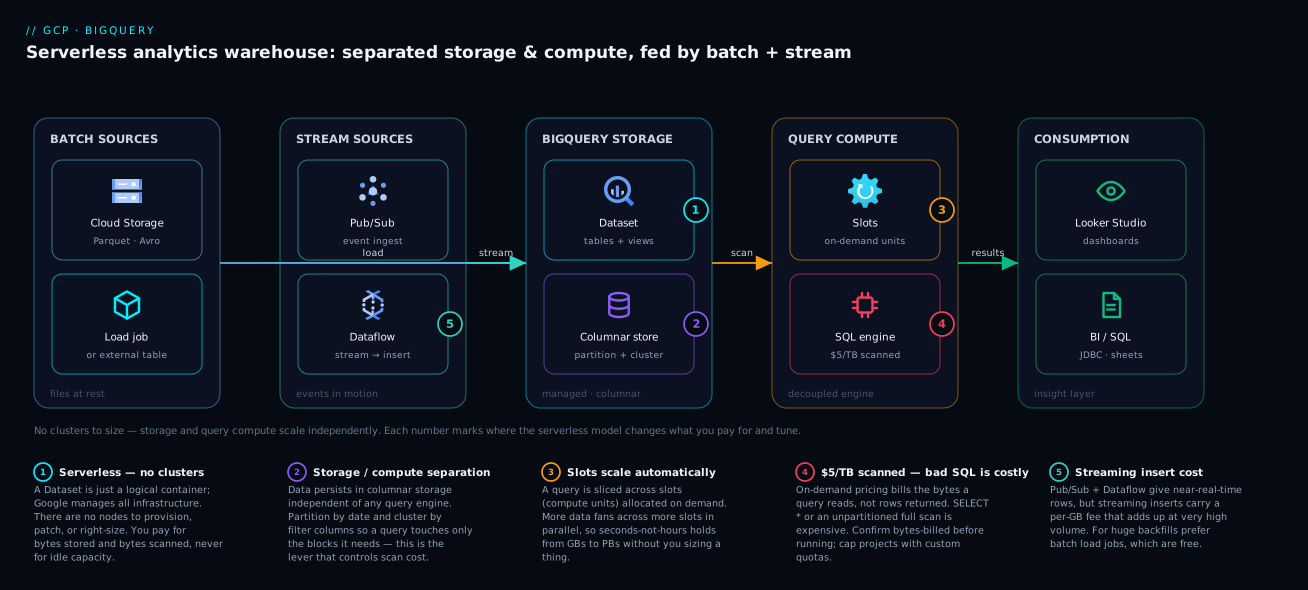
Read the system as two diagrams. The first is the anatomy: data sources on the left (Cloud Storage files, Pub/Sub streams, external sources) flow into BigQuery through the right ingestion path for each — batch load jobs for files (free), the Storage Write API for streams (per-GB), and external/BigLake tables that leave data in GCS and query it in place. Inside BigQuery, the diagram splits the platform into its two independent halves: the storage layer (Capacitor columnar format on Colossus, with your tables partitioned by date and clustered by high-cardinality columns) and the compute layer (the Dremel engine drawing slots from either an elastic on-demand pool or a bought reservation). On the right, results fan out to consumers — Looker Studio and BI tools (accelerated by BI Engine), the Storage Read API for data apps, and materialized views that precompute hot aggregations. The whole picture is the storage/compute separation made visual: the two boxes never touch the same bill.
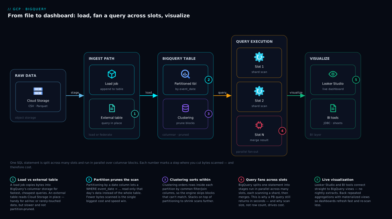
The second diagram is the query data-flow: it traces a single query left-to-right through its lifecycle — submitted SQL is parsed and planned (the optimizer estimating bytes and pruning partitions/columns), slots are scheduled, stages execute in parallel across slots reading only the needed columns and partitions from Capacitor, a shuffle exchanges intermediate data, the final stage aggregates, and the result returns (cached free for 24 hours if eligible). The numbered hops map to where cost is decided: column selection and partition/clustering pruning cut the bytes scanned at the read stage, and the dry-run estimate happens at the plan stage before any byte is billed.
Real-world scenario
Northwind Retail (a fictional but representative mid-size e-commerce company) runs a clickstream and orders warehouse in BigQuery: an events table at roughly 4 TB / 1.2 billion rows per year, plus orders, customers, and inventory. Their analytics started cheap and then the monthly BigQuery bill jumped from about ₹35,000 to ₹2.1 lakh in one billing cycle with no new data volume. The CFO asked the obvious question: what changed?
Nothing in the data — everything in the queries. Three things had quietly gone wrong. First, the events table was unpartitioned: every analyst query that filtered “last 7 days” still scanned the full 4 TB because BigQuery had no partition to prune. Second, a new Looker Studio executive dashboard ran an hourly SELECT *-style aggregate over events — 4 TB × 24 hours/day × 30 days, an enormous scan multiplied by frequency. Third, a junior analyst’s saved query did SELECT * to “explore,” reading all 200 columns when it needed three. None of these were bugs in the SQL — they all returned correct answers. They were design mistakes, each one billed at $5/TB.
The fix took an afternoon and three changes. One — partition and cluster the fact table. They recreated events as PARTITION BY DATE(event_time) CLUSTER BY country, event_type with require_partition_filter = TRUE. Overnight, every “last 7 days” query dropped from scanning 4 TB to about 12 GB — the partition filter that was now mandatory pruned 363 of 365 days. Two — a materialized view for the dashboard. They created daily_revenue as an MV refreshing every 30 minutes; the hourly dashboard now read a few thousand pre-aggregated rows instead of re-scanning 4 TB, and BI Engine made it sub-second. Three — guardrails. They set a project default maximum_bytes_billed of 100 GB and a per-user daily quota of 2 TB, and added a Cloud Billing budget alert at ₹50,000. The junior analyst’s SELECT * now failed with a clear bytes-limit error, teaching the lesson cheaply.
The next month’s bill came in at ₹41,000 — back to baseline plus a little for the MV refresh and BI Engine memory. Same data, same questions, same dashboards: a 5× reduction from partitioning, clustering, one materialized view, and three guardrails. The lasting lesson the team wrote into their onboarding doc: in BigQuery, the query is free to write and the scan is what costs — so the cheapest optimization is almost always a partition filter you forgot, not a bigger reservation.
Advantages and disadvantages
| Advantages | Disadvantages |
|---|---|
| Serverless — no cluster to size, tune, patch, or scale | Per-query cost grows with bytes scanned; a bad query is expensive |
| Storage/compute separation — pay only for what you store + query | Not transactional — no fast point lookups or high-frequency row updates |
| Massive parallelism — TB–PB queries in seconds | On-demand cost is unpredictable without guardrails |
| Columnar + partitioning + clustering → cheap if designed well | Streaming (Storage Write API) costs per-GB, unlike free batch loads |
| Standard SQL, plus BigQuery ML, geospatial, search | Cold/rarely-queried data still incurs storage (cheaper, not free) |
| 24h free result cache; long-term storage auto-discount | Optimization knowledge required — careless SQL bills directly |
| Rich ecosystem (GCS, Pub/Sub, Dataflow, Looker, BI Engine) | Cross-region queries restricted; datasets are location-pinned |
When the advantages dominate: analytical workloads — reporting, dashboards, ad-hoc SQL, ML — over large datasets where elasticity and zero infra management are worth more than micro-optimizing per-query cost (which partitioning handles anyway). When the disadvantages bite: if you need OLTP (use Cloud SQL/Spanner), if your team has no cost discipline and you skip guardrails (the on-demand bill will surprise you), or if everything must be fresh-to-the-second at huge volume (streaming costs add up — batch what you can). The disadvantages are almost all manageable: partitioning kills the scan-cost problem, guardrails kill the unpredictability, and “not transactional” is a feature, not a bug, for an analytics warehouse.
Hands-on lab
Build a partitioned, clustered table, load data, prove pruning with a dry run, set a cost cap, create a materialized view, and tear it all down. Free-tier-friendly: loads are free, and every scan here is well under the 1 TB/month free tier — total cost effectively ₹0. Run in Cloud Shell (which has bq and gcloud preinstalled).
Step 1 — Set your project and create a dataset.
gcloud config set project YOUR_PROJECT_ID
bq --location=US mk --dataset --description "BigQuery lab" lab
# Expected: "Dataset 'YOUR_PROJECT_ID:lab' successfully created."
Step 2 — Create a partitioned + clustered table with the guardrail.
bq query --use_legacy_sql=false '
CREATE TABLE lab.events (
  event_id   STRING,
  user_id    STRING,
  event_type STRING,
  country    STRING,
  amount     NUMERIC,
  event_time TIMESTAMP
)
PARTITION BY DATE(event_time)
CLUSTER BY country, event_type
OPTIONS (require_partition_filter = TRUE);'
# Expected: a success message; the table now exists, empty.
Step 3 — Insert sample rows across several days.
bq query --use_legacy_sql=false '
INSERT INTO lab.events (event_id, user_id, event_type, country, amount, event_time)
SELECT
  GENERATE_UUID(),
  CONCAT("u", CAST(MOD(n, 500) AS STRING)),
  IF(MOD(n,3)=0, "purchase", "view"),
  ["IN","US","UK","SG"][OFFSET(MOD(n,4))],
  ROUND(RAND()*100, 2),
  TIMESTAMP_SUB(CURRENT_TIMESTAMP(), INTERVAL MOD(n, 10) DAY)
FROM UNNEST(GENERATE_ARRAY(1, 5000)) AS n;'
# Expected: "Number of affected rows: 5000."
Step 4 — Prove require_partition_filter works (this query should FAIL).
bq query --use_legacy_sql=false 'SELECT COUNT(*) FROM lab.events;'
# Expected ERROR: "Cannot query over table 'lab.events' without a filter
# over column(s) 'event_time' that can be used for partition elimination."
That error is the guardrail doing its job — it just prevented a full-table scan.
Step 5 — Run a pruning query, and dry-run it first to see the bytes.
# Dry run: see bytes WITHOUT executing
bq query --use_legacy_sql=false --dry_run '
SELECT country, COUNT(*) AS purchases, SUM(amount) AS revenue
FROM lab.events
WHERE DATE(event_time) >= DATE_SUB(CURRENT_DATE(), INTERVAL 3 DAY)
  AND event_type = "purchase"
GROUP BY country;'
# Expected: "... will process N bytes" (tiny — only the last-3-days partitions)

# Now run it for real
bq query --use_legacy_sql=false '
SELECT country, COUNT(*) AS purchases, SUM(amount) AS revenue
FROM lab.events
WHERE DATE(event_time) >= DATE_SUB(CURRENT_DATE(), INTERVAL 3 DAY)
  AND event_type = "purchase"
GROUP BY country;'
# Expected: a small result grouped by country.
Step 6 — Set a bytes cap and watch it block an over-budget query.
bq query --use_legacy_sql=false --maximum_bytes_billed=1000 '
SELECT country, COUNT(*) FROM lab.events
WHERE DATE(event_time) >= DATE_SUB(CURRENT_DATE(), INTERVAL 3 DAY)
GROUP BY country;'
# Expected ERROR: "Query exceeded limit for bytes billed: 1000." — the cap held.
Step 7 — Create a materialized view and query it.
bq query --use_legacy_sql=false '
CREATE MATERIALIZED VIEW lab.daily_revenue AS
SELECT DATE(event_time) AS day, country, SUM(amount) AS revenue
FROM lab.events
WHERE event_type = "purchase"
GROUP BY day, country;'

bq query --use_legacy_sql=false '
SELECT * FROM lab.daily_revenue
WHERE day >= DATE_SUB(CURRENT_DATE(), INTERVAL 3 DAY)
ORDER BY day DESC;'
# Expected: precomputed daily revenue per country.
Step 8 — Inspect what your queries actually billed.
bq query --use_legacy_sql=false '
SELECT job_id, total_bytes_billed, total_slot_ms, cache_hit
FROM `region-us`.INFORMATION_SCHEMA.JOBS_BY_PROJECT
WHERE creation_time > TIMESTAMP_SUB(CURRENT_TIMESTAMP(), INTERVAL 1 HOUR)
  AND statement_type = "SELECT"
ORDER BY creation_time DESC LIMIT 10;'
# Expected: your recent queries with bytes billed (small) and slot-ms.
Validation checklist. You created a partitioned + clustered table, watched require_partition_filter reject a full scan, used a dry run to see bytes before running, watched maximum_bytes_billed block an over-budget query, built a materialized view, and read real billed bytes from INFORMATION_SCHEMA. Every cost lever in the article, exercised end to end. What each step proved:
| Step | What you did | What it proves |
|---|---|---|
| 2 | Partition + cluster + require_partition_filter |
The production fact-table recipe |
| 4 | Un-filtered query rejected | The guardrail prevents full scans |
| 5 | Dry-run then real run | See cost before paying it |
| 6 | maximum_bytes_billed blocks a query |
The per-query seatbelt works |
| 7 | Materialized view | Repeated aggregations get cheap |
| 8 | INFORMATION_SCHEMA.JOBS |
You can audit real bytes billed |
Teardown.
bq rm -r -f --dataset lab
# Removes the dataset and everything in it. Storage charges stop immediately.
Common mistakes & troubleshooting
The failure modes that actually cost teams money and time, as a scannable table, then the worst offenders expanded.
| # | Symptom | Root cause | Confirm (exact cmd / path) | Fix |
|---|---|---|---|---|
| 1 | Query bill far higher than expected | SELECT * reads all columns |
Dry-run: bq query --dry_run ... shows huge bytes; check query in INFORMATION_SCHEMA.JOBS |
Select only needed columns |
| 2 | “Last 7 days” query still scans the whole table | Table not partitioned, or filter doesn’t prune | Dry-run shows full-table bytes; check table DDL for PARTITION BY |
Partition by date; filter the partition column directly |
| 3 | Dashboard quietly bills thousands/month | Frequent query × large scan (hourly SELECT *) |
INFORMATION_SCHEMA.JOBS top total_bytes_billed by query |
Materialized view + BI Engine; reduce frequency |
| 4 | Query rejected: “without a filter over column(s)…” | require_partition_filter=TRUE + no partition filter |
The error names the partition column | Add WHERE <partition_col> … (working as intended) |
| 5 | Query fails: “exceeded limit for bytes billed” | maximum_bytes_billed cap tripped |
Error states the limit | Reduce scan (partition/columns) or raise cap deliberately |
| 6 | Partition filter present but no pruning | Filter wraps the column in a function that hides it | Dry-run bytes ≈ full table despite a WHERE |
Filter the raw column; avoid opaque expressions on it |
| 7 | Streaming costs surprisingly high | Streaming data that didn’t need to be fresh | Billing: streaming/Storage Write API GB | Batch-load what isn’t truly real-time |
| 8 | resourcesExhausted on a big query |
Huge sort/aggregate/ORDER BY over too much data |
Job error; query plan shows a massive final stage | Filter more; avoid global ORDER BY on huge sets; add LIMIT/partition |
| 9 | Slow query on a reservation, low CPU | Queued waiting for slots (reservation too small) | total_slot_ms high vs wall time; slots maxed |
Add slots / autoscale; isolate workloads |
| 10 | Cross-region query error | Dataset and destination in different locations | Error: “Cannot read in location X…” | Co-locate datasets; copy/transfer across regions |
| 11 | Costs creep with no obvious cause | No project default cap, no quotas | No maximum_bytes_billed default; no custom quota |
Set project default cap + per-user daily quota + budget alert |
| 12 | Repeated identical query still bills | Cache busted by CURRENT_TIMESTAMP()/changing table |
cache_hit=false in INFORMATION_SCHEMA.JOBS |
Remove non-deterministic fns; stabilize inputs |
The three that bite hardest, expanded:
1. SELECT * is a financial event. Because storage is columnar and billing is per-byte-scanned, SELECT * reads every column — often 50× more bytes than the three columns you actually use. Confirm: a dry run shows the bytes; INFORMATION_SCHEMA.JOBS reveals the offending query text. Fix: select only the columns you need, every time. In a dashboard or pipeline, never SELECT *. (SELECT * EXCEPT(big_col) still reads everything except the named columns — it’s a partial fix; explicit column lists are the real one.)
2. The unpartitioned fact table. A large table without PARTITION BY cannot prune by date — every “recent data” query scans all history. Confirm: dry-run a “last 7 days” query; if it reports near the full table size, there’s no pruning. Check the DDL (bq show --schema / the table details) for a partitioning spec. Fix: recreate the table PARTITION BY DATE(...), add CLUSTER BY the next-most-filtered columns, set require_partition_filter = TRUE, and migrate the data with a single CREATE TABLE ... AS SELECT.
3. The hourly dashboard scanning terabytes. Cost = bytes × frequency. A correct query over a 4 TB table, run hourly, is 96 TB/day. Confirm: INFORMATION_SCHEMA.JOBS grouped by query shows the same query repeating with a huge total_bytes_billed. Fix: back the dashboard with a materialized view (precomputed, incrementally refreshed) and accelerate with BI Engine so it serves from memory; reduce refresh frequency to what the business actually needs.
Best practices
- Never
SELECT *in production. Name the columns. It’s the single biggest scan-cost reducer and it makes queries cacheable and readable. - Partition every large time-series table by its event/ingestion date, and set
require_partition_filter = TRUEso an un-pruned scan is rejected, not billed. - Cluster on the two-to-four columns you filter and join on most, in priority order, on top of partitioning. It’s free to maintain and skips blocks.
- Always filter the partition column directly —
WHERE event_time >= ...— and avoid wrapping it in functions that defeat pruning. - Dry-run new and large queries, and gate pipeline queries on a dry-run bytes check in CI.
- Set
maximum_bytes_billedas a project default and let power users raise it deliberately; add per-user and per-project daily quotas. - Batch-load what isn’t truly real-time (loads are free) and reserve the per-GB Storage Write API for data that genuinely needs seconds-fresh latency.
- Back repeated aggregations with materialized views, and accelerate fixed dashboards with BI Engine — don’t re-scan the base table on every refresh.
- Prefer Parquet/Avro for loads (columnar, schema-carrying, fast) over CSV.
- Co-locate datasets in one region to avoid cross-region query restrictions and egress; pick the region close to your users/sources.
- Audit weekly with the “top queries by
total_bytes_billed” query againstINFORMATION_SCHEMA.JOBS— it finds the runaway dashboard before the invoice does. - Decide on-demand vs reservation by measured monthly scan, not by guess: stay on-demand until steady volume justifies a small committed reservation, then re-measure.
Security notes
- Least-privilege IAM on datasets. Grant roles at the dataset (or table/column) level, not blanket
bigquery.adminon the project. Useroles/bigquery.dataViewerfor read,roles/bigquery.dataEditorfor write, androles/bigquery.jobUserto run queries (running a query is a separate permission from reading data). Build on Google Cloud IAM Explained Simply. - Column-level and row-level security (Enterprise edition): tag sensitive columns with policy tags (via Data Catalog) so only authorized principals can read PII columns, and apply row-level access policies so each team sees only its rows — without separate tables.
- Authorized views and BigLake let consumers query results without direct access to underlying tables/files — share an aggregate without exposing raw PII.
- CMEK (customer-managed encryption keys via Cloud KMS) for datasets when compliance requires you to hold the key; BigQuery encrypts at rest by default regardless.
- VPC Service Controls wrap BigQuery in a perimeter so data can’t be exfiltrated to projects outside the boundary — essential for regulated data; see GCP VPC Service Controls.
- Audit with Cloud Audit Logs (Data Access logs) to see exactly who queried what, and pipe them to a monitored sink.
The access-control surface, who each piece protects, and the role/mechanism:
| Control | Protects | Role / mechanism | Edition |
|---|---|---|---|
| Dataset IAM | Who reads/writes a dataset | dataViewer / dataEditor |
All |
| Job/query permission | Who can run queries | roles/bigquery.jobUser |
All |
| Column-level security | Sensitive columns (PII) | Policy tags (Data Catalog) | Enterprise |
| Row-level security | Per-row visibility | Row access policies | Enterprise |
| Authorized views / BigLake | Sharing results w/o raw access | View/BigLake delegation | All / BigLake |
| CMEK | Encryption key custody | Cloud KMS key on dataset | All |
| VPC Service Controls | Exfiltration to outside projects | Service perimeter | All |
Cost & sizing
What drives the BigQuery bill, in order of how often it surprises people:
- Query compute is the variable that bites. On-demand is $5/TB scanned, with the first 1 TB/month free. The bill is bytes × frequency — so a partition-pruned query is cheap even run often, and an unpartitioned one is expensive even run rarely. Everything in the partitioning section exists to shrink this number.
- Storage is the quiet, predictable line: ~$0.02/GB/month active, ~$0.01/GB/month long-term (auto-applied after 90 days untouched, per partition). 10 TB stored ≈ $200/month active, dropping toward $100 as partitions age out. Cheap relative to compute for most teams.
- Streaming ingestion (Storage Write API) is per-GB ingested — real but usually small unless you stream everything. Batch loads are free.
- BI Engine is reserved memory/hour; reservations are slot-hours. Both are flat, predictable spend you opt into for performance/predictability.
Sizing guidance: start on-demand (zero idle cost), make partitioning and maximum_bytes_billed your cost control, and only price a reservation once steady monthly scan is high enough that slot-time beats per-byte (typically tens-to-hundreds of TB/month). Use long-term storage automatically (do nothing — it just happens) and partition expiration to drop ancient data. The cost drivers and the lever for each:
| Cost driver | What you pay | Rough figure | Lever to reduce it |
|---|---|---|---|
| On-demand query | $5 / TB scanned (1 TB/mo free) | ₹420 per TB | Partition, cluster, select fewer columns |
| Active storage | ~$0.02/GB/month | ₹1.7/GB/mo | Partition expiration; physical billing if very compressible |
| Long-term storage | ~$0.01/GB/month (auto) | ₹0.85/GB/mo | Automatic after 90 days untouched |
| Streaming (Write API) | Per-GB ingested | small | Batch what isn’t truly real-time |
| BI Engine | Reserved memory / hour | flat | Size to the hot working set only |
| Reservation (Editions) | Slot-hours (commit/autoscale) | flat | Right-size slots; workload isolation |
| Free tier | 1 TB scan + 10 GB storage / month | ₹0 | Keep dev/exploration under it |
A rough monthly picture for Northwind-scale (10 TB stored, modest well-partitioned querying): storage ~₹17,000 (dropping as partitions age) + query ~₹15,000–40,000 depending on discipline — and the entire swing in that query number is whether the team partitions and guards or runs SELECT * hourly. The cheapest optimization in BigQuery is almost always free: a partition filter and an explicit column list.
Interview & exam questions
1. Why does SELECT * cost more than selecting three columns in BigQuery? Storage is columnar (Capacitor), so a query reads only the columns it references; SELECT * reads every column’s bytes. On-demand billing is $5 per TB of bytes scanned, so reading 200 columns instead of 3 can cost ~50× more for the same rows. The result size is irrelevant — bytes processed is what bills.
2. Explain BigQuery’s storage/compute separation and why it matters for cost. Data lives in Colossus (columnar Capacitor format) and compute runs on the separate Dremel engine using slots. They scale and bill independently, so a large table costs almost nothing between queries (storage only) and a query summons elastic compute just for its duration. It means idle cost is near zero and query cost is purely a function of bytes scanned.
3. Partitioning vs clustering — what does each do? Partitioning splits a table into segments by a date/timestamp or integer column; a filter on that column prunes whole partitions (exact, hard pruning). Clustering sorts data within partitions by up to four columns; a filter on a clustered column skips blocks that can’t match (approximate block pruning). Production pattern: partition by date, cluster by the next-most-filtered columns.
4. On-demand vs Editions reservations — when do you choose each? On-demand ($5/TB scanned, zero idle cost) suits spiky, ad-hoc, lower-volume workloads. Reservations (bought slot-time) suit steady, high-volume workloads needing predictable cost and guaranteed/bounded capacity. The break-even is when steady monthly scan is high enough (tens–hundreds of TB) that slot-time beats per-byte. On-demand risks a runaway-query bill; reservations risk a runaway-query slowdown.
5. What is a slot? A slot is BigQuery’s unit of compute — a worker share executing one unit of a query’s parallel plan. On-demand grants an elastic slot pool transparently and bills only bytes; with reservations you buy a fixed number of slots and queries share (and may queue against) them. Concurrency on a reservation is bounded by slots owned.
6. How do you prevent a single query from scanning terabytes by accident? Layer guardrails: require_partition_filter = TRUE on the table rejects un-pruned scans; a dry run shows bytes before running; maximum_bytes_billed fails a query that would exceed a byte ceiling; per-user/project daily quotas cap aggregate scan; and a Cloud Billing budget alert notifies on threshold. Together they make a shocking invoice impossible.
7. What does a dry run tell you and how is it billed? A dry run plans the query and reports the bytes it would scan without executing it or billing anything. It’s the design-time check to catch an expensive scan before paying for it — and the basis for a CI cost gate on pipeline queries.
8. When would you use an external table instead of loading data? When you want to query data in place in Cloud Storage without copying it into BigQuery — occasional queries, a staging view before a real load, or to avoid a second storage copy. You still pay $5/TB to scan, lose native Capacitor speed, and get limited pruning. For governed in-place data with row/column security, use BigLake.
9. What’s the difference between a materialized view and BI Engine? A materialized view precomputes and stores a specific aggregation, refreshing incrementally as the base table changes; querying it (or the base table, via transparent rewrite) reads the small precomputed result. BI Engine is an in-memory cache that accelerates whatever a dashboard touches to sub-second. They compose: dashboards on MVs, accelerated by BI Engine.
10. Why is BigQuery a poor choice for an application’s point lookups? It’s analytical, not transactional — built to scan and aggregate huge datasets, with no indexes for fast single-row reads and comparatively expensive per-row DML. A WHERE id = 42 for an app belongs in Cloud SQL/Spanner/Bigtable, which serve millisecond point reads and high-frequency writes.
11. How does the query result cache save money, and what defeats it? An identical query (same text) over unchanged data returns from a 24-hour result cache for free and instantly. It’s defeated by any change to a referenced table, by non-deterministic functions (CURRENT_TIMESTAMP(), RAND()), and (effectively) by SELECT * on a frequently-changing table. Keep cacheable queries deterministic.
12. Why do batch loads cost nothing while streaming costs per-GB? Load jobs run on shared infrastructure and BigQuery doesn’t charge query/compute for them — you pay only for the resulting storage. Streaming (Storage Write API) provides near-real-time, exactly-once ingestion at a per-GB charge for that capability. So batch what can tolerate minutes of latency; stream only what truly needs seconds.
These map to the Google Cloud Professional Data Engineer certification (BigQuery design, partitioning/clustering, cost optimization, loading, security) and touch the Associate Cloud Engineer (basic BigQuery operation, IAM). A compact cert mapping:
| Question theme | Primary cert | Objective area |
|---|---|---|
| Architecture, slots, storage/compute | PDE | Designing data processing systems |
| Partitioning, clustering, cost control | PDE | Operationalizing & optimizing |
| Loading, streaming, external/BigLake | PDE | Ingesting & processing data |
| IAM, column/row security, VPC-SC | PDE / PCA | Security & compliance |
| Basic dataset/table ops, querying | ACE | Deploying & monitoring resources |
Quick check
- You run
SELECT user_id, amount FROM events WHERE DATE(event_time) = "2026-06-23"on a daily-partitioned table that holds 365 days of data. Roughly what fraction of the table do you scan, and why? - True or false: scanning 4 TB but returning only 10 rows costs the same as scanning 4 TB and returning a million rows.
- Name the two table-design features that reduce bytes scanned, and the difference between them.
- Which one setting on a table will reject a query that doesn’t filter the partition column, and why would you want that?
- Your dashboard re-runs the same expensive aggregation every 30 minutes. Name two features that make it cheap, and what each does.
Answers
- About 1/365 of the table — the partition filter on
event_timeprunes to a single day’s partition, and you read only two columns of it. Partition pruning plus column pruning is why it’s cheap. - True. On-demand billing is by bytes scanned (processed), not by rows returned. Both queries scan 4 TB, so both cost the same (~₹1,700); the result size is irrelevant to the bill.
- Partitioning (splits the table into segments by a date/int column; a filter prunes whole partitions — exact) and clustering (sorts data within partitions by ≤4 columns; a filter skips blocks that can’t match — approximate). Partition first, then cluster on the next-most-filtered columns.
require_partition_filter = TRUE. It rejects any query lacking a filter on the partition column, preventing accidental full-table scans before they bill — the cheapest guard against the “last 7 days” query that secretly scans everything.- A materialized view (precomputes and incrementally refreshes the aggregation, so reads hit a small stored result instead of the base table) and BI Engine (holds hot data in memory so the dashboard serves sub-second, with cache-served bytes effectively free). Together: dashboard on the MV, accelerated by BI Engine.
Glossary
- Project — the billing and IAM boundary; datasets live inside it and queries are billed to it.
- Dataset — a region-pinned container for tables and views; the unit of access control and location.
- Table — a columnar collection of rows; the object you scan, optionally partitioned and clustered.
- Capacitor — BigQuery’s compressed columnar storage format; the reason only referenced columns are read.
- Colossus — Google’s distributed file system where table bytes physically live, replicated across zones.
- Dremel — the multi-tenant query execution engine that runs your SQL in parallel across slots.
- Slot — the unit of compute (a worker/CPU-RAM share); elastic on-demand, or bought via reservations.
- Partition — a table segment defined by a date/timestamp or integer column; filters prune partitions to cut scan.
- Clustering — the sort order of data within partitions by up to four columns; filters skip non-matching blocks.
- Bytes processed / billed — the uncompressed bytes a query reads; what on-demand pricing charges ($5/TB).
- On-demand pricing — pay $5 per TB scanned (first 1 TB/month free), no slot management, zero idle cost.
- Editions / reservation — pay for bought slot-time (Standard/Enterprise/Enterprise Plus) for predictable cost and bounded concurrency.
maximum_bytes_billed— a per-query hard cap; a query that would exceed it fails before running.require_partition_filter— a table option that rejects any query without a partition-column filter.- Dry run — a plan-only execution that reports bytes-to-be-scanned without running or billing.
- Materialized view — a precomputed, incrementally auto-refreshed aggregation stored for cheap repeated reads.
- BI Engine — an in-memory acceleration layer that serves hot dashboard data sub-second.
- External table — a table over files left in Cloud Storage (etc.), queried in place; scan-priced, no copy.
- BigLake — governed external tables adding row/column security and access delegation (lakehouse pattern).
- Storage Write API — the modern per-GB streaming ingestion API for near-real-time, exactly-once writes.
- Result cache — a free 24-hour cache returning identical queries over unchanged data instantly.
- Long-term storage — the automatic ~50% storage discount on any table/partition untouched for 90 days.
Next steps
You can now design a BigQuery warehouse that’s fast and cheap by construction, load it four ways, and guard it against runaway cost. Build outward:
- Next: BigQuery for Beginners: How Serverless Analytics Works and the $5/TB Cost Model — reinforce the cost mental model from first principles.
- Related: GCP Pub/Sub and Event-Driven Architecture — the streaming source that feeds the Storage Write API for real-time ingestion.
- Related: Cloud Storage Classes Decoded: Standard, Nearline, Coldline, Archive — the staging layer for almost every batch load.
- Related: GCP Cloud Monitoring and Operations — watch slot utilization, bytes billed, and set alerts on cost signals.
- Related: Google Cloud IAM Explained Simply — lock datasets down with least-privilege roles and column/row security.
- Related: GCP VPC Service Controls: Build Data Exfiltration Perimeters — wrap BigQuery in a perimeter for regulated data.