You loaded a year of web-traffic logs into BigQuery, ran SELECT * FROM events WHERE event_date = '2026-06-01' to peek at one day, and the answer came back in four seconds across two billion rows. It felt like magic — no cluster to spin up, no “warming up”, no nodes to size. Then, at the end of the month, the bill had a line you didn’t expect: that one casual query, and a few hundred like it, had quietly cost you more than the rest of your Google Cloud account combined. Nobody warned you, because BigQuery doesn’t make you provision anything — so there’s no slider that says “this is how much you’re about to spend.”
This article is the mental model that prevents that surprise. BigQuery is Google’s serverless data warehouse — a place to store enormous tables (think billions or trillions of rows) and ask them questions in plain SQL, where Google runs the machines for you and hands you back answers in seconds. “Serverless” is the part everyone loves and the part that bites: because you never see a server, you also never see the meter. The price isn’t “per VM per hour” like most cloud things — in the default on-demand mode it’s $5 per terabyte of data your query reads, and the trap is that a tiny-looking query can read a giant amount of data without telling you first. The whole game is learning to see, before you press run, how much data a query will touch.
By the end you will hold two things firmly: (1) a clear picture of how a serverless query runs — what happens in those four seconds, where your data physically lives, why it scales without you lifting a finger — and (2) a working model of how the bill is computed, down to the column, so you can look at any query and say “two cents” or “stop, that’s a thirty-dollar SELECT *.” Concrete analogies, real bq and gcloud commands, a Terraform snippet, and worked dollar math — no hand-waving, no jargon dumps, just the model made obvious.
What problem this solves
Before BigQuery, “analytics at scale” meant running a data warehouse cluster — a fixed set of beefy machines you bought (or rented by the hour) and kept running so they’d be ready when someone asked a question. That model has three chronic pains: you size for the peak and pay for the trough (the cluster is sized for month-end, then sits mostly idle 24×7 — like renting a 40-seat bus for the one trip a month the whole team travels); someone has to run it (patching, scaling, backups, upgrades — a person’s job); and big questions choke, because only the nodes you provisioned can help, so speed is rigidly coupled to a number you set in advance.
BigQuery dissolves all three by separating storage from compute and making both elastic. Your data sits in cheap, durable storage that’s always there. When you run a query, Google temporarily borrows however many machines that query needs from a giant shared pool — a dozen or thousands — runs it, and hands them back the instant it’s done. You pay for the work the query did, measured as bytes read, not for idle machines. Nothing to size, run, or patch.
Here’s the catch this article exists to handle: removing the cluster also removed the visible cost ceiling. With a fixed cluster, your bill was capped — you couldn’t spend more than your nodes cost, no matter how careless the SQL. With BigQuery on-demand, every query spends money in proportion to the data it reads, and a careless query can read a lot. You’re trading cluster-management skill for cost-awareness per query — a much easier skill, but only if someone teaches it to you, which almost nobody does until the bill arrives.
| Old world (cluster warehouse) | BigQuery world (serverless) | What changed for you |
|---|---|---|
| Buy/rent fixed nodes, run 24×7 | No nodes; Google runs a shared fleet | Stop paying for idle hardware |
| Size for peak, waste the trough | Compute borrowed per-query, returned after | Pay for work done, not capacity owned |
| You patch/scale/upgrade the cluster | Google operates everything | No ops team needed |
| Speed tied to node count you set | A big query pulls in thousands of workers | Big questions finish in seconds |
| Bill is capped by node cost | Bill scales with bytes each query reads | New skill: see cost before you run |
| Storage and compute on same boxes | Storage and compute fully separate | Store cheaply forever; pay compute only when querying |
Learning objectives
By the end of this article you can:
- Explain in one sentence what “serverless” means for BigQuery and why it changes how you pay, not just how you operate.
- Walk through what physically happens in the seconds between pressing Run and getting an answer — storage, the worker fleet, the shuffle, and the result.
- Describe BigQuery’s columnar storage and explain why reading 2 of 50 columns costs roughly 1/25th as much as reading all of them.
- Calculate the cost of any on-demand query yourself: bytes scanned ÷ 1 TB × $5, and read the dry-run estimate before you spend a cent.
- Recognise the four habits that cause surprise bills —
SELECT *, no partition filter, re-running the same scan, andLIMITnot saving you — and the fix for each. - Choose correctly between on-demand pricing and capacity (slots) pricing using a simple break-even rule.
- Cut a query’s cost by 10–100× using partitioning and clustering, and know which one does what.
- Set hard guardrails — per-query and per-day billing caps, plus dataset structure — so a careless query can’t run up a four-figure bill.
Prerequisites & where this fits
You need almost nothing to start. A Google Cloud project with billing enabled, the ability to open the Cloud Console or run gcloud / bq in Cloud Shell (a free browser terminal Google gives you), and comfort reading basic SQL — SELECT, FROM, WHERE, GROUP BY. That’s it. You do not need to understand servers, clusters, Hadoop, Spark, or distributed systems; the entire point of BigQuery is that you don’t.
Where this sits in the bigger picture: BigQuery is the analytics / warehouse layer of Google Cloud — the place where data lands after it’s been collected, to be queried and reported on. It is not a transactional database (you don’t run a checkout cart on it); for that you’d reach for Cloud SQL or Firestore. It’s where you ask “how did sales trend across all regions last quarter?” not “charge this one customer $9.99 right now.” If you’ve read the broader GCP picture in GCP Compute: Compute Engine, Cloud Run, GKE and Cloud Functions or The GCP Resource Hierarchy Explained: Organization, Folders, Projects, and Why It Runs Everything, this is the data corner of that map. Coming from another cloud, BigQuery is the rough equivalent of Amazon Redshift / Athena or Azure Synapse — the translation maps in GCP for AWS Engineers: The Complete Service-by-Service Translation Map and GCP for Azure Engineers: How Every Azure Service Maps to Google Cloud place it precisely.
This article is the on-ramp. Once the mental model and cost model click, the natural next stop is the deep mechanics — Google BigQuery, In Depth: Datasets, Tables, Partitioning, Slots & Pricing — and the optimisation craft in Taming BigQuery Cost and Performance: Partitioning, Clustering, and Reservations.
Here’s the one-glance placement of BigQuery against its neighbours, so you never reach for the wrong tool:
| You want to… | Use | Not BigQuery because… |
|---|---|---|
| Analyse billions of rows with SQL | BigQuery | — this is exactly it |
| Power a web app’s logins/orders | Cloud SQL / Firestore | BigQuery isn’t built for tiny fast row writes |
| Cache or sub-millisecond lookups | Memorystore | BigQuery answers in seconds, not microseconds |
| Store raw files (CSV, images, backups) | Cloud Storage | BigQuery stores tables, not arbitrary files |
| Stream events into a pipeline | Pub/Sub → BigQuery | Pub/Sub moves events; BigQuery is the destination |
| Train/serve ML models | Vertex AI (or BigQuery ML for in-SQL models) | Heavy model serving lives elsewhere |
Core concepts
Five ideas unlock everything else. Read these once and the rest of the article is just detail hanging off them.
1. Serverless means the unit you rent is “a query,” not “a machine.” With a normal cloud service you rent a server (or container, or function) and it exists whether or not you use it. With BigQuery you rent the execution of a query — there is no BigQuery server to SSH into, restart, or see in a VM list. Press Run, Google grabs capacity from an enormous shared fleet, runs your SQL, and releases it. The mental shift: stop asking “how big is my machine?” and start asking “how much data will this question read?”
2. Storage and compute are two separate things you pay for separately. This is the single most important structural fact. Your tables live in storage — cheap, durable, billed per gigabyte-month whether or not anyone queries them. Running a query uses compute — billed separately, by work done. They scale independently: store a petabyte and pay zero compute until you query it; run a thousand queries today and none tomorrow and your storage bill doesn’t budge. Newcomers conflate the two and get confused by the bill. Keep them in separate mental buckets.
3. Data is stored by column, not by row — which is why the price model works as it does. A traditional database stores a 50-column table row by row (all 50 values of row 1 together, then row 2…). BigQuery stores it column by column. So SELECT user_id, country reads only those two columns’ blocks and physically skips the other 48 — you read ~2/50ths of the data and pay ~2/50ths of the cost. This is columnar storage, the reason SELECT * can cost 25× more than naming two columns on the same table. (The dedicated section below works this out in dollars.)
4. The on-demand price is “$5 per terabyte of data your query reads.” Not rows. Not time. Not result size. Bytes scanned. BigQuery sums the size of the columns (and partitions) it must read and charges $5 per 1 TB (first 1 TB/month free). 200 GB ≈ $0.98; 50 MB ≈ a fraction of a cent. Crucially, a small result does not make a query cheap — SELECT COUNT(*) FROM huge_table returns one number but may scan the whole table. Cost tracks input read, not output produced.
5. You can see the price before you pay it — always. Every query can be run as a dry run: BigQuery reports exactly how many bytes it would scan, without running it or charging you. The Console shows “This query will process X GB when run”; the CLI uses --dry_run. This is your seatbelt — the entire difference between being surprised by the bill and not is whether you glance at that estimate before pressing Run.
The vocabulary, side by side
Before the deep sections, pin down every term. The glossary at the end repeats these for quick lookup; this table is the mental model in one place.
| Term | Plain-English meaning | Why a beginner cares |
|---|---|---|
| Serverless | You rent query execution, not machines | No sizing, no patching, no idle cost |
| Dataset | A folder that holds tables, in one region | The unit of organisation and access control |
| Table | Your data, in rows and columns | The thing you query |
| Columnar storage | Data stored column-by-column | Reading fewer columns = lower cost |
| Bytes scanned | The data a query physically reads | This is what you’re billed on (on-demand) |
| On-demand pricing | $5 per TB scanned, first 1 TB/mo free | The default; pay per query |
| Slot | A unit of compute (a “worker share”) | What you reserve in capacity pricing |
| Capacity pricing | Pay for slots by time, queries “free” | Cheaper at high, steady volume |
| Dry run | A cost estimate without running | Your seatbelt before pressing Run |
| Partition | A table sliced (usually by date) | A WHERE date= filter skips other slices |
| Clustering | Rows sorted by chosen columns | Lets BigQuery skip blocks within a partition |
| Active vs long-term storage | Tables touched <90 days vs ≥90 days | Untouched data auto-halves in storage price |
How a serverless query actually runs (the four seconds explained)
Let’s slow down those four magic seconds. Understanding the machinery makes the cost model obvious and demystifies why it scales without you.
When you press Run on SELECT country, COUNT(*) FROM events WHERE event_date = '2026-06-01' GROUP BY country, here’s the relay race that happens:
Step 1 — The query planner reads the question. A coordinator parses your SQL, looks at the table’s structure, and works out the cheapest way to answer it. Critically, it decides which data it must read: only the country and event_date columns (columnar storage), and — because the table is partitioned by date — only the one day’s partition, not the whole year. This decision is what the dry-run estimate reflects.
Step 2 — Work is split across many workers. The planner chops the job into thousands of small tasks and hands them to workers (the underlying unit is a slot) pulled from Google’s shared fleet — a few for a small job, thousands for a billion-row scan, all in parallel. You didn’t ask for them, size them, or wait for them to boot; they’re already running, shared across all of Google’s customers, and your slice is allocated and released in real time.
Step 3 — Workers read their slice from storage. Each worker reads its chunk of the country column from Colossus, Google’s distributed storage where your table physically lives (on separate machines from the compute). Storage and compute talk over Jupiter, Google’s ultra-fast internal network — which is why “separate storage and compute” doesn’t make things slow.
Step 4 — The shuffle. To compute GROUP BY country, every “India” row must reach the same worker to be counted together (and so on per country). Workers exchange data in a stage called the shuffle — the part that makes distributed SQL hard, done for you invisibly.
Step 5 — Results assemble and return. Each country’s count is finalised, the small result is gathered, and it appears on screen; the workers go back to the fleet. The bytes you were charged for are those read in Step 3 — not the size of the tiny result.
Here’s that pipeline as a reference, with the cost-relevant note on each stage:
| Stage | What happens | Where it runs | Cost impact |
|---|---|---|---|
| Plan | Parse SQL, pick columns & partitions to read | Coordinator | Determines bytes scanned (the bill) |
| Dispatch | Split into tasks, grab slots from the fleet | Shared worker pool | Free in on-demand; this is what slots are |
| Read | Workers read selected columns from storage | Colossus (storage) | Bytes read here = what you pay for |
| Shuffle | Regroup data across workers (e.g. by GROUP BY key) | Jupiter network | No extra charge; happens for free |
| Aggregate | Compute final results | Workers | No extra charge |
| Return | Assemble result, release workers | Coordinator → you | Result size doesn’t affect cost |
Two takeaways that will save you money for the rest of your BigQuery life: the Plan stage is where your bill is decided (it picks how many bytes get read), and the Read stage is the only one you pay for in on-demand mode. Everything you do to make a query cheaper — selecting fewer columns, filtering to fewer partitions — works by shrinking what the Plan stage decides to read.
Columnar storage: why your column choices are your cost dial
This concept deserves its own section because it’s the lever you’ll pull most often. Let’s make it concrete with a worked example.
Imagine a table events with these characteristics:
- 50 columns
- 2 billion rows
- 1 TB total size on disk
- Each column is, on average, 1/50th of the table ≈ 20 GB (real columns vary — a big JSON blob column might be 400 GB while a boolean is tiny — but assume even for the example)
Now compare three queries on this exact table:
| Query | Columns read | Bytes scanned | On-demand cost |
|---|---|---|---|
SELECT * FROM events |
all 50 | ~1 TB | ~$5.00 |
SELECT user_id, country, event_date FROM events |
3 | ~60 GB | ~$0.29 |
SELECT country FROM events |
1 | ~20 GB | ~$0.10 |
Same table. Same two billion rows. The cost ranges from ten cents to five dollars — a 50× swing — decided entirely by which columns you name. This is why the very first rule of BigQuery is never SELECT * on a wide or large table unless you genuinely need every column. SELECT * isn’t just sloppy here; it’s the most expensive thing you can type.
A subtle and important corollary: LIMIT does not reduce cost in on-demand mode. New users assume SELECT * FROM events LIMIT 10 is cheap because it returns 10 rows. It is not — to find any 10 rows it still reads the full columns from storage, so it scans ~1 TB and costs ~$5. LIMIT shrinks the result, not the read. (The one exception is the table Preview tab in the Console, which is free because it reads stored metadata, not the query engine.)
| Common assumption | Reality | Why |
|---|---|---|
“LIMIT 10 makes it cheap” |
No — still scans full columns | LIMIT trims output, not input |
“COUNT(*) is tiny, it’s one number” |
Depends — may scan a column or full table | Cost = input read, not output size |
“WHERE always lowers cost” |
Only if it filters a partition or a clustered column | A WHERE on an unindexed column still reads all of it |
| “Small result = small cost” | No correlation | You pay for bytes read, not bytes returned |
| “Sorting is what’s expensive” | No — reading wide columns is | Compute (sort/shuffle) is free in on-demand |
The mental model to lock in: in on-demand BigQuery, you are billed for what you ask it to read, not for what it gives you back. Your SELECT list and your partition filter are the two dials that control “what it reads.” Everything else is free.
The $5/TB cost model, computed by hand
Now the centrepiece. Let’s make you able to price any on-demand query in your head, then verify with the tools.
The formula
on-demand query cost (USD) = (bytes scanned ÷ 1,099,511,627,776) × $5
That divisor is 1 TB in bytes (BigQuery bills in binary terabytes — TiB — so 1 TB = 1024⁴ bytes, ≈ 1.0995 × 10¹²). The first 1 TB per month is free per billing account. So the practical formula most people use:
cost ≈ (TB scanned − 1 free TB this month) × $5
A few anchor points worth memorising so you have intuition without a calculator:
| Bytes scanned | ≈ TB | On-demand cost | Intuition |
|---|---|---|---|
| 10 MB | 0.00001 | ~$0.00005 | Free-tier noise |
| 1 GB | 0.001 | ~$0.0049 | Half a cent |
| 100 GB | 0.098 | ~$0.49 | About fifty cents |
| 1 TB | 1.0 | ~$5.00 | The headline number |
| 10 TB | 10 | ~$50 | A meaningful query |
| 100 TB | 100 | ~$500 | Someone SELECT *'d the warehouse |
| 1 PB | 1024 | ~$5,000 | Call your manager |
See it before you spend it: the dry run
Never guess — measure. Every query can be priced for free with a dry run. In the CLI:
# Estimate bytes WITHOUT running the query or being charged
bq query --use_legacy_sql=false --dry_run \
  'SELECT user_id, country
   FROM `my-project.analytics.events`
   WHERE event_date = "2026-06-01"'
Expected output (the number is what matters):
Query successfully validated. Assuming the tables are not modified,
running this query will process 58720256 bytes of data.
That’s 56 MB → about a quarter of a cent. Compare with the same query but SELECT *:
bq query --use_legacy_sql=false --dry_run \
  'SELECT * FROM `my-project.analytics.events`
   WHERE event_date = "2026-06-01"'
# -> running this query will process 21474836480 bytes of data.
That’s 20 GB → about ten cents for one day — and on a full-year scan it would be the whole table. The dry run turned an invisible decision into a visible number. Make --dry_run (or glancing at the Console’s “will process X” estimate) a reflex before any query on an unfamiliar or large table.
You can also script the conversion to dollars:
BYTES=$(bq query --use_legacy_sql=false --dry_run --format=json \
  'SELECT user_id, country FROM `my-project.analytics.events`
   WHERE event_date = "2026-06-01"' \
  | python3 -c 'import sys,json; print(json.load(sys.stdin)["statistics"]["totalBytesProcessed"])')
python3 -c "print(f'Scan: {int($BYTES)/2**40:.4f} TB  ~= \${int($BYTES)/2**40*5:.4f}')"
# Scan: 0.0001 TB  ~= $0.0003
A worked monthly example
Let’s price a realistic small analytics workload so the numbers feel real. Suppose your team runs a dashboard that refreshes hourly off a 30-day partitioned events table, plus some ad-hoc analysis.
| Workload item | Scan per run | Runs/month | Monthly TB | On-demand cost |
|---|---|---|---|---|
| Hourly dashboard (reads 1 day’s partition, 4 cols) | 5 GB | 720 | 3.52 TB | ~$17.58 |
| Daily exec report (reads 30-day, 6 cols) | 80 GB | 30 | 2.34 TB | ~$11.72 |
| Ad-hoc analyst queries | ~50 GB avg | 200 | 9.77 TB | ~$48.83 |
| Subtotal | 15.63 TB | ~$78.13 | ||
| Less 1 TB free tier | −1 TB | −$5.00 | ||
| Estimated monthly query cost | ~$73.13 |
Add storage (say 1 TB of data ≈ $20/month active storage, less if some is long-term), and your all-in BigQuery bill is roughly $93/month (~₹7,800). Now look at what one bad habit does to that table: if the analyst queries were SELECT * on a 50-column table instead of 6 columns, the ad-hoc line alone jumps from 9.77 TB to ~81 TB, and the monthly bill rockets past $400. Same insights, 4× the cost, entirely from column hygiene. That is the surprise this article is named after.
On-demand vs capacity (slots): which pricing model to pick
So far everything has been on-demand — the default, pay-$5-per-TB-scanned model. There’s a second model, capacity (a.k.a. slot reservations / BigQuery Editions), and choosing right can halve your bill. Here’s the plain version.
On-demand = “pay per query, by bytes scanned.” No commitment, perfect for getting started, spiky usage, and small teams. Its risk is unpredictability — a busy month or a careless SELECT * spree shows up directly on the bill.
Capacity = “rent a fixed amount of compute (measured in slots) for a period, and run as many queries as you want within it.” You’re back to renting machines (sort of), but elastically and with autoscaling. Queries no longer cost “per TB” — they consume the slots you’ve already paid for. This wins when you run a lot of queries steadily, because you stop paying per-byte and start paying a flat compute rate that, at volume, is much cheaper.
The break-even is simple arithmetic. A baseline 100-slot commitment (a common small reservation) costs roughly $0.04 per slot-hour on the Standard edition, ≈ $2,920/month if run 24×7. On-demand at $5/TB reaches that same ~$2,920 at about 584 TB scanned per month. So:
| Your monthly scan volume | Cheaper model | Why |
|---|---|---|
| Under ~100 TB/month | On-demand | You’d waste most of a slot commitment |
| ~100–500 TB/month | It depends — model both | Compare dry-run totals vs a small reservation |
| Over ~500 TB/month, steady | Capacity (slots) | Per-byte cost exceeds flat slot cost |
| Spiky / unpredictable | On-demand (or autoscaling slots) | No commitment to strand |
| You need a hard cost ceiling | Capacity | Flat rate caps spend regardless of query habits |
A side-by-side of the two worlds:
| Dimension | On-demand | Capacity (slots / Editions) |
|---|---|---|
| Unit of billing | Bytes scanned ($5/TB) | Slot-time (per slot-hour) |
| Commitment | None | Pay-as-you-go, or 1-yr / 3-yr discounted |
| Predictability | Varies with usage | Flat, predictable |
| Best for | Starting out, spiky, small | High steady volume, cost ceilings |
| Careless-query risk | Directly on the bill | Absorbed (just slower for others) |
| Free tier | 1 TB scan/month | — |
| Editions | n/a | Standard / Enterprise / Enterprise Plus |
| Autoscaling | n/a (engine auto-scales workers) | Yes — baseline + autoscale slots |
The beginner’s rule: start on on-demand, set a per-day billing cap (covered later), and only move to capacity when your monthly scan volume is consistently in the hundreds of TB. Most individuals and small teams never need to leave on-demand — they just need to stop scanning more than they have to. For the deep mechanics of slots, reservations, and editions, see Google BigQuery, In Depth: Datasets, Tables, Partitioning, Slots & Pricing.
Architecture at a glance
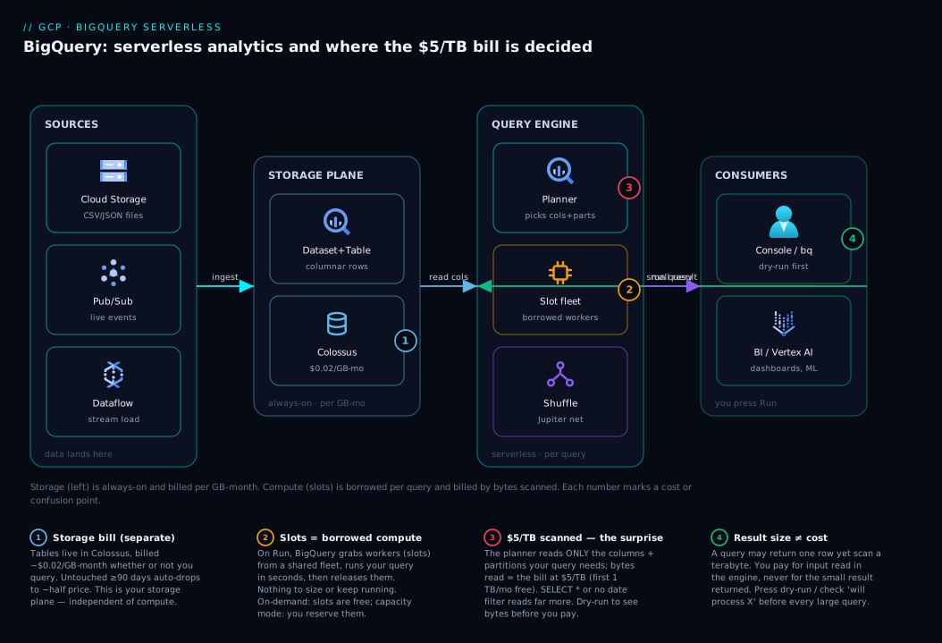
Let’s tie the pieces together visually. The diagram below traces a single query from the moment data arrives to the moment you read an answer — and it marks, with numbered badges, the four cost-and-confusion points every beginner needs to internalise.
Reading left to right: data enters from sources — files dropped in Cloud Storage, or live events flowing through Pub/Sub and a streaming pipeline like Dataflow — and lands in BigQuery as rows in a table inside a dataset. That table physically lives in Colossus storage (badge 1: this is your storage bill, separate and always-on, $0.02/GB/month active). When you press Run from a tool — the Console, the bq CLI, a BI dashboard, or even Vertex AI for ML — the query engine (badge 2) borrows slots from Google’s shared fleet, and those workers read only the columns and partitions your query needs from storage over the Jupiter network. The amount they read is your compute bill: in on-demand mode, $5 per TB scanned (badge 3). Workers shuffle and aggregate, then the small result returns to you (badge 4) — and you were charged for what was read, never for what was returned. The whole round trip is seconds, and the worker fleet vanishes the instant it’s done.
The two halves to keep separate in your head are the storage plane (left — durable, always there, billed per GB-month) and the compute plane (the borrowed slots — ephemeral, billed per query by bytes scanned). That separation is the entire architecture.
Real-world scenario
Company: Tindlo, a 14-person direct-to-consumer coffee subscription startup based in Bengaluru. The workload: every page view, add-to-cart, checkout and email open across their site and app streams in real time, landing in a single BigQuery table, analytics.events. By month four they had 2.1 billion rows / 1.4 TB in that table, growing ~12 GB/day. Two analysts and a founder ran dashboards and ad-hoc queries against it all day.
What went wrong. Tindlo’s founder, comfortable with SQL but new to BigQuery, built every dashboard tile and every exploratory query the way he’d learned on a small Postgres database: SELECT * FROM events WHERE ..., often without a date filter because “I might want to compare to last month.” The table had no partitioning — it was one flat 1.4 TB blob. A single dashboard with eight tiles, refreshing every 15 minutes, was running eight SELECT * scans of the full table, four times an hour, twelve hours a day. Each full scan was ~1.4 TB ≈ $7. Do the math: 8 tiles × 4/hr × 12 hr × 30 days × $7 ≈ $80,640/month of compute — for one dashboard. The first month’s bill (mercifully caught on day 9 by a billing alert) was already past ₹4 lakh and climbing.
The diagnosis. A 20-minute look at the INFORMATION_SCHEMA.JOBS view — which logs total_bytes_processed for every query — made it instantly obvious: 96% of all bytes scanned came from SELECT * queries with no date filter on the un-partitioned table. The dry-run estimate on a single dashboard tile read “will process 1.4 TB” — a number nobody had ever looked at.
The fix, in three moves. First, they re-created the table partitioned by event_date and clustered by country, event_type. Second, they rewrote every query to name only the columns it used (typically 4–6 of 47) and to always include a WHERE event_date BETWEEN ... filter. Third, they set a per-day billing cap of 2 TB on the project so no future mistake could exceed ~$10/day. The dashboard tile that had scanned 1.4 TB now scanned ~6 GB (one day, six columns) — a 230× reduction. The same eight-tile dashboard dropped from ~$80k/month to under $150/month. Storage stayed flat at ~$28/month. Total bill: ₹19,000/month instead of a runaway six-figure disaster — with zero loss of functionality.
The lesson, and the reason this scenario is here: BigQuery never refused the expensive query or warned them — it obediently scanned 1.4 TB every time it was asked. The guardrail was never going to come from the platform. It came from understanding the cost model and adding two things: a partition filter and a billing cap.
Advantages and disadvantages
BigQuery is the right default for analytics on Google Cloud, but it isn’t universally the right tool. Here’s the honest trade-off.
| Advantages | Disadvantages |
|---|---|
| Zero infrastructure — nothing to provision, patch, or scale | No visible cost ceiling by default; careless queries spend real money |
| Scales to petabytes; big queries finish in seconds | Not for transactional / OLTP workloads (no fast single-row updates) |
| Storage and compute billed separately and independently | The cost model is unintuitive until learned (the whole point of this article) |
| Pay only for queries you run (on-demand) | Per-query latency is seconds, not milliseconds — wrong for app back-ends |
| Standard SQL — no new query language to learn | Streaming inserts and some features carry separate charges |
| Free 1 TB scan + 10 GB storage every month | High steady volume can be cheaper on a competitor or on slots — must model it |
| Built-in ML (BigQuery ML), geospatial, and federated queries | Cross-region queries and egress can add cost and complexity |
| Automatic replication and durability | Deleting/altering huge tables and DML have their own cost considerations |
When each side matters: the advantages dominate for the overwhelmingly common case — a team that needs to analyse large, append-mostly datasets (logs, events, transactions-after-the-fact, IoT telemetry) with SQL and dashboards, without hiring a data-platform team. The disadvantages bite in two situations. First, if you mistake BigQuery for an application database and try to serve per-user reads at millisecond latency — use Cloud SQL or Firestore for that, and let BigQuery handle the analytics behind it. Second, if you run BigQuery on-demand without ever learning the cost model — then “pay only for what you query” becomes “pay for every careless SELECT *,” and the lack of a default ceiling turns from a feature into a footgun. Both disadvantages are avoidable; neither is a reason to avoid BigQuery, just reasons to use it knowingly.
Hands-on lab
Let’s make it real. This lab is free-tier-friendly: it uses tiny data and one of Google’s free public datasets, so your scans stay well under the 1 TB/month free allowance. You’ll create a dataset, load a small table, partition it, run a dry run, run a real query, set a cost guardrail, and tear it all down. Everything runs in Cloud Shell — no local install.
Step 0 — Set your project.
gcloud config set project YOUR_PROJECT_ID
PROJECT=$(gcloud config get-value project)
Step 1 — Create a dataset (a folder for tables), pinned to a region.
bq --location=US mk --dataset \
  --description "BigQuery beginners lab" \
  "${PROJECT}:bqlab"
# Dataset 'YOUR_PROJECT:bqlab' successfully created.
Step 2 — Practise the cost model on a public dataset without spending. Google hosts free public datasets you can query (you pay only for your scan bytes, and this stays in free tier). Dry-run a query first — always.
# Dry run: how much WOULD this scan? (no charge, no run)
bq query --use_legacy_sql=false --dry_run \
'SELECT name, SUM(number) AS births
 FROM `bigquery-public-data.usa_names.usa_1910_2013`
 WHERE state = "CA" AND year = 2000
 GROUP BY name ORDER BY births DESC LIMIT 10'
# -> running this query will process ~7 MB of data.  (~$0.00003)
Now compare what SELECT * would have cost on the same table:
bq query --use_legacy_sql=false --dry_run \
'SELECT * FROM `bigquery-public-data.usa_names.usa_1910_2013`'
# -> will process a much larger number — see the difference columns make
Step 3 — Run the cheap query for real and see the answer.
bq query --use_legacy_sql=false \
'SELECT name, SUM(number) AS births
 FROM `bigquery-public-data.usa_names.usa_1910_2013`
 WHERE state = "CA" AND year = 2000
 GROUP BY name ORDER BY births DESC LIMIT 10'
Expected output (truncated):
+----------+--------+
|   name   | births |
+----------+--------+
| Daniel   |  ...   |
| Anthony  |  ...   |
| ...      |  ...   |
+----------+--------+
Step 4 — Create a partitioned table of your own and watch the cost lever work. We’ll build a date-partitioned table from a public weather-style example using a query:
bq query --use_legacy_sql=false \
--destination_table "${PROJECT}:bqlab.names_by_year" \
--time_partitioning_field report_date \
--time_partitioning_type DAY \
--replace \
'SELECT name, state, number,
        DATE(year, 1, 1) AS report_date
 FROM `bigquery-public-data.usa_names.usa_1910_2013`
 WHERE year BETWEEN 2000 AND 2003'
Step 5 — Prove the partition saves bytes. Dry-run a query that filters to one partition vs one that doesn’t:
# Filtered to one partition: scans only that slice
bq query --use_legacy_sql=false --dry_run \
'SELECT name, SUM(number) FROM `'"${PROJECT}"'.bqlab.names_by_year`
 WHERE report_date = "2001-01-01" GROUP BY name'
# vs. no filter: scans all partitions
bq query --use_legacy_sql=false --dry_run \
'SELECT name, SUM(number) FROM `'"${PROJECT}"'.bqlab.names_by_year`
 GROUP BY name'
The filtered version reports a fraction of the bytes — that’s partition pruning in action.
Step 6 — Set a guardrail: a per-query maximum bytes billed. This makes BigQuery refuse any query that would scan more than your limit, so a mistake can’t run up a bill:
# Cap any single query at 1 GB of scan; over that, it errors instead of running
bq query --use_legacy_sql=false --maximum_bytes_billed=1000000000 \
'SELECT * FROM `bigquery-public-data.usa_names.usa_1910_2013`'
# Error: Query exceeded limit for bytes billed: 1000000000. ...
That error is the system protecting you — exactly the seatbelt Tindlo wished they’d had on day one.
Step 7 — Tear down so you leave nothing behind.
bq rm -r -f --dataset "${PROJECT}:bqlab"
# removes the dataset and all tables in it
You’ve now exercised the entire cost model end to end: estimate before running, name only needed columns, partition to prune bytes, and cap the maximum a query can spend.
The same setup in Terraform
For anything beyond a throwaway lab, define your dataset and partitioned table as code so structure (and cost-saving partitioning) is never forgotten:
resource "google_bigquery_dataset" "analytics" {
  dataset_id                  = "analytics"
  location                    = "US"
  description                 = "Event analytics warehouse"
  default_table_expiration_ms = null  # keep tables; set ms to auto-expire

  # Least-privilege access: grant a group read, a service account write
  access {
    role          = "READER"
    group_by_email = "analysts@tindlo.example"
  }
  access {
    role          = "WRITER"
    user_by_email = "ingest-sa@my-project.iam.gserviceaccount.com"
  }
}

resource "google_bigquery_table" "events" {
  dataset_id = google_bigquery_dataset.analytics.dataset_id
  table_id   = "events"

  # Partition by day -> a WHERE event_date filter prunes scans (cost lever)
  time_partitioning {
    type                     = "DAY"
    field                    = "event_date"
    require_partition_filter = true  # FORCES a date filter -> no accidental full scans
  }

  # Cluster -> BigQuery skips blocks within a partition for these columns
  clustering = ["country", "event_type"]

  schema = jsonencode([
    { name = "event_date", type = "DATE",      mode = "REQUIRED" },
    { name = "user_id",    type = "STRING",    mode = "REQUIRED" },
    { name = "country",    type = "STRING",    mode = "NULLABLE" },
    { name = "event_type", type = "STRING",    mode = "NULLABLE" },
    { name = "payload",    type = "JSON",      mode = "NULLABLE" }
  ])
}
The single most valuable line there is require_partition_filter = true: it makes BigQuery reject any query that lacks a date filter, structurally preventing the exact full-table-scan mistake that nearly bankrupted Tindlo. Turning a best-practice into an enforced rule is how seniors design for cost safety.
Common mistakes & troubleshooting
These are the failure modes new BigQuery users actually hit, in roughly the order they hit them. Each is symptom → root cause → how to confirm → fix.
| # | Symptom | Root cause | How to confirm | Fix |
|---|---|---|---|---|
| 1 | Bill far higher than expected | SELECT * on wide tables |
INFORMATION_SCHEMA.JOBS → sort by total_bytes_processed; spot SELECT * |
Name only needed columns; never * on big tables |
| 2 | “Cheap” query scanned a TB | No partition filter on a large table | Dry-run shows huge bytes despite a WHERE |
Partition by date; filter on the partition column |
| 3 | LIMIT 10 still cost $5 |
LIMIT trims output, not input |
Dry-run the LIMIT query — bytes unchanged |
Use the free Preview tab to peek; filter to reduce scan |
| 4 | Same dashboard re-scans constantly | No result caching / volatile query | Job shows cacheHit: false repeatedly |
Stabilise query text; rely on 24-hr result cache; materialise |
| 5 | “Query exceeded limit for bytes billed” | Hit a maximum_bytes_billed guardrail |
Error names the limit | Working as intended — narrow the query, or raise the cap deliberately |
| 6 | Dry run says huge but result is one row | Confusing result size with scan size | Compare totalBytesProcessed vs rows returned |
Accept that cost = input read; reduce columns/partitions |
| 7 | Partitioning “didn’t help” | Filtered on a non-partition column | Dry-run with vs without the date filter | Filter on the partition column specifically |
| 8 | WHERE country='IN' scans whole column |
Country isn’t partitioned or clustered | Bytes don’t drop with the filter | Add clustering on country; or partition appropriately |
| 9 | Streaming data costs more than expected | Streaming inserts billed separately from queries | Billing report line for streaming | Batch-load via load jobs (free) where latency allows |
| 10 | Cross-region query failed or cost more | Dataset and query/region mismatch | Error: dataset not in the region; or egress charge | Keep query, datasets, and storage in the same location |
| 11 | Costs spiked overnight, no one querying | A scheduled query / BI tool auto-refreshing | JOBS view filtered by user_email of the service acct |
Right-size schedule frequency; add partition filters |
| 12 | “Table not found” after creating it | Wrong project/dataset qualifier or region | bq ls PROJECT:DATASET |
Use fully-qualified project.dataset.table; match region |
Two diagnostic commands worth memorising. To find your most expensive queries (the single best cost-debugging move):
-- Top 20 costliest queries in the last 7 days, by data scanned
SELECT
  user_email,
  job_id,
  ROUND(total_bytes_processed / POW(2,40), 3) AS tb_scanned,
  ROUND(total_bytes_processed / POW(2,40) * 5, 2) AS est_usd,
  query
FROM `region-us`.INFORMATION_SCHEMA.JOBS
WHERE creation_time > TIMESTAMP_SUB(CURRENT_TIMESTAMP(), INTERVAL 7 DAY)
  AND job_type = 'QUERY' AND state = 'DONE'
ORDER BY total_bytes_processed DESC
LIMIT 20;
And to confirm whether a query hit the free result cache (cached re-runs cost $0 and scan 0 bytes):
bq query --use_legacy_sql=false --format=prettyjson \
  'SELECT 1' 2>/dev/null | grep -i cacheHit
# A repeated identical query within 24h shows cacheHit: true -> free
Best practices
Crisp, production-grade rules — most of them are about seeing or limiting bytes.
- Never
SELECT *on a large or wide table. Name the columns you actually need. This single habit is the biggest cost lever you have. - Always dry-run an unfamiliar or large query before running it. Glance at “will process X” every single time. It’s free and it’s your seatbelt.
- Partition large tables by date (or the natural time column) and always filter on the partition column. Set
require_partition_filter = trueso a missing filter is rejected, not silently expensive. - Cluster tables on the columns you filter/group by most (
country,event_type,customer_id). Clustering lets BigQuery skip blocks within a partition. - Set a per-query
maximum_bytes_billedand a per-day project billing cap. A guardrail can’t be forgotten the way discipline can. - Lean on the free result cache. Identical queries within 24 hours return cached results for $0. Keep query text stable so it actually hits.
- Don’t use
LIMITfor cost control — it doesn’t reduce scan. Use the free Preview tab to eyeball data, and filters/partitions to reduce bytes. - Materialise expensive repeated work. If five dashboards all scan the same raw rows, compute a smaller summary table (or a materialised view) once and point them at it.
- Batch-load instead of streaming when latency allows. Load jobs are free; streaming inserts carry a separate per-row charge.
- Keep storage, datasets, and queries in the same region to avoid cross-region cost and complexity, and to satisfy data-residency needs.
- Watch
INFORMATION_SCHEMA.JOBSweekly to catch the top scanners early — that’s how Tindlo would have caught the problem on day one. - Model on-demand vs slots once you cross ~100 TB/month. Don’t assume; compute both from your real
JOBShistory.
Security notes
Even a beginner setup should get the basics right; BigQuery’s security is mostly IAM plus a couple of data-specific controls.
- Least-privilege IAM. Grant the narrowest role that works.
roles/bigquery.dataViewerlets someone read a dataset’s data;roles/bigquery.jobUserlets them run queries (and incur cost);roles/bigquery.dataEditorlets them write. Don’t hand outroles/bigquery.adminto analysts. The IAM model is the same members-roles-bindings system explained in Google Cloud IAM Explained Simply: Members, Roles, and Bindings (Without the Jargon). - Separate “can query” from “can pay.”
jobUseris what actually spends money (it runs jobs). Be deliberate about who has it, because in on-demand mode running a query is spending. - Use service accounts for pipelines, with least privilege. Ingestion should run as a dedicated service account with only
dataEditoron the target dataset — see GCP IAM and Service Accounts: Roles, Bindings and Least Privilege. - Column- and row-level security let you restrict which columns (e.g. PII) or which rows a viewer can see, without copying data into a second table — useful the moment a table mixes sensitive and non-sensitive fields.
- Encryption is automatic. Data is encrypted at rest and in transit by default; for stricter control you can supply your own keys (CMEK) via Cloud KMS.
- Datasets carry the access boundary. Permissions are granted at the dataset (and optionally table) level, so organise sensitive data into its own dataset rather than mixing it into a shared one.
- Authorized views let you expose a filtered slice of a table to a group that can’t see the underlying table — the standard pattern for sharing “just these columns/rows” safely.
Cost & sizing
What actually drives a BigQuery bill, and the rough numbers to anchor on (USD list price; ₹ at ~₹83/$, varies).
| Cost driver | How it’s priced | Rough figure | Lever to reduce |
|---|---|---|---|
| On-demand queries | $5 per TB scanned | $5/TB; first 1 TB/mo free | Fewer columns, partition filters |
| Active storage | Per GB-month, tables touched <90 days | ~$0.02/GB-mo (~$20/TB-mo) | Expire/delete unused tables |
| Long-term storage | Tables untouched ≥90 days | ~$0.01/GB-mo — auto-halved | Nothing — it’s automatic savings |
| Streaming inserts | Per GB ingested via streaming | ~$0.01–0.05/GB (region-varying) | Batch-load (free) when you can |
| Capacity / slots | Per slot-hour | ~$0.04/slot-hr (Standard) | Commit 1/3-yr for discount |
| Free tier | Monthly allowance | 1 TB scan + 10 GB storage | Stay within it for small workloads |
| Storage API / egress | Reads via Storage Read API, cross-region | Varies | Keep everything one region |
Sizing intuition for a small team: if your warehouse is a low-single-digit TB and your queries are well-scoped (named columns, date filters), expect an all-in bill of tens of dollars a month, often under $100 (₹8,000). The free tier alone (1 TB scan + 10 GB storage/month) covers genuinely small projects at $0. The bill only becomes scary when (a) someone SELECT *s a large table repeatedly, or (b) you’re at genuine scale (hundreds of TB scanned/month), at which point you should be on capacity pricing anyway. Set a daily billing cap from day one — in on-demand it’s the difference between a bad query costing $10 and costing $10,000.
A quick self-check on whether you’re sized/priced right:
| If… | Then you’re probably… | Action |
|---|---|---|
| Bill is a few $/month, queries scoped | Fine on free tier / on-demand | Just keep dry-running |
| Bill is tens–low hundreds $, spiky | Right on on-demand | Add caps; tidy SELECTs |
| Bill is hundreds $, steady, many queries | A candidate for slots | Model capacity vs on-demand from JOBS |
| One query/dashboard dominates the bill | Missing a partition filter or SELECT * |
Fix that one thing first — biggest win |
| Storage > query cost and growing | Hoarding cold tables | Set table expiry; let long-term pricing help |
Interview & exam questions
Useful for the Google Cloud Digital Leader and Associate Cloud Engineer exams, and for any data interview.
-
What does “serverless” mean for BigQuery, specifically? You don’t provision, size, patch, or scale any compute; Google runs a shared fleet and allocates capacity per query. You pay for query execution (bytes scanned, on-demand) or reserved slots, not for machines you keep running.
-
How is on-demand BigQuery priced? $5 per terabyte of data scanned (read) by a query, with the first 1 TB per month free. It’s based on input bytes read, not rows returned, query time, or result size.
-
Why can
SELECT *be so much more expensive than naming columns? BigQuery uses columnar storage, so a query reads only the columns it references.SELECT *reads all columns, scanning far more bytes — often 10–50× more on a wide table — and you pay per byte scanned. -
Does
LIMIT 10reduce query cost in on-demand mode? No.LIMITreduces the result returned, not the data scanned; BigQuery still reads the full columns to find rows. Use partition/column reduction to cut cost, or the free Preview tab to peek. -
How do you estimate a query’s cost before running it? Run a dry run (
--dry_runin the CLI, or read the “will process X” estimate in the Console). It reports bytes that would be scanned, free and without executing. -
When should you choose capacity (slots) over on-demand? When you run a high, steady volume of queries — roughly hundreds of TB scanned per month — so a flat slot rate beats per-byte pricing, or when you need a predictable cost ceiling. Below that, on-demand is simpler and usually cheaper.
-
How does partitioning reduce cost? Partitioning splits a table (usually by date) into slices; a query filtering on the partition column reads only the matching slices (“partition pruning”), scanning far fewer bytes.
require_partition_filterenforces that a filter is present. -
Partitioning vs clustering — what’s the difference? Partitioning physically separates data into slices (typically by date) you can prune with a filter. Clustering sorts rows within each partition by chosen columns so BigQuery can skip irrelevant blocks. They stack: partition by date, cluster by the columns you filter/group on.
-
What’s the difference between active and long-term storage? A table (or partition) not modified for 90 consecutive days automatically drops to long-term storage at roughly half the active price. It’s automatic and requires no action; querying it doesn’t change the price, only modifying it resets the clock.
-
How do you prevent a runaway BigQuery bill? Set
maximum_bytes_billedper query, a per-day project billing cap,require_partition_filteron big tables, and least-privilege IAM (limit who hasjobUser). MonitorINFORMATION_SCHEMA.JOBSfor top scanners. -
Is BigQuery a good choice for an application’s transactional database? No. BigQuery is for analytics over large datasets, with second-scale latency and no fast single-row updates. Use Cloud SQL or Firestore for transactional/OLTP workloads and stream the data into BigQuery for analysis.
-
What does the result cache do for cost? An identical query re-run within 24 hours returns the cached result for $0 and scans 0 bytes. Keeping query text stable (e.g. in dashboards) lets it hit the cache and avoid re-scanning.
Quick check
- In on-demand mode, what exactly are you billed for — rows returned, query time, or bytes scanned?
- Why does
SELECT user_idcost far less thanSELECT *on the same table? - True or false: adding
LIMIT 100to a query reduces its on-demand cost. - What command lets you see a query’s cost before running it, for free?
- You scan ~250 GB in a query (and you’ve already used your free TB this month). Roughly what does it cost?
Answers
- Bytes scanned (data read from storage). Not rows returned, not time, not result size.
- Because BigQuery stores data by column (columnar).
SELECT user_idreads only that one column’s bytes;SELECT *reads all columns, scanning far more. - False.
LIMITtrims the result, not the data scanned — the full columns are still read, so cost is unchanged. - A dry run —
bq query --dry_run ...on the CLI, or the “will process X GB” estimate shown in the Console. It reports bytes without running or charging. - About $1.22: 250 GB ÷ 1024 ≈ 0.244 TB × $5 ≈ $1.22.
Glossary
- BigQuery — Google Cloud’s serverless data warehouse for analysing very large datasets with SQL.
- Serverless — A model where you don’t provision or manage machines; you pay for the work (queries) you run, and the provider runs the infrastructure.
- Dataset — A region-pinned container that holds tables and views; the unit at which access is commonly granted.
- Table — Your data organised in rows and columns; the object you query.
- Columnar storage — Storing all values of a column together (rather than all values of a row), so a query reads only the columns it needs.
- Bytes scanned — The amount of data a query physically reads from storage; the basis of on-demand billing.
- On-demand pricing — Paying $5 per terabyte of data scanned (first 1 TB/month free); the default model, with no commitment.
- Slot — BigQuery’s unit of compute capacity (a share of a worker); what you reserve under capacity pricing.
- Capacity pricing (slots / Editions) — Paying for a quantity of slots over time and running queries within that capacity, instead of per-byte.
- Dry run — A validation that reports how many bytes a query would scan, without executing it or charging you.
- Partition — A slice of a table (commonly by date); filtering on the partition column lets BigQuery skip non-matching slices (“pruning”).
- Clustering — Sorting rows within partitions by chosen columns so BigQuery can skip irrelevant data blocks.
- Result cache — A 24-hour cache that returns an identical query’s prior result for $0, scanning 0 bytes.
- Active vs long-term storage — Tables modified within 90 days (active) vs untouched ≥90 days (long-term, ~half price, automatic).
- Colossus — Google’s distributed storage system where BigQuery tables physically live, separate from compute.
- INFORMATION_SCHEMA.JOBS — A built-in view logging every query’s metadata, including bytes processed — your cost-debugging source of truth.
Next steps
- Go deeper on the mechanics — datasets, tables, partitioning internals, slots and the full pricing surface — in Google BigQuery, In Depth: Datasets, Tables, Partitioning, Slots & Pricing.
- Master the optimisation craft (partitioning, clustering, reservations, query rewriting) in Taming BigQuery Cost and Performance: Partitioning, Clustering, and Reservations.
- See where the data comes from in an event pipeline that feeds BigQuery: GCP Pub/Sub and Event-Driven Architecture: Decouple and Scale.
- Understand the cheap storage layer that often sits in front of BigQuery for raw files: Google Cloud Storage Classes and Lifecycle: Cost-Optimized Data.
- Lock down who can query and who can pay with Google Cloud IAM Explained Simply: Members, Roles, and Bindings (Without the Jargon).